Computer Systems Science & Engineering DOI:10.32604/csse.2022.019799
Article

Convolutional Neural Network Auto Encoder Channel Estimation Algorithm in MIMO-OFDM System

I. Kalphana1,* and T. Kesavamurthy2

1Government College of Engineering, Salem, 636011, India
2PSG College of Technology, Coimbatore, India
*Corresponding Author: I. Kalphana. Email: kalphana@gcesalem.edu.in
Received: 26 April 2021; Accepted: 18 June 2021

Abstract: Higher transmission rate is one of the technological features of prominently used wireless communication namely Multiple Input Multiple Output-Orthogonal Frequency Division Multiplexing (MIMO–OFDM). One among an effective solution for channel estimation in wireless communication system, specifically in different environments is Deep Learning (DL) method. This research greatly utilizes channel estimator on the basis of Convolutional Neural Network Auto Encoder (CNNAE) classifier for MIMO-OFDM systems. A CNNAE classifier is one among Deep Learning (DL) algorithm, in which video signal is fed as input by allotting significant learnable weights and biases in various aspects/objects for video signal and capable of differentiating from one another. Improved performances are achieved by using CNNAE based channel estimation, in which extension is done for channel selection as well as achieve enhanced performances numerically, when compared with conventional estimators in quite a lot of scenarios. Considering reduction in number of parameters involved and re-usability of weights, CNNAE based channel estimation is quite suitable and properly fits to the video signal. CNNAE classifier weights updation are done with minimized Signal to Noise Ratio (SNR), Bit Error Rate (BER) and Mean Square Error (MSE).

Keywords: Deep learning; channel estimation; multiple input multiple output; least square; linear minimum mean square error and orthogonal frequency division multiplexing

1  Introduction

MIMO integrated with OFDM technique is one among the eminent broadband wireless access system comprising of peculiar features such as, huge system capacity and higher data rates deprived of additional bandwidth and power consumption [1]. Channel estimation in a precise manner is highly necessitated for obtaining the transmitted signal through channel equalization. Also, it requires precise Channel State Information (CSI) of the system’s receiver end for transmitting signal coherent detection, which is regarded as significant challenge for achieving optimum performance of MIMO-OFDM systems. While comparing coherent detection with non-coherent detection technique considering 3 to 4 dB loss in SNR. This huge loss can be mitigated by developing channel estimation techniques for providing CSI at the receiver, for transmitting information from coherent detection in wireless communication systems. The most important issue to be resolved is the accurate Channel Estimation (CE) in wireless communications [2–5].

In digital communication systems, Adaptive Channel Estimation (ACE) process are performed [6,7], in which an adaptive filter is utilized for channel information estimation through linear channel estimation techniques [8]. Linear channel estimation techniques such as Least Squares (LS) algorithms are widely used because of its reduced computational complexity and simple to implement. Least Mean Square (LMS) algorithm is one among the commonly used ACE approaches with quite less computational complexity and also there is meager performance for Mean Square Error (MSE). The complexity can be reduced by utilizing simplified LMS algorithms like, Sign Data Normalized Least Mean Square (SDNLMS) algorithm [9].

Message transmission security to legitimate users is attained through deep learning-based secured communication [10]. Complex network in mobile communications such as Channel Estimation, Signal Detection, Modulation Recognition and Channel Equalization can be well handled through Deep Learning technology. Soltani et al. [11] utilized 2D image for presenting time-frequency channel fading matrix. A super-resolution network and a de-noising network might be deployed for achieving more precise channel estimation, in which pilot values are taken into account as a low-resolution image. Therefore, Super-Resolution (SR) network combined with a de-noising IR network is deployed for channel estimation. Balevi et al. [12] achieved one-bit quantization constraint by suggesting a deep neural network-based auto-encoder in OFDM receiver. A Convolutional Neural Network along with long short-term memory as the classifier is integrated in Modulation Recognition Algorithm [13] for modulation recognition robustness improvement.

Recently perfect free space optical communications are considered for developing a pilot independent Deep Learning-based channel estimator [14,15]. The suggested methodology offers satisfied performance to perfect channel estimation system which is validated by simulation outcome. These researches yield better performance for different task over current years. Hence it is concluded that Deep learning has grabbed the attention of various applications in communication systems. In addition to it, investigation for DNN structural properties were made considering depth and width owing to their modeling functions potent proficiency, i.e., DNNs expressiveness [16–18]. DNN expressive power increases exponentially with its depth for providing significant theoretical intuitions into DNNs greater performance practically. Hence it is substantiated that DL methods are specifically perfect for channel estimation but analytical interpretation of this phenomenon has to be concentrated yet.

Gao et al. [19] utilized Signal Processing Technique, which is done in block-by-block manner for dividing the receiver into signal detection and channel estimation subnet. Every subnet construction is done using DNN for initialization, which is a simple as well as conventional solution. When compared to Linear Minimum Mean Square Error technique by means of suggested model-driven DL receiver, precise channel estimation is attained and higher data recovery accuracy is highly achieved. When compared with prevailing approaches and Fully Connected Deep Neural Network (FC-DNN), Robustness in terms of signal-to-noise ratio is further validated through simulation outcomes, which is superior in terms of computational complexities or memory usage compared to FC-DNN approach.

Ye et al. [20] suggested a methodology in which, DNN model training was initially done by data generated on the basis of channel statistics, which was later utilized for online transmitted data recovering in direct way. DNN approach clearly explains the channel distortion and transmitted symbols which are detected with improved performance equivalent to Minimum Mean-Square Error (MMSE) estimator, validated through simulation outcome. DNN approach is more robust than traditional approaches, where smaller number of training pilots are used neglecting cyclic prefix and with existence of non-linear clipping noise. DNN are considered to be a capable tool even in complicated channel distortion and interference environment for estimating the channel and signal detection in wireless communications.

In this paper Convolutional Neural Network Auto Encoder (CNNAE) classifier interpretation is mainly concentrated for channel estimation in multiple-antenna systems. Also closed-form expression for CNNAE based channel estimation is formulated, which is considered to be highly sensitive for training data quality.

2  System Model and Channel Estimation

The system model for channel estimation is particularized by presenting conventional channel estimation methods and the CNNAE based method by multiple-antenna communication. LS and Linear Minimum Mean-Square Error (LMMSE) are deployed for estimation procedure. By using CNNAE technique through suggested channel estimation approach, the drawbacks of LS and LMMSE focused channel estimation strategies are mitigated.

2.1 System Model

Let multiple-antenna communication system with t0 antennas at Base Station (BS) and t1 at user side are assumed along with uplink channel in combination with block fading, comprising fixed channel fading. Uplink pilot is greatly utilized for channel estimation at BS in general procedure. Let τ represents transmitted pilot symbol with |τ|2 = 1. The representation of received symbol at BS is given by the subsequent t0 × t1 vector

x0=τh+n (1)

where h indicates t0 × t1 random channel vector amid BS and user. And n is t0 × t1 white noise vector with zero-mean and element-wise variance σn2 . The channel vector h is zero mean and with covariance matrix R = E{hhT}. E{.} represents expectation and tr{.} indicates matrix trace. The set cardinality is denoted by |.|. The notation || . ||2 signifies L2 norm, and diag{x} indicates a diagonal matrix with all elements in x at main diagonal. The notations (.)T, (.)* and (.)H denotes matrix transpose, conjugate and conjugate transpose respectively.

2.2 Conventional Channel Estimation

The extraction of h from x0 is the main objective of channel estimation which should be as precise as possible. The expert knowledge and signal model are the main basis for conventional estimation approaches.

2.2.1 LS Channel Estimator

From Eq. (1), LS estimate of h is initially derived by Eq. (2),

h^LS=1τx0=h+1τn (2)

and respective MSE is expressed by Eq. (3),

JLS=E{‖h−h^LS‖2} (3)

As shown in Eq. (3), the performance of the LS estimator is inversely proportional to the Signal-To-Noise Ratio (SNR) defined as 1/σ2 . Implementation is quite easier because no prior information of channel statistics is necessitated.

2.2.2 LMMSE Channel Estimator

LMMSE estimator utilizes signal model in Eq. (1) and channel statistics which is represented by ensuing Eq. (4),

h^LMMSE=R(R+σn2It0)−1x0 (4)

MSE computation of LMMSE estimator as in Eq. (5)

JLMMSE=tr{R(It0+1σn2R)}≤JLS (5)

This is merely smaller than that of LS estimator. The channels second order statistics is greatly utilized for further precise LMMSE channel estimation. Besides LMMSE estimator performances are sensitive to channel statistics imperfection, conversely there lies a challenge in acquiring this information practically. In contradiction to it, LS estimator is utilized in many scenarios as a result of its simplicity. Nonetheless its accuracy is comparatively small in contradiction with LMMSE estimator. In recent times CNNAE estimator has been developed as a capable substitute for addressing channel estimation in wireless communication systems. CNNAE estimator’s strong robustness and outstanding learning capacity helps it to be a potential tool for channel estimation in an imperfect and interference corrupted systems.

MIMO-OFDM system model designing is done followed by channel estimation using LS and LMMSE is performed which is given in ensuing sections. Also channel estimation is achieved by utilizing 16-QAM modulation [21]. 16-QAM modulation implementation has been carried out for different fading channels.

MIMO and OFDM integration is exploited in this research since it utilizes the benefits of both, like increase in wireless communication system capacity along with better-quality performances in multi path frequency-selective fading channels. Rayleigh fading is generally used for radio signal propagation effect evaluation such as amplitude fading. Non-Linear of Sight (NLOS) communication among transmitter and receiver is utilized in Rayleigh distribution based examination on multi path propagation background.

Subsequently the system used in Rayleigh fading is estimated using channel performance with consistent phases distributed over [0; 2π] Probability Density Function (PDF), which is represented in Eq. (6),

PR(r)=2rΩexp−r/Ω,r≥0, (6)

where ‘r’ represents a random variable with Rayleigh distribution ‘Ω’ and is identified by Eq. (7).

Ω=E(R2) (7)

Single parameter is utilized for Rayleigh distribution characterization. The earlier fading method fails for receiver with robust direct component of the signal.

Rician fading LOS path is presumed amid transmitter and receiver. It is suitable for multi path waves appearing at the receiver. The probability distribution function is specified by Eq. (8),

p(r)=rσ2exp⁡{−r2+A22σ2}J0(rAσ2),r≥0 (8)

where Jo ( ) is the 0th order modified Bessel function. It is described by Eq. (9),

J0(z)=∑n=0∞z2n22nn!n!,forz≫1 (9)

Next the Nakagami fading is the distributed gamma parametric fading, the data performance for obtaining approximate output was revealed by Eq. (10),

f(r)=2mmr2m−1ΩmΓ(m)exp⁡{−mr2Ω},m≥12:r≥0 (10)

where ‘m’ denotes Nakagami scale parameter which is fading parameter Ω and Г (m) are average power and gamma function.

3  Convolutional Neural Network Auto Encoder (CNNAE) Channel Estimation

In wireless communication systems, CNNAE estimator turns out to be a favorable substitute for addressing channel estimation. Especially for channel estimation in the inappropriate and interference corrupted systems, the CNNAE estimator can be considered as an effective model due to its robustness and efficient learning ability.

Assume that the CNNAE estimator P with an N-layer fully-connected Leaky Rectified Linear Unit (LReLU) CNN. x0∈χ⊆ℜt0 denotes the input of P; h∈H⊆ℜt0 indicates the output of P, in which χ and H signify input space and the output space. Consider f(x0, θ ) as the ℜt0→ℜt0 function that is denoted by P, in which all the parameters of P are indicated by θ and the estimated channel of the CNNAE estimator is notated by f(x0, θ ). Consider Z = χ×H as the sample space of training. A set of training samples drawn from the joint distribution of x0 and Zm={zi}i=1m={(x0,i,hi)}i=1m represents h, in which the number of training samples is signified by m. AE denotes the symmetrical CNN that is architecturally referred by three layers, namely input layer, hidden layer, and output layer, as depicted in Fig. 1. Subsequently the videos can be learned through this model in an unsupervised manner. AE tends to learn a latent or compressed representation of the input video, for which the reconstruction error within the input at the encoding layer and the respective reconstruction at the decoding layer is minimized.

Figure 1: Illustration of a single-layer CNNAE, neurons with cross denote the corrupted input neural units

In the encoding phase, an input vector x0∈χ⊆ℜt0 is processed, where a linear deterministic mapping and a nonlinear activation function l™ have been applied as given by Eq. (11),

αi=f(xi,θ)=l(W0,1x0,i+b0,1) (11)

in which a weight matrix with N layer is denoted by W0,1∈ℜNxt0 ; the encoding bias is represented by b0,1∈ℜt0 . A Leaky Rectified Linear Unit (LReLU) activation function is taken for signal x0. In the domain of deep learning, application of LReLU is proved to be significant as it provides optimal performance [22–24], as given in Eq. (12),

y={x0if x0,i≥0ωx0if x0,i≤0 (12)

The slope ω of the LReLU is fixed as 0.01 [25]. Subsequently a vector is decoded by applying further linear decoding matrix in Eq. (13),

hi=(W0,2αi+b0,2) (13)

Here, a decoding weight matrix is denoted by W0,2∈ℜt0xN and a bias vector is represented by b0,2∈ℜt0 . The reconstruction error of the cost function in Eq. (14) is reduced to learn signal extractors. In the cost function, the first term signifies the error term whereas the second term indicates a regularization term/weight decay term.

L(x0,h)=12∑i=1m‖x0,i−h0,i‖2+λ2‖W0,t‖2 (14)

The training video signal is signified by x0,i and reconstructed noise that removed video signal is denoted by h0,i. For constraining the anticipated activation of hidden nodes, the method [26] is presented due to the sparseness of hidden units. By adding the Regularization term, the hidden unit values are penalized, through which solely some of them get bigger than parameter ρ. Consequently many values of hidden units get lower than ρ. By denoting the sparse penalty term as KL(ρ||ρ^) it can be formulated by Eq. (15),

KL(ρ||ρ^)=ρlog⁡ρρ^+(1−ρ)log⁡1−ρ1−ρ^ (15)

Here, Kullback–Leibler divergence is represented by KL(·). The activation of hidden units in auto-encoder is notated by α which is discussed in Eq. (16),

ρ^=(1/m)∑i=1m[α(i)] (16)

As the average activation of α that is average on the training set xt0×N , then the objective function in the sparse auto encoder learning can be notated by Eq. (17),

Loss=L(x0,h)+β∑j=1NKL(ρ||ρ^) (17)

A large average activation of α is penalized over the training samples by assigning ρ small, for which the KL divergence is introduced i.e., weighed by a sparsity penalty parameter β in the objective function. Consequently activation of many hidden units has been driven by this penalization to be equal or near to zero, which leads to sparse connections within layers. Solely two states are involved in the neurons in P, i.e., with zero output or replicating input. Although the CNNAE based channel estimation proves to be efficient from theoretical point of view, it is being analyzed infrequently. CNNAE estimator learns a set of training data Zm that is brought from particular statistical framework. For measuring the variation of the estimated channel f(x0, θ ) and the true one h, the DL estimator requires a non-negative loss function ξ(f(x0,θ),hi) . The following Eq. (18) is formulated by adopting the square error as loss functions,

Jemp=1m∑Zi∈Zmξ(f(x0,θ),hi)=1m∑Zi∈Zm‖hi−f(x0,i,θ)‖22 (18)

The empirical loss is described by Eq. (19),

JCNNAE=EZ{ξ(f(x0,θ),h}=∑i=1υE{‖h−f(x0,θ)‖22|x0∈χi}ψ(χi) (19)

For the expected loss in which the probability ψ(χi) that x0 falls into χi . The parameters of P can be optimized by the CNNAE estimator by considering the CNNAE based channel estimation as a regression problem for which the empirical loss in Eq. (18) is minimized for, provided Zm and the channels from newly received signals are predicted through the optimized CNNAE estimator. Generally by applying the following statistical framework, the theoretical system in nonlinear communication systems is described by Eq. (20),

x0=fNL(τh+n) (20)

The nonlinear distortion imposed on the received signal is represented by fNL(.); conversely if fNL(.) is a linear function, the nonlinear model reduces to the linear model, Eq. (1) as expressed in Eq. (20). Consider Ai as the set of sample index that fall in to χi . Remember that (|A1|, … |Aυ|) is an i.i.d. multi nominal random variable with probability (ψ(χ1),…,ψ(χν)) and the constraint ∑i=1ν|Ai|=m . In the context of inaccurate training data, the calculation over the estimation MSE of the CNNAE estimator can be divided into two cases as described below,

Case 1: In this case, let her be the channel of inaccurate training data, then it distributes in a broader range than h and the associated statistical model of the training data can be expressed as the following Eqs. (21)–(22),

her=h+ϵ (21)

xer=τher+n (22)

Here, the t0 × t1 zero mean random error vector is represented by ϵ (which is independent of h) that includes covariance matrix Ωϵ=E{ϵϵT} .

Case 2: Assume that the training data’s input-output pair is produced from the statistical framework, as described in the Eqs. (23)–(24),

h=her+ϵ (23)

xer=τher+n (24)

Since x0 distributes in a broader range than xer , the probability that x0 locates at regions deprived of the necessity of training samples are higher than Case 1. If the discrepancy within h and her is large enough, the estimated channels of the CNNAE estimator related to the inputs at empty regions are completely arbitrary and undesirable. In such a scenario the CNNAE estimator lacks in providing a consistent estimate due to the difficulty of obtaining the estimation MSE in the form of analytic.

4  Results and Discussions

The entire implementation of the proposed channel estimation method in MIMO-OFDM with 8 × 8 has been carried out in MATLAB simulation and the performance has been measured based on the parameters, such as MSE, SNR, Symbol Error Rate (SER) and BER. During the analysis 16-QAM modulation is involved, where the phase offset zero is taken as the symbol order in binary. Since video signals have been exploited during the simulation of this work, they transfer an integer through the channels of Rayleigh, Rician and Nakagami by considering it as an input. Thus, the channel estimator implementation is determined by comparing the proposed and other LS and LMMSE methods, through that reduced MSE is ensured by the proposed method. Tab. 1 discuss about the details of simulation parameters used for evaluating the channel estimation methods.

4.1 Simulation Results

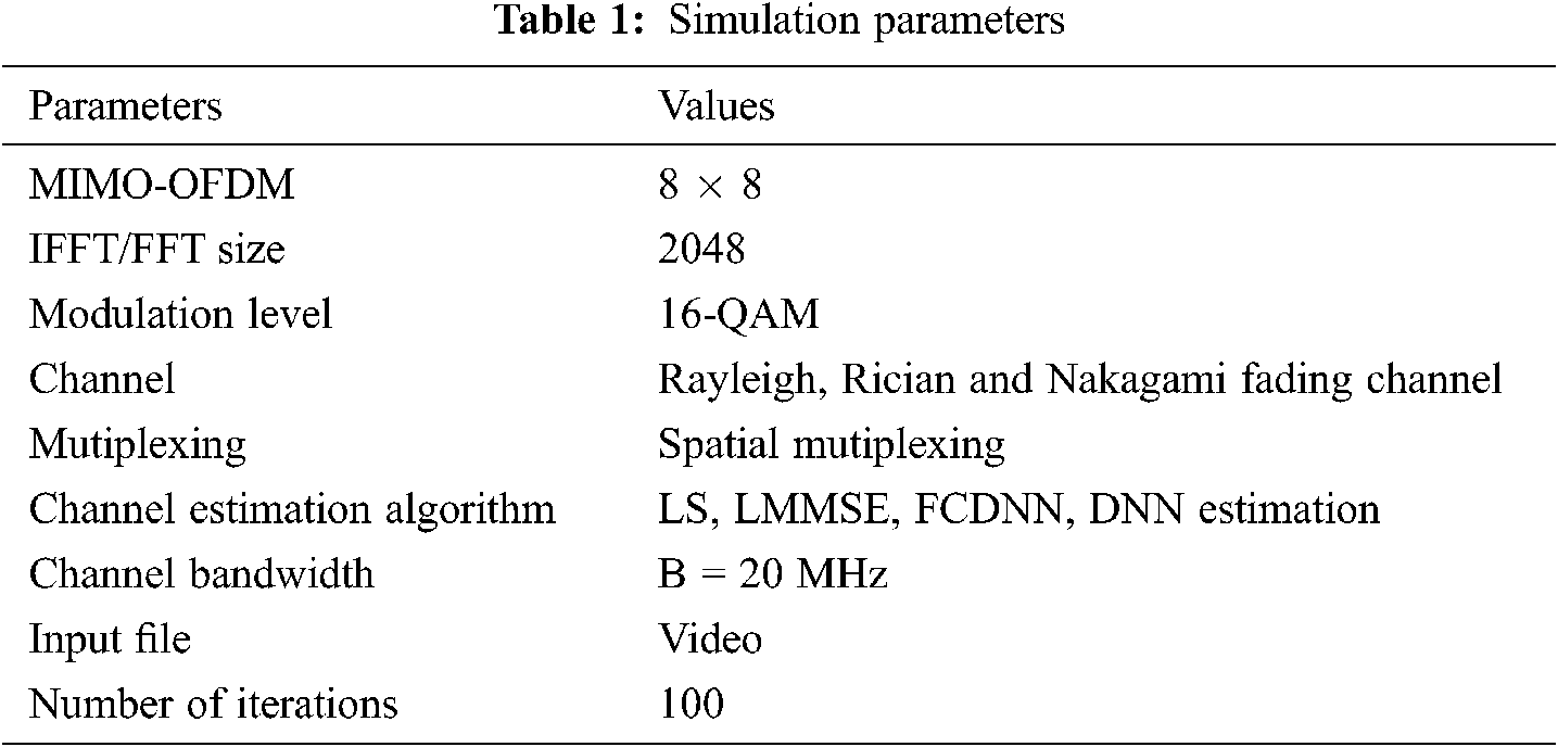
In this section the simulation outcomes of different channel estimation techniques have been depicted as three individual fading channels. With regard to error analysis, the channel estimation results have been measured using each of the metrics. The simulation outcomes of channel estimation approach for Rayleigh channel are presented numerically in Tab. 2, Nakagami channel are presented numerically in Tab. 3 and Rician channel are presented numerically in Tab. 4.

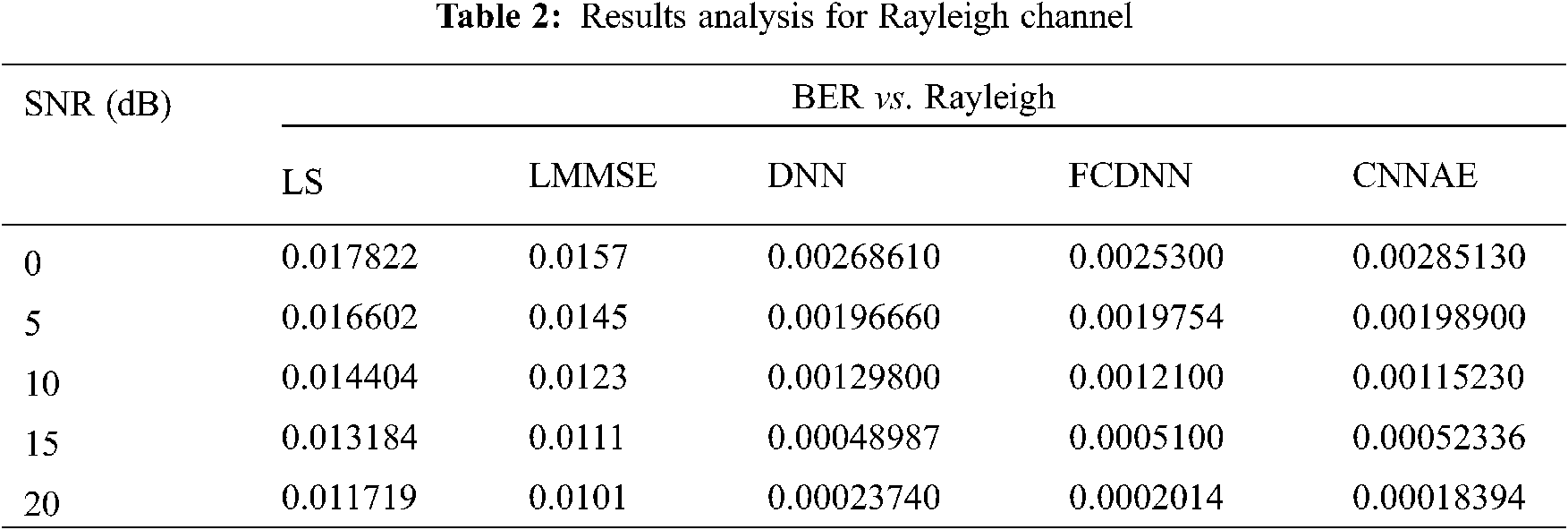
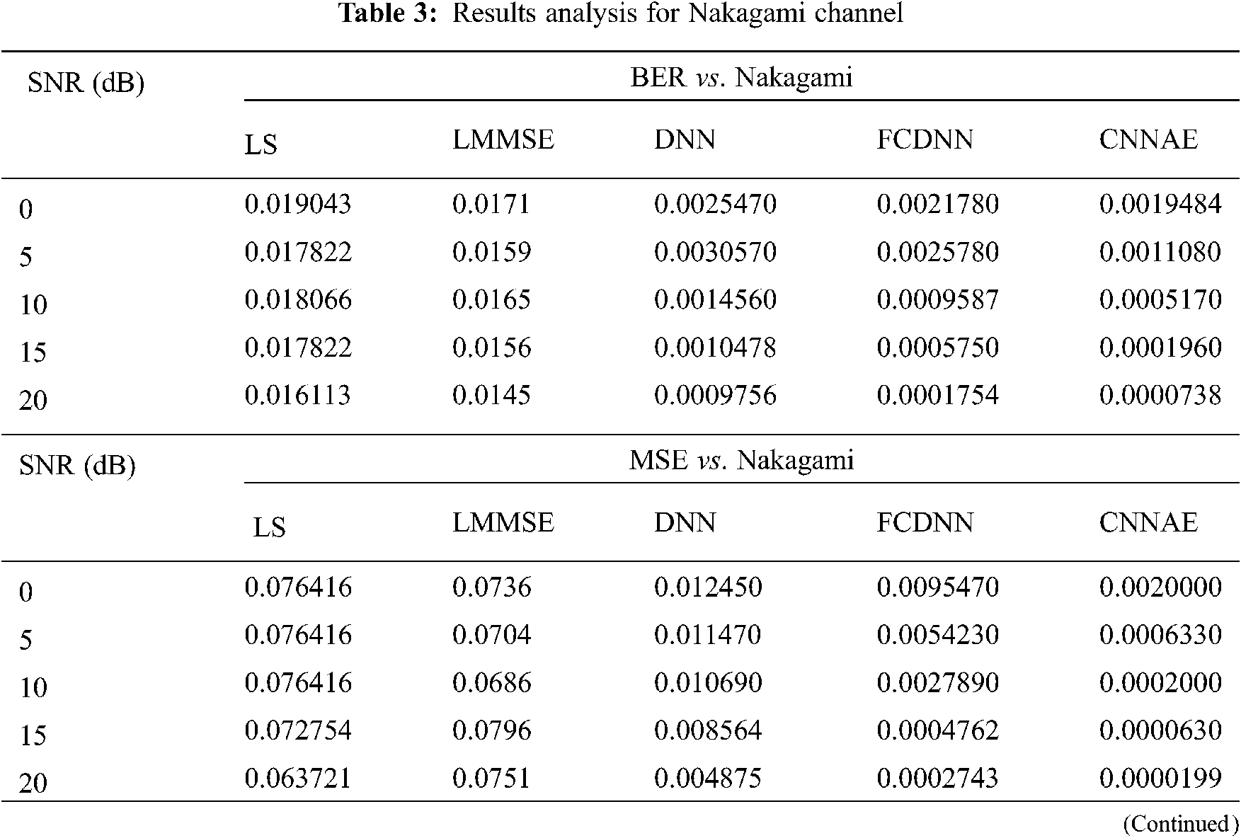
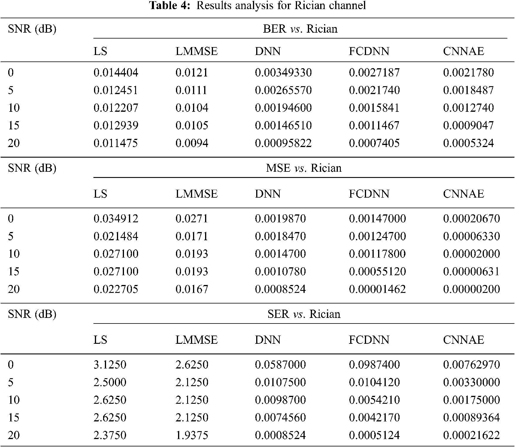
Figure 2: MSE vs. SNR using LS, LMMSE and proposed estimation for different fading environments (a) MSE vs. SNR for Rayleigh channel (b) MSE vs. SNR for Rician channel (c) MSE vs. SNR for Nakagami channel

In Fig. 2 MSE and SNR values have been compared for varied fading channels by applying the existing channel estimation methods like LS, LMMSE, DNN, FCDNN and proposed CNNAE method to evaluate their performance. The graphs demonstrate the efficiency of the proposed CNNAE approach to outperform the existing methods by providing the better result in each fading environment, as represented in Figs. 2a–2c. Besides the multiplication, SNR helps reducing the Mean Square Error. As depicted in Fig. 2c the CNNAE algorithm delivers the MSE of 0.0000199 for Nakagami Channel in SNR at 20 dB. Whereas, the existing LS, LMMSE, DNN and FCDNN approaches provide 0.063721, 0.0751, 0.004875, and 0.0002743, respectively, which are considerably in higher side of BER.

Figure 3: BER vs. SNR using LS, LMMSE and proposed estimation for different fading environments (a) BER vs. SNR for Rayleigh channel (b) BER vs. SNR for Rician channel (c) BER vs. SNR for Nakagami channel

In Fig. 3 in order to evaluate their performance BER and SNR values have been compared for different fading channels by utilizing the existing channel estimation methods like LS, LMMSE, DNN, FCDNN and proposed CNNAE method. The graphs depict the proficiency of the proposed CNNAE method to surpass the existing methods by providing the optimal result in each fading environment, as represented in Figs. 3a–3c. However, the augmentation of SNR helps to minimize the Bit Error Rate. As demonstrated by Fig. 3c, the proposed CNNAE provides the BER of 0.0000738 for Nakagami Channel in SNR at 20 dB. Whereas the existing LS, LMMSE, DNN and FCDNN approaches provide 0.016113, 0.0145, 0.0009756, and 0.0001754 respectively, this has the higher BER than the proposed system.

Figure 4: SER vs. SNR using LS, MMSE and proposed estimation for different fading environments (a) SER vs. SNR For Rayleigh channel (b) SER vs. SNR for Rician channel (c) SER vs. SNR for Nakagami channel

Fig. 4 Compares the SER and SNR values obtained for different fading channels by exploiting the existing channel estimation methods like LS, LMMSE, DNN, FCDNN, and proposed CNNAE method for evaluating their performance. The graphs depict that the proposed CNNAE method is capable of outperforming the existing methods by securing optimal result in each fading environment as represented in Figs. 4a–4c. As illustrated by Fig. 4c the proposed CNNAE provides the SER of 0.00021622 for Rician Channel in SNR at 20 dB. LS, LMMSE, DNN and FCDNN approaches has given higher SER of 2.3750, 1.9375, 0.0008524 and 0.0005124 respectively.

5  Conclusion and Future Work

In this study a Convolutional Neural Network Auto Encoder (CNNAE) based Channel Estimation Algorithm is introduced for MIMO-OFDM System, accompanied by appropriately selected inputs. The CNNAE is capable of utilizing the channel variation features from the previous channel estimates, through which it reduces the signal noises. The proposed CNNAE channel estimation algorithm is implemented to conventional estimations like LS and LMMSE for enhancing the channel estimation performance. Channel estimation is obtained on the basis of the property namely CNNAE with LReLU activation function, which is mathematically the same as the set of local linear functions. CNNAE channel estimation is presented for learning a latent or compressed representation of the input signals by which the reconstruction errors occurring within input at the encoding layers and corresponding reconstruction at the decoding layer has reduced considerably. Subsequently for fading channels such as Rician, Rayleigh and Nakagami, the CNNAE based channel estimation is carried out. The proposed method optimizes the derived channel model by executing the conventional approaches of channel estimation. During the experiments the implementation has been performed for 16-QAM, besides completely simulated using MATLAB simulator. Empirical findings depict that the significant capability of the proposed CNNAE based channel estimation approach, surpass the existing techniques as regards various fading models of MIMO-OFDM. By considering the parameters such as MSE, SNR, SER and BER, the performance of the proposed and prevailing methodologies are compared and evaluated. In future, this study can be extended through exploring the possible ways of executing the advanced and multifaceted stacking ensemble architectures like Recurrent Neural Network (RNN) and Convolutional Neural Networks (CNNs) in the channel estimation operation of wireless communications.

Funding Statement: The authors received no specific funding for this study.

Conflicts of Interest: The authors declare that they have no conflicts of interest to report regarding the present study.

This work is licensed under a Creative Commons Attribution 4.0 International License, which permits unrestricted use, distribution, and reproduction in any medium, provided the original work is properly cited.