Computer Systems Science & Engineering DOI:10.32604/csse.2022.020079
Article

Statistical Inference of Sine Inverse Rayleigh Distribution

Abdullah, Ali H. Ahmadini*

Department of Mathematics, Faculty of Science, Jazan University, Jazan, Saudi Arabia
*Corresponding Author: Abdullah Ali H. Ahmadini. Email: aahmadini@jazanu.edu.sa
Received: 07 May 2021; Accepted: 08 June 2021

Abstract: We study in this manuscript a new one-parameter model called sine inverse Rayleigh (SIR) model that is a new extension of the classical inverse Rayleigh model. The sine inverse Rayleigh model is aiming to provide more fitting for real data sets of purposes. The proposed extension is more flexible than the original inverse Rayleigh (IR) model and it hasmany applications in physics and medicine. The sine inverse Rayleigh distribution can havea uni-model and right skewed probability density function (PDF). The hazard rate function (HRF) of sine inverse Rayleigh distribution can be increasing and J-shaped. Several of thenew model’s fundamental characteristics, namely quantile function, moments, incompletemoments, Lorenz and Bonferroni Curves are studied. Four classical estimation methods forthe population parameters, namely least squares (LS), weighted least squares (WLS), maximum likelihood (ML), and percentile (PC) methods are discussed, and the performanceof the four estimators (namely LS, WLS, ML and PC estimators) are also compared bynumerical implementations. Finally, three sets of real data are utilized to compare the behavior of the four employed methods for finding an optimal estimation of the new distribution.

Keywords: Sine generated family; inverse Rayleigh distribution; classic estimation methods; applications

1  Introduction

Reference [1] investigated a significant distribution in analysis of lifetime, namely the inverse Rayleigh (IR) model. The IR model’s considered probability density function (PDF) and the corresponding distribution function (CDF) are given by

g(y)=2θy−3e−θy2,θ>0,y>0. (1)

and

G(y)=e−θy2,θ>0,y>0. (2)

Much effort has been invested in the literature on estimating the IR model; see, for instance, [2–10].

In last years, several extensions for the IR model were established by means of various generalization methods such as beta IR, transmuted IR (TIR), modified IR, transmuted modified IR, Kumaraswamy exponentiated IR, weighted IR and odd Fréchet IR and half logistic IR models as mentioned in [2–9].

In the last years, many different statisticians are attracted by generated families of distributions as: sine generated (S-G) by [10], Type II half logistic-G by [11], odd Frèchet-G by [12], truncated Cauchy power-G by [13], transmuted odd Fréchet-G by [14], exponentiated M-G by [15], Topp-Leone odd Fréchet-G studied in [16], among others.

For instance, for S-G the CDF and the PDF are

F(y;ξ)=sin[π2G(y;ξ)],x∈R.   (3)

and

f(y;ξ)=π2g(y;ξ)cos[π2G(y;ξ)],x∈R. (4)

where g(y;ξ) considers a PDF of baseline distribution.

Now, we put forward a novel lifetime model with one parameter named sine inverse Rayleigh (SIR) distribution, whose CDF with parameter θ is obtained by employing (2) in (3) as

F(y)=sin[π2e−θy2], y>0,  θ>0,  (5)

Likewise, by combining (1), (2) and (4), one obtains the corresponding PDF to (5) as

f(y)=πθ2y3e−θy2cos[π2e−θy2], y>0,  θ>0,   (6)

where θ is a scale parameter.

When the random variable Y has an SIR model, one can define X’s hazard rate function (HRF), reversed HRF, cumulative HRF, and survival function (SF) as

R(y)=1−sin[π2e−θy2] ,

h(y)=πθy3e−θy2cos[π2e−θy2] 1−sin[π2e−θy2], 

τ(y)=πθy3e−θy2cot[π2e−θy2], 

and

H(y)=−ln(1−sin[π2e−θy2]) .

Figs. 1 and 2 present the PDF and HRF plots of the SIR distribution, respectively, for various θ values.

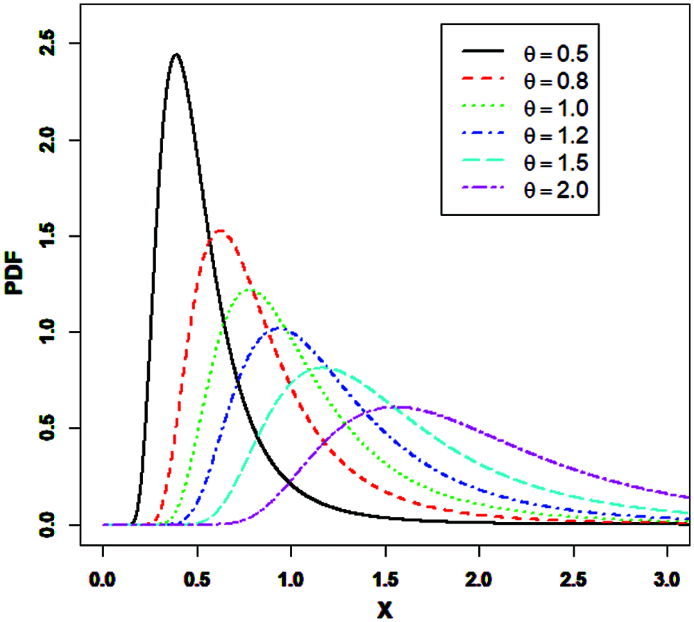
Figure 1: Plots of the PDF the SIR distribution

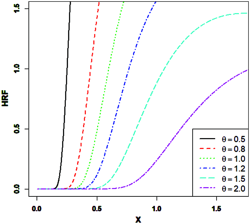
Figure 2: Plots of the HRF the SIR distribution

Figs. 1 and 2 exhibit that the SIR distribution can have a uni-model and right skewed PDF, while its HRF can be J-shaped and increasing.

The remaining parts of this manuscript are presented as follows. Section 2 introduces structural characteristics of SIR distribution including; quantile function, moments, incomplete moments, and Lorenz and Bonferroni curves. Section 3 discusses some estimators for SIR distribution parameters on the basis of four different methods of estimations of least squares (LS), weighted least squares (WLS), maximum likelihood (ML), and percentile (PC). Simulation schemes are performed in Section 4. Three sets of data for real-life applicationare utilized for comparing the behavior of the four methods of estimating the new distribution in Section 5. Several concluding remarks close the work.

2  Fundamental Properties

We study in this part several statistical characteristics of the SIR model.

2.1 Quantile Function

If Y~SIR then, the quantile function of SIR is

Q(u)=θ[ln(π2Arcsin(u))]−1.

and by taking u = 0.5 we get the median (M) as M=θ[ln(3)]−1.

2.2 Moments

Theorem 1: Assume that Y is an r.v. from SIR, thus the rth moment of SIR distribution is

μ´r=∑i=0∞θr2−1CΓ(1−r2)2(2i+1)1−r2,r2<1. (7)

Proof: Assume that Y is an r. v. with pdf (6). One can determine rth moments of SIR distribution from

μ´r=∫0∞⁡yrf(y)dy=πθ2∫0∞⁡yr−3e−θy2cos[π2e−θy2]dy,

By inserting the expansion cos[G(y)]=∑i=0∞⁡(−1)i(2i)![G(y)]2i,n to the previous equation then,

μ´r=∑i=0∞θ(−1)i(2i)!(π2)2i+1∫0∞⁡yr−3e−(2i+1)(θy2)dy,

The last equation can be rewritten as

μ´r=∑i=0∞⁡C∫0∞⁡yr−3e−(2i+1)(θy2)dy.

where C=∑i=0∞⁡θ(−1)i(2i)!(π2)2i+1.

Let Z=θy2 , then

μ´r=∑i=0∞⁡θr2−1C∫0∞⁡z−r2e−(2i+1)zdz.

Then,

μ´r=∑i=0∞θr2−1CΓ(1−r2)2(2i+1)1−r2.

The mgf of Y is

MX(t)=∑r=0∞trr!μ´r=∑r,i=0∞trθr2−1CΓ(1−r2)2r!(2i+1)1−r2.

obtain the incomplete moments, denoted by φs(t), of the SIR distribution as follows, where φs(t), defined by

φs(t)=∫0t⁡f(y;φ)dy. (8)

Using (8), φs(t) will be as given

φs(t)=∑i=0∞⁡C∫0t⁡ys−3e−(2i+1)(θy2)dy=∑i=0∞θs2−1CΓ(1−s2,(2i+1)(θt2))2(2i+1)1−s2, (9)

where Γ(s,t)=∫0tys−1e−ydy denotes the lower incomplete gamma function.

The Lorenz curve and the Bonferroni curve are generated, respectively, from following equations

LF(x)=φ1(y)E(Y)=∑i=0∞θ−12CΓ(12,(2i+1)(θt2))2(2i+1)12∑i=0∞θ−12CΓ(12)2(2i+1)12=∑i=0∞CΓ(12,(2i+1)(θt2))(2i+1)12∑i=0∞Cπ(2i+1)12,

and

BF(x)=LF(y)F(y;φ)=∑i=0∞CΓ(12,(2i+1)(θt2))(2i+1)12∑i=0∞Cπ(2i+1)12(sin[π2e−θy2] ).

The Zenga curves are given by

AF(y)=1−μ−(y)μ+(y)

where

μ−(x)=LF(y)

and

μ+(x)=∫t∞⁡f(y;φ)dy1−F(y).

3  Statistical Inference

The population parameters involved in the SIR model can be estimated by using four different methods of estimation namely; ML, LS, WLS and PC methods.

3.1 ML Estimators

To obtain the MLEs of the SIR model with a parameter θ, let Y1,…, Yn be observed values of this model. The log-likelihood function denoted by ℓ, can be expressed as

ℓ=nlogπ2+nlogθ−3∑i=1n⁡log(yi)−θ∑i=1n⁡(yi)−2+∑i=1n⁡log(cos[π2e−θ(yi)−2]).

The ML equation of the SIR model then becomes

∂ℓ∂θ=nθ−∑i=1n⁡(yi)−2+π2∑i=1n⁡(yi)−2e−θ(yi)−2tan[π2e−θ(yi)−2].

The MLEs of θ are then obtained by equating ∂ℓ/∂θ with zero and solving simultaneously these equations.

3.2 LS and WLS Estimators

Let Y1, Y2, …, Yn be an n-sized random sample (RS) from SIR model and denote the ordered samples in the RS by Y(1), Y(2), …, Y(n). The expectation and variance of this model do not depend the unknown parameter given by

E(F(Y(i)))=in+1,andvar(F(Y(i)))=i(n−i+1)(n+1)2(n+2),

In the above equations, F(Y(i)) represents the CDF of the model while Y(i) represents the ith order statistic (OS). Thus, the LSEs can be determined by obtaining the least sum of squared errors as follows,

∑i=1n[F(i)(y)−in+1]2,

regarding θ. Thus, the LSEs of the population parameter θ of SIR follow by calculating the minimum of the sum

∑i=1n⁡[sin[π2e−θ(y(i))2]−in+1]2,

regarding θ. Moreover, the LSEs of θ can be determined from

∑i=1n⁡[sin[π2e−θ(y(i))2]−in+1](1(y(i))2e−θ(y(i))2cos[π2e−θ(y(i))2])=0.

The WLSEs of θ can then be derived by calculating the minimum of the sum

∑i=1n(n+1)2(n+2)i(n−i+1)[sin[π2e−θ(y(i))2]−in+1]2,

regarding θ. Moreover, one can determine the WLSEs of θ from

∑i=1n(n+1)2(n+2)i(n−i+1)[sin[π2e−θ(y(i))2]−in+1](1(y(i))2e−θ(y(i))2cos[π2e−θ(y(i))2])=0.

3.3 PC Estimator (PCEs)

Let Y1,…,Yn denote an RS taken from SIR and assume that Y(1)< Y(2)<…<Y(n) is the corresponding OS. The PCEs of parameter θ are calculated by minimizing the next

∑i=1n⁡[ln(in+1)−ln(sin[π2e−θ(y(i))2])]2,

regarding θ.

4  Numerical Results

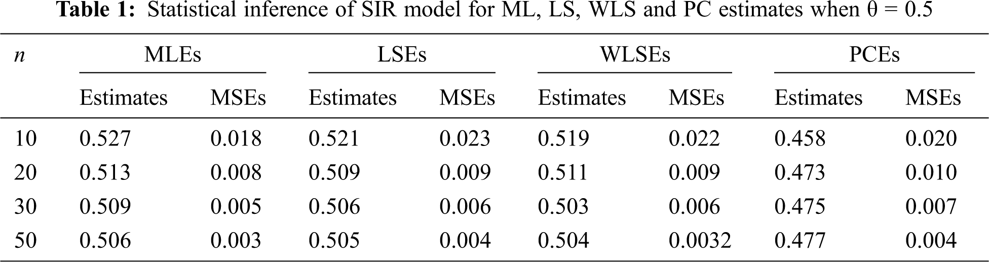
We generate 3000 RS Y1, …, Yn of sizes n = 10, 20, 30 and 50 from SIR were generated. Three different values of the parameter θ are chosen:

The parameter θ’s ML, LS, WLS and PC estimates are calculated. Subsequently, the MSEs of the estimate of the unknown parameter are determined. Numerical results are mentioned in Tabs. 1–3 and the following observations can be made.

•   The MSEs of ML estimates of θ are the lowest among all determined MSEs in almost every case.

•   The MSEs of all the estimates decrease with increasing sample sizes.

5  Applications to Real Data

Further we employ three real data sets for assessing the goodness-of-fit of the SIR model with the purpose of comparing the performance of the considered estimation methods.

We consider criteria including maximum likelihood (denoted by − ℓ^ ,) (B1), the Akaike information criterion (AIC) (B2), the consistent AIC (B3), the Schwarz criterion (B4) and the Hannan-Quinn information criterion (B5). The model that has lowest B1-B5 values is deemed the best one with respect to fitting the real data.

The first data set: contains the survival time (days) of 72guinea pigs with virulent tubercle bacilli infection, originally presented in [17].

The second data set: consists the waiting time (minutes) of 100 bank customers before they were served, as presented in [18].

The third data set: contains 100 results on the breaking stress (Gba) of carbon fibers, as presented in [19].

The parameters of SIR are estimated by the four estimation methods, namely the ML, LS, WLS and PC estimation methods. The efficiency of the estimation methods is the same in the three data sets as shown in Tabs. 4–6. We see that among the estimation methods adopted, ML provides the best results for the included data sets.

6  Conclusion

We study a new model called SIR. Some fundamental characteristics of the model are investigated. We estimate the model parameters according to the ML, LS, WLS and PC methods. Numerical experiments are carried out in order to comparatively explore the performance of the four different estimation methods. Numerical results show that ML performs better than LS, WLS and PC in almost all considered situations. Applications on three sets of real data indicate that the the ML method is superior in terms of the fits to the LS, WLS and PC methods.

Acknowledgement: The author is grateful to the academic editor and all four reviewers for their valuable comments that have contributed to significantly improve the quality on the article. I would like to thank TopEdit (https://www.topeditsci.com) for English language editing of this manuscript.

Funding Statement: The author received no specific funding for this study.

Conflicts of Interest: The author declare no conflict of interest.

This work is licensed under a Creative Commons Attribution 4.0 International License, which permits unrestricted use, distribution, and reproduction in any medium, provided the original work is properly cited.