Computer Systems Science & Engineering DOI:10.32604/csse.2022.020367
Article

Gaussian Kernel Based SVR Model for Short-Term Photovoltaic MPP Power Prediction

Yasemin Onal*

Department of Electrical and Electronics Engineering, Bilecik Seyh Edebali University, Bilecik, 11000, Turkey
*Corresponding Author: Yasemin Onal. Email: yasemin.onal@bilecik.edu.tr
Received: 20 May 2021; Accepted: 21 June 2021

Abstract: Predicting the power obtained at the output of the photovoltaic (PV) system is fundamental for the optimum use of the PV system. However, it varies at different times of the day depending on intermittent and nonlinear environmental conditions including solar irradiation, temperature and the wind speed, Short-term power prediction is vital in PV systems to reconcile generation and demand in terms of the cost and capacity of the reserve. In this study, a Gaussian kernel based Support Vector Regression (SVR) prediction model using multiple input variables is proposed for estimating the maximum power obtained from using perturb observation method in the different irradiation and the different temperatures for a short-term in the DC-DC boost converter at the PV system. The performance of the kernel-based prediction model depends on the availability of a suitable kernel function that matches the learning objective, since an unsuitable kernel function or hyper parameter tuning results in significantly poor performance. In this study for the first time in the literature both maximum power is obtained at maximum power point and short-term maximum power estimation is made. While evaluating the performance of the suggested model, the PV power data simulated at variable irradiations and variable temperatures for one day in the PV system simulated in MATLAB were used. The maximum power obtained from the simulated system at maximum irradiance was 852.6 W. The accuracy and the performance evaluation of suggested forecasting model were identified utilizing the computing error statistics such as root mean square error (RMSE) and mean square error (MSE) values. MSE and RMSE rates which obtained were 4.5566 * 10−04 and 0.0213 using ANN model. MSE and RMSE rates which obtained were 13.0000 * 10−04 and 0.0362 using SWD-FFNN model. Using SVR model, 1.1548 * 10−05 MSE and 0.0034 RMSE rates were obtained. In the short-term maximum power prediction, SVR gave higher prediction performance according to ANN and SWD-FFNN.

Keywords: Short term power prediction; Gaussian kernel; support vector regression; photovoltaic system

1  Introduction

Since fossil energy causes air pollution and is exhaustible, renewable energy is now more widely used. Solar energy, which is a renewable energy source, comes to the forefront because it does not have the resource cost and is an inexhaustible energy source. In order to convert solar energy into electrical energy, serial and parallel connected photovoltaic (PV) panels are utilized [1].

In solar energy systems, when compared to conventional energy systems, the source is accessible at specific times of the day. Environmental factors and varying weather conditions affect the power generated via the systems developed for solar energy. The power obtained in PV systems depends largely on the amount of irradiation from the sun, wind speed, ambient temperature and panel temperature [2].

Power prediction is vital in PV systems to reconcile generation and demand in terms of the cost and capacity of the reserve. Power manufacturers can minimize the deviations between planned and actual power by predicting [3]. Accurate power prediction is beneficial regarding the stability and reliability of the grid producing sufficient electricity. According to Zamo et al. [4] power prediction is divided into five classes such as Short Term prediction including the next 15 min to 2 h time, Hourly Term prediction including a duration of maximum time of 6-h time, Daily Term prediction including a duration of one to three days, Medium Term prediction including a duration of one week to two months, and Long Term prediction including a monthly time or annual time. Forecasts calculated for various durations are used for different operations. In this perspective, Short Term forecasting is necessary to successfully integrate the electricity generated in solar energy into the grid [5]. In the literature, various methods and tools are utilized to predict the power of PV output. Some of these methods use input data based on numerical weather forecast, sky information, satellite images, and data from the nearest PV system as well as locally obtained values whereas others use dissimilar ambient parameters such as historical records of PV data [6].

Previously, mathematical methods were applied to predict the power from photovoltaic systems. It is possible to categorize them as Persistence and Statistical methods. The persistence methods often produce poor precision estimates as well as not working accurately with nonlinear data. Due to these limitations, meta-heuristic and machine learning procedures have been widely used. The machine learning algorithms are considered successful in pattern recognition and classification as well as data mining and forecasting since they have the ability for developing a relationship between inputs and outputs, even if their representation is not possible [7].

In recent years, the researchers have proposed many machine learning methods based on support vector machine (SVM) [8–11], artificial neural network (ANN), [12–15] and hybrid algorithms [16–18] for modeling and predicting power output of PV systems. The neural network approaches are frequently used in combination with other methods. However, serious problems arise when designing a power prediction system founded on neural networks for actual applications. This is primarily due to “over-fitting” and “curse of dimensionality” which are the two effects related to neural networks and several machine learning algorithms. In such cases, the prediction system leads to poor results. The SVR has been used in short-time power prediction to overcome the problems mentioned above [9,10]. The SVR application for load prediction relies on the data available and the desired prediction range. For example, a method founded on SVMs has been applied by using solar irradiation, ambient temperature and prior energy production data to estimate the photovoltaic energy production at intervals of 15 min [11]. In one study, the authors presented the ANN main characteristics used in a hybrid approach, concentrating especially on the training approach [12]. They estimated the 1 h output energy of a 44 kW photovoltaic system installed in Spain. In another study, the authors utilized global solar irradiance, ambient temperature and photovoltaic energy output for estimating the PV energy output measured at 2 min intervals [13]. In Florida, machine learning algorithms using ANN and SVR were evaluated and compared to estimate energy productions in 15 min, 1 h, and 24 h time from a photovoltaic system [14]. In Malaysia, one-day and 1-h average PV power prediction model was structured in accordance with the ELM algorithm. In order to achieve this, the authors utilized and tested the data obtained from the three-phase grid-connected photovoltaic system placed on the PEARL laboratory roof in Malaya University [15]. One other study proposed a hybrid model founded on the Swarm Decomposition Technique and Feed Forward Neural Network (SWD-FFNN) for the 15-min very short term solar photovoltaic energy generation prediction [16]. In another study, a model was developed using algorithms that belong to the technical field of computational intelligence to investigate the effect of the estimation of exogenous variables on the PV predicted time series [17]. In [18], a hybrid prediction algorithm is proposed to provide short-term electrical charge estimation, consisting of SVR using non-linear mapping feature and modified firefly algorithm to obtain SVR parameters accurately and efficiently.

It is very important to use the maximum available solar power of the PV system and to operate the PV system at its highest energy conversion output. For this, the on-grid PV system must be operated at its maximum power point. As the Maximum Power Point (MPP) varies with irradiance and temperature, it is difficult to achieve optimum power operation at all irradiance levels. In addition to obtaining maximum power in MPP, short-term PV power forecasting is great of importance in order to achieve harmony between generation and demand in PV power systems and to ensure optimum operation of PV systems.

In this study, perturb observation method was applied to obtain maximum power from the PV system at different irradiation and different temperatures, and maximum power was obtained at the output of the boost converter system. In addition, a new power prediction model using a Gaussian kernel based SVR is proposed for estimating the maximum power obtained from the DC-DC boost converter for a short-term. With this model, short-term power estimation was made using irradiation and temperature information. In the literature, there are only algorithms where the maximum power is obtained at the MPP, and there are only algorithms with short-term power estimation. There are no algorithms where both are made. In this study for the first time in the literature both maximum power is obtained at MPP and short-term maximum power estimation is made. The result is compared with ANN which is one of the other prediction methods. In Section 2, the SVR model, the model of PV system and the proposed kernel based maximum power prediction model are presented. A case study and simulation results are submitted in the Section 3. The conclusion of the study is presented in the Section 4.

2  Modeling of PV Maximum Power Forecasting

2.1 Support Vector Regression Model

SVR is widely used for forecasting applications in terms of renewable and building energy. This technique is efficient while addressing nonlinear problems albeit a limited training dataset is used. Support vector regression bears the principle that reduces the higher limit of generalization error which consists of the sum of training error and a level of confidence. This principle is called the structural risk minimization principle (SRM) [19]. The basis of the SVR concept utilized for regression problems is to generate the kernel function, move the input space to an m dimensional feature space by means of nonlinear mapping, and fulfill a linear model in this future space [20]. Using mathematical notation, the regression model in the feature space f(x+ω) is given Eq. (1) [21].

f(x,ω)=∑j=1m⁡ωjgj(x)+b (1)

where gj(x),j=1,…,m indicates a set of nonlinear transformations, and b is the bias term. The loss function L(y,f(x,ω)) is used for measuring quality of prediction. SVR uses a new type of loss function called insensitive loss function as given in Eq. (2) [22]:

Lg(y,f(x,ω))={ 0,if| y−f(x,ω) |≤ϵ| y−f(x,ω) |−ϵ,otherwise } (2)

The empirical risk is shown in Eq. (3).

Remp(ω)=1n∑i=1n⁡Lg(yi,f(xi,ω)). (3)

SVR is a linear regression and tries to reduce the model complexity using ‖ω‖2 . SVR is formulated as given in Eq. (4).

min12‖ω‖2+C∑i=1n⁡(ξi+ξi∗),subjectto{yi−f(xi,ω)≤ϵ+ξi∗f(xi,ω)−yi≤ϵ+ξi.ξi,ξi∗≥0,i=1,…,n (4)

where ϵ indicates the maximum value for tolerable error, ξi and ξi∗ indicate the slack variables, C>0 determines the trade-off of generalization ability and training error. The optimization problem can be transformed into the dual problem. The dual problem of SVR is expanded to solve in a proper property space by the “kernel trick” as given in Eq. (5) [10].

f(x)=∑i=1nsv⁡(αi−αi∗)K(x,xi),s.t.{0≤αi∗≤C0≤αi≤C}. (5)

where nsv represents the number of support vector and K(x,xi) represents the kernel function. The commonly used linear, sigmoid, polynomial and Gaussian kernel function types can be seen below. The linear kernel is given in the Eq. (6).

K(x,xi)=xxiT. (6)

The sigmoid kernel is given in the Eq. (7).

K(x,xi)=tanh(gxiTx+c). (7)

The polynomial kernel is given in the Eq. (8).

K(x,xi)=(xxiT+c)d. (8)

The Gaussian kernel is given in the Eq. (9).

K(x,xi)=exp(−‖x−xi‖). (9)

where g is the slope of the sigmoid kernel, c is the offset of polynomial and sigmoid kernel, d is the degree of the polynomial kernel. Due to its computational efficacy, appropriateness, reliability, simplicity of adaptation for optimizing other adaptive methods, and its ease of use for dealing with complex parameters; the Gaussian has been regarded as the best kernel function [23].

2.2 Photovoltaic Panel Equations

The PV panel simulator is a repeatable replication of PV system facilitating testing of latest algorithms under different environmental conditions. The circuit simulation tools provide adaptable, advantageous, and cost-effective approaches to test the PV system. MATLAB simulink tools are promising circuit simulation software due to their swift simulation speed, safety from convergence problem, library extensibility utilizing function block, and achievability results compatible with the experimental data. When the simulation results obtained from MATLAB PV system modeling are compared with the laboratory results, it is seen that the obtained data are quite similar to the experimental data [24].

The PV used in this study is a Soltech 1STH-215P-213W module. The PV produces electrical energy using solar energy. A PV panel is modeled by a current source, parallel connected diode, a series resistor, and a parallel resistor. The equivalent circuit of the PV panel is shown in Fig. 1 [25].

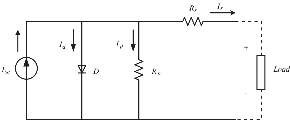
Figure 1: The equivalent circuit of the PV panel

The output power of single PV panel is 213.15 W, the open circuit voltage is 29 V, and the short circuit current is 7.35 A. Fig. 2 shows the current-voltage (I-V) and power-voltage (P-V) characteristics at a constant temperature of 25°C and irradiation of 1000, 8000 and 600 W/m2 for single PV panel. Studies in the literature show that the value of PV voltage under constant temperature scales logarithmically with PV current, which in turn scales linearly with solar irradiation, and as a result, PV voltage increases logarithmically with solar radiation. The effect of solar radiation is much greater in PV current than PV voltage.

I-V and P-V characteristics of the PV panel at constant irradiation and different PV temperatures of 25, 50 and 75°C are shown in Fig. 3. Under constant solar irradiation and different temperature, PV voltage and current are significantly and slightly affected, respectively. PV voltage tends to decrease with increasing temperature.

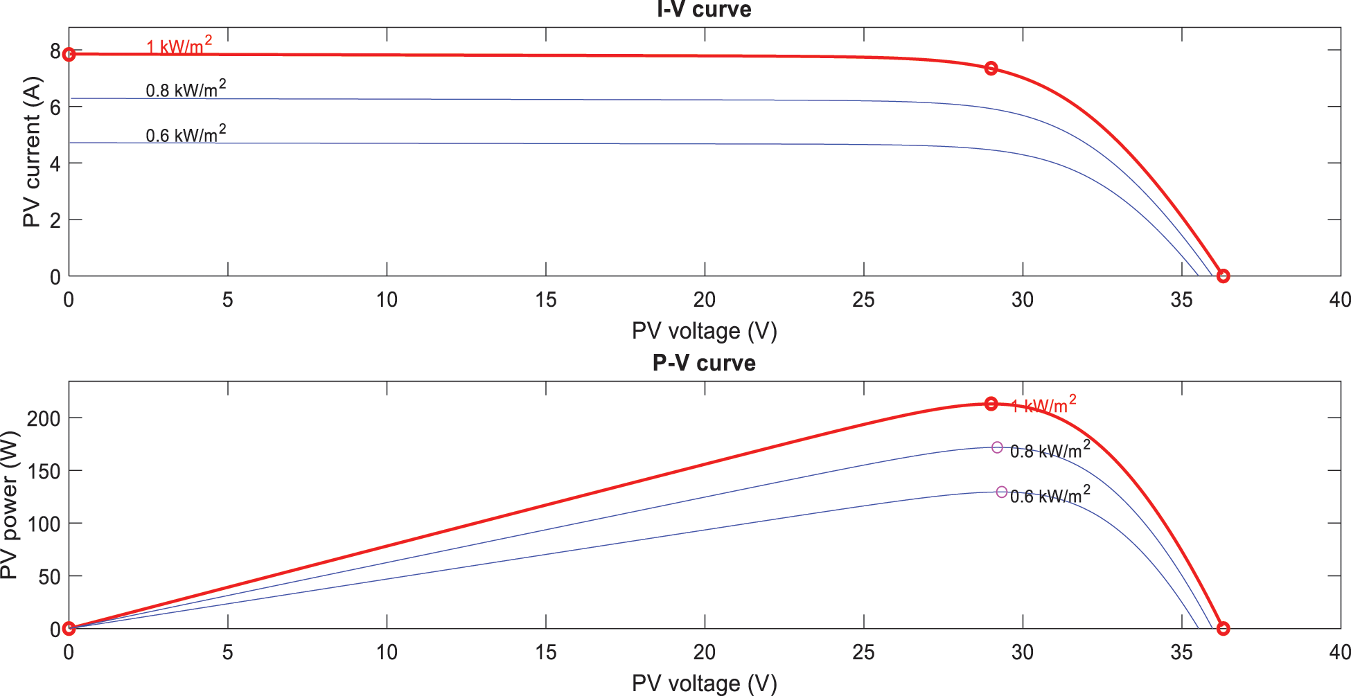
Figure 2: I-V and P-V characteristics of the single PV panel for different solar irradiance

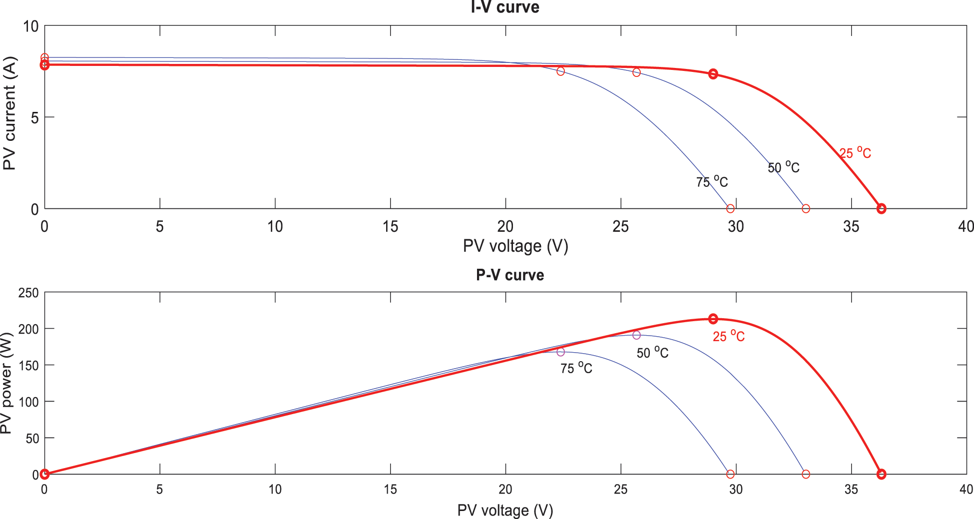
Figure 3: I-V and P-V characteristics of the single PV panel for different PV temperature

The current equation of the PV panel can be achieved as shown in Eq. (10).

I=Iph−Iso(eV+Rs.IVtns−1)−V+Rs.IRsh (10)

The output current is defined by using the parameters, which are the photon current produced in STC ( Iph ), the saturation current ( Iso ), the series resistance and the shunt resistance ( Rs , Rsh ), the quantity of connected cells to the array ( ns ) and the thermal voltage ( Vt ). The thermal voltage is calculated using the Boltzmann's constant K (1.38 × 10−23), the ideal diode factor A , the cell temperature of PV T , the electron charge q (1.602176565 × 10−19). Then, the thermal voltage is expressed as in Eq. (11).

Vt=AKTq (11)

The photon current Iph is defined by using Isc , the current temperature coefficient Ki , light intensity S, and T and it is expressed as in Eq. (12).

Iph=(Isc+Ki(T−298.15))S/100 (12)

The saturation current Iso is defined by the current temperature coefficient, the temperature of cell, the short circuit current, the electron charge, the voltage temperature coefficient Kv , the open-circuit voltage Voc , ideal diode factor, and Boltzmann’s constant as in Eq. (13).

Iso=(Isc+Ki(T−298.15))/(eq(Voc+Kv(T−298.15)AKTns)−1) (13)

2.3 Proposed Kernel Based SVR Maximum Power Prediction Model

The pseudo-code of the of the PV data separating process is presented in Algorithm 1. The pseudo-code of the kernel based SVR forecasting model is presented in Algorithm 2. First, D data are obtained from the PV system and the DC/DC boost converter output. By using a DC/DC boost converter, the maximum power is obtained at the MPP [26]. All the data (D) has a form as shown in Eq. (14).

D=[TGP]1x3 (14)

The input values of the model are defined as panel temperature and solar irradiation, and the output value is defined as the maximum power. T[n] and G[n] are the future data of the PV data, P[n] is the real maximum power output data and fx[n] is the estimated maximum power output data of SVR. Prior to data modeling with statistical method, the normalization technique of the original PV data is a crucial work for a forecasting design. In current study, all the PV data were normalized prior to training and testing to ensure that data are not overwhelmed by each other relating to distance value. The most widely used techniques are Min-Max scaling and Z-score normalization. The Z-score normalization, is generally beneficial in cases where the present minimum and maximum of input data are not known. The normalized data can be achieved as shown in Eq. (15) [27].

Dnorm=(D−μ)/(σ/n) (15)

Here, Dnorm is the normalized values of data, D is the original values of data, μ is the mean of D and σ is the standard deviation of sample means. The μ and σ can be computed by the sample mean and standard deviation statistics, and these two parameters should be saved and used for later prediction. After the implementation of prediction model, the predicted data can be easily reverted to the un-normalized values by using D=(Dnorm∗σ)+μ . The normalized data is divided into training data and test data. The training data is sent to the model to train the kernel-based prediction model and the alpha, weights and bias values are calculated according to the training the model. Using the calculated values and test data, the maximum output power is estimated. The Z-score normalized PV output power is presented in Fig. 4.

3  Case Study and Simulation Results

In the case study, a 2 × 2 PV system was created by connecting 2 panels in series and 2 panels in parallel. In reference to standard test condition, the output power obtained from the system was 852.6 W, the open circuit voltage was 72.6 V, and the short circuit current was 25.68 A. The PV system parameters used in the case study are presented in Tab. 1.

Fig. 5 shows the simulink model of PV panel and DC-DC boost converter developed with the MPP controller. To achieve maximum power in the MPP, a DC-DC boost converter is used due to its low implementation cost, high reliability, and advantage of fewer components. The boost converter consists of an input inductor L placed in series with the output of the PV panel, a semiconductor switch IGBT placed in parallel and a power diode placed in series. In the PV system, different temperatures and different solar irradiation values were applied for estimating the PV maximum power output. Different solar irradiation values were created in MATLAB simulink by using signal builder block for simulated the solar irradiation change for a day.

Figure 4: The Z-score normalized PV output power obtained from the PV system data

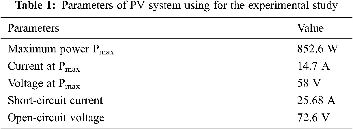
Fig. 6 shows the solar irradiation change curve applied to the PV input. Solar irradiance value increased from 0 to 1000 W/m2. Then, it dropped back to 0. Different temperature values were applied to the PV system between 15 and 40°C using the repeating sequence block as shown in Fig. 7. It produces a linear signal whose minimum value increases from 25°C to a maximum of 40°C for up to 4 s from the start of the simulation.

In this study, the perturb-observe (P&O) algorithm, which produces a slight perturbation at the operating point of the system, is used to obtain the maximum output power in the DC-DC converter circuit. The perturbation causes the PV power to change continuously, and when the power increases due to the perturbation, the perturbation continues in the same direction. The next power decreases after reaching the maximum power point, after which the perturbation reverses. When the maximum power point is reached, the operating point of the system starts to oscillate around the maximum power point continuously. Initially, the power is calculated by measuring the voltage and current of the PV. The derivative of voltage and power is then calculated to determine the change in voltage and power. Then the dP/dV slope is checked under three different conditions. If the slope is dP/dV = 0, the power is at the maximum power point. If the slope is dP/dV > 0, the power is to the left of the maximum power point, and if the slope is dP/dV < 0, the power is to the right of the maximum power point. The controller tracks this maximum point and tries to bring the voltage of the PV to perform on this maximum power point.

Figure 5: The simulink model of PV panel and DC-DC boost converter

Figure 6: The solar irradiation change curve

Fig. 8 presents the power obtained from PV system output and the maximum power obtained from DC/DC boost converter output. As the temperature and solar irradiation value changes, the maximum power obtained from the PV system output changes. Fig. 9 shows the current and voltage signals obtained from PV output and current and voltage signals obtained from DC/DC boost converter output. When different solar irradiation and different temperature inputs are applied at the same time, the voltage will try to increase due to the increase in solar irradiation while the voltage decreases due to the increase in temperature. As a result, the PV voltage will be slightly affected and will not change much. However, PV current will increase by being more affected by solar irradiation and temperature change.

Figure 7: The temperature change curve

Figure 8: The DC/DC boost power and PV power obtained from the PV system output

Figure 9: The current and voltage signals obtained from PV and from DC/DC boost converter

The flow chart of this study is presented in Fig. 10. The maximum power value P were obtained by applying different irradiation G values and different temperature T values in the PV power system consisting of a 2 × 2 PV. When the obtained values were examined, it was seen that the maximum power value changed depending on solar irradiation and temperature and contained information about these values. For the output power alterations, the solar irradiation and the panel temperature can be selected as the input parameters of the maximum power prediction model in PV system. If these parameters change, the maximum power output changes in PV system.

The 1 × 3 dimensional PV data D consists of temperature T, irradiation G and maximum power P values. In current study, all the PV data were normalized. The widely recognized Z-score normalization was utilized as Dnorm. This method was selected due to its successful performance and its frequent reference in literature. By applying preprocessing to the normalized PV data set, all data was separated into test data and training data. To train the proposed prediction model in this study, 80% of the PV data set was used as training data and 20% of the PV data set was used as test data to predict the short term maximum power. The alpha, weights and bias values were calculated according to the training the model. Using the calculated values and test data, the maximum output power was estimated.

To evaluate the performance, the proposed SVR model was utilized in single step very short-term solar prediction and compared to ANN. In addition, some error metrics like Root Mean Square Error (RMSE) and Root Mean Square Error (MSE) were utilized. The performance criteria formulations used are presented in Eqs. (16) and (17).

Figure 10: Flowchart of the proposed kernel based prediction model

MSE=∑i=1N⁡(yi[n]−fx[n])2N (16)

RMSE=∑i=1N⁡(yi[n]−fx[n])2N (17)

where yi[n] is actual values, fx[n] is forecast values of the solar data, N is the total quantity of data. RMSE and MSE were used since they state the total error in solar power output data for the whole data set. The future vectors of the SVR model and ANN model for test data are given in Fig. 11.

The outcomes of performance metrics are given in Tab. 2. They show that there was a considerable betterment in error measurements in comparison to the ANN model and SWD-FFNN. In the short-term power prediction, SVR gave higher prediction performance according to ANN and SWD-FFNN. MSE and RMSE rates which obtained were 4.5566 * 10−04 and 0.0213 using ANN model. MSE and RMSE rates which obtained were 13.0000 * 10−04 and 0.0362 using SWD-FFNN model. Using SVR model, 1.1548 * 10−05 MSE and 0.0034 RMSE rates are obtained. Compared outcomes of the SVR model and ANN model for test data are presented in Fig. 12. Quantities of training and testing data were 3200 and 800, respectively. As stated in Fig. 12, the suggested SVR based model performance increased in cloudy periods.

Figure 11: Future vectors of SVR model ANN model for test data

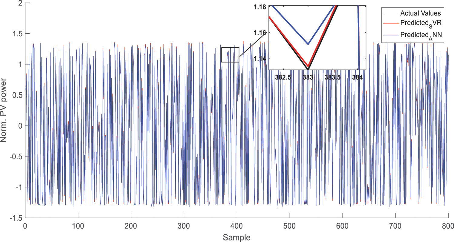
Figure 12: Prediction results of proposed model and ANN model for test data

4  Conclusions

In this study, perturb observation method was applied to obtain maximum power from the PV system at different irradiation and different temperatures, and maximum power was obtained at the output of the boost converter system. In addition, a new power prediction model using a Gaussian kernel based SVR was proposed to estimate the maximum power obtained from the DC-DC boost converter for a short-term. With this model, I aimed to generate a daily forecast by predicting the power values at the MPP during a day’s solar irradiation variation. Short-term PV power prediction is of great importance for optimum operation of grid-connected photovoltaic systems. In the literature, there are only algorithms where the maximum power is obtained at the MPP, and there are only algorithms with short-term power estimation. There are no algorithms where both are made. In this study for the first time in the literature both maximum power is obtained at MPP point and short-term maximum power estimation is made.

The simulated system and data set consists of power data obtained from the maximum power point at one-day variable irradiance and variable temperature value. First, all input data were normalized and were separated as training data and testing data. The normalized data were not affected by each other relating to distance measurement. The normalized data was separated as training data and test data. The training data was sent to the model to train the kernel-based prediction model and the alpha, weights and bias values were calculated according to the training the model. Thus, using the calculated values and test data, the maximum output power is estimated. MSE and RMSE rates which obtained were 4.5566 * 10−04 and 0.0213 using ANN model. MSE and RMSE rates which obtained were 13.0000 * 10−04 and 0.0362 using SWD-FFNN model. Using SVR model, 1.1548 * 10−05 MSE and 0.0034 RMSE rates are obtained. Comparing the two different evaluation statistics RMSE and MSE described above, the simulation results showed that this proposed new kernel based SVR prediction model predicted the PV system maximum output power with higher accuracy at different irradiance and different temperature values compared to ANN and SWD-FFNN are other PV prediction models.

Funding Statement: The author received no specific funding for this study.

Conflicts of Interest: The author declares that I have no conflicts of interest to report regarding the present study.

This work is licensed under a Creative Commons Attribution 4.0 International License, which permits unrestricted use, distribution, and reproduction in any medium, provided the original work is properly cited.