Computer Systems Science & Engineering DOI:10.32604/csse.2022.020448
Article

On Relations for Moments of Generalized Order Statistics for Lindley–Weibull Distribution

Faten A. Momen khan1, Saman Hanif Shahbaz2 and Muhammad Qaiser Shahbaz2,*

1Department of Statistics, University of Jeddah, Jeddah, Kingdom of Saudi Arabia
2Department of Statistics, King Abdulaziz University, Jeddah, Kingdom of Saudi Arabia
*Corresponding Author: Muhammad Qaiser Shahbaz. Email: mkmohamad@kau.edu.sa
Received: 24 May 2021; Accepted: 27 June 2021

Abstract: Moments of generalized order statistics appear in several areas of science and engineering. These moments are useful in studying properties of the random variables which are arranged in increasing order of importance, for example, time to failure of a computer system. The computation of these moments is sometimes very tedious and hence some algorithms are required. One algorithm is to use a recursive method of computation of these moments and is very useful as it provides the basis to compute higher moments of generalized order statistics from the corresponding lower-order moments. Generalized order statistics provides several models of ordered data as a special case. The moments of generalized order statistics also provide moments of order statistics and record values as a special case. In this research, the recurrence relations for single, product, inverse and ratio moments of generalized order statistics will be obtained for Lindley–Weibull distribution. These relations will be helpful for obtained moments of generalized order statistics from Lindley–Weibull distribution recursively. Special cases of the recurrence relations will also be obtained. Some characterizations of the distribution will also be obtained by using moments of generalized order statistics. These relations for moments and characterizations can be used in different areas of computer sciences where data is arranged in increasing order.

Keywords: Generalized order statistics; Lindley–Weibull distribution; recurrence relations; moments

1  Introduction

Several situations arise where the ordering of the data is of great importance. For example arrangement of Olympic records or magnitude of the earthquake measured on a Richter scale etc. The distributional properties of such data are studied by using specialized methods known as ordered random variables. Ordered random variables are classified into several categories but two popular models are order statistics, discussed in detail by [1], and record values, introduced by [2].

Order statistics and record values are special cases of a more general class of models for ordered data, known as generalized order statistics (gos). The gos is a unified model for ordered random variables and has widespread applications in many areas of life. The gos has been introduced by [3] and have been further extended by [4]. The joint density function of gos, introduced by [3], is

fr:n,m~,k(x1,x2,…,xn)=k(∏j=1n−1γj)[1−F(xn)]k−1f(xn)[∏i=1n−1f(xi){1−F(xi)}mi], (1)

where mi, s are constants and m~=(m1,m2,…,mn−1) for n ≥ 2 and γj = k + (n − r) + Mr with Mr=∑j=rn−1mj;1≤r≤n−1 . The marginal distribution of a single gos and joint distribution of two gos have been studied in two different contexts, namely when γi = γj; i ≠ j and when γi ≠ γj; i ≠ j.

The marginal distribution of rth gos when γi = γj; i ≠ j is given by [3] as

fr:n,m,k(x)=Cr−1(r−1)!f(x){1−F(x)}γr−1gmr−1[F(x)] (2)

where Cr−1=∏j=1rγj;r=1,2,…,n , and

gm(x)=hm(x)−hm(0)= { [ 1−(1−x)m+1 ]/(m+1);m≠−1−ln(1−x)m=−1.

The joint density function of two gos for γi = γj is given by [3] as

fr,s:n,m,k(x1,x2)=Cs−1(r−1)!(s−r−1)!f(x1)f(x2){ 1−F(x1) }mgmr−1{ F(x1) }×{ 1−F(x2) }γs−1[ hm{ F(x2) }−hm{ F(x1) } ]s−r−1 ; −∞<x1<x2<∞.(3)

where

hm(x)={ −(1−x)m+1/(m+1) ;m≠−1−ln(1−x)m=−1.

The marginal density function of a single gos and joint density function of two gos when γi ≠ γj; i ≠ j is given by [4] as

fr:n,m~,k(x)=Cr−1f(x)∑i=1rai(r)[1−F(x)]γi−1, (4)

where m~=(m1,m2,…,mn−1) and ai(r)=∏j≠i=1r(γj−γi)−1;1≤i≤r≤n . The joint density of two gos for γi ≠ γj; i ≠ j; is given by [4] as

fr,s:n,m,k(x1,x2)=Cs−1(∑i=r+1sai(r)(s)[F¯(x2)F¯(x1)]γi)(∑i=1rai(r)[F¯(x1)]γi)f(x1)f(x2)F¯(x1)F¯(x2), (5)

for x1 < x2 and ai(r)(s)=∏j≠i=r+1s(γj−γi)−1;r+1≤i≤s≤n . More details about gos can be found in [5,6]. The gos reduces to order statistics if mi = 0 and k = 1 and it reduces to kth record values for mi = −1.

Since the development of gos, several authors have studied the distributional properties of gos for specific probability distributions. Recurrence relations for moments of gos have been an interesting area of research within the domain of gos. Various authors have developed recurrence relations for moments of gos for certain probability distributions. Recurrence relations for moments of gos for a general class of probability distributions have been obtained by [7]. The relations for moments of gos for Marshall–Olkin extended Weibull distribution has been obtained by [8]. The recurrence relations for moments of gos for Kumaraswamy distribution have been obtained by [9]. Reference [10] has obtained relations for moments of gos for a generalized Pareto distribution. The recurrence relations for moments of gos for Kumaraswamy Pareto distribution have been obtained by [11]. Reference [12] has studied the relations for moments of gos for power Lomax distribution whereas the relations for moments of gos for power Lindley distribution have been explored by [13] among others. More details on recurrence relations for moments of gos can be found in [6].

The Weibull distribution, introduced by [14], has been a popular distribution in many areas of life. The distribution has been extended and studied by several authors. The relations for moments of gos for Weibull distribution have been given in [5,6] among others. Recently, [15] has introduced a generalization of Weibull distribution called the Lindley–Weibull distribution. The density and distribution function of the Lindley–Weibull distribution are, respectively

f(x)=βθ2θ+1[αβxβ−1+α2βx2β−1]exp⁡[−θ(αx)β];x,α,β,θ>0 (6)

and

F(x)=1−exp⁡[−θ(αxβ)][1+θθ+1(αx)β];x,α,β,θ>0. (7)

The density and distribution function of the Lindley–Weibull distribution are related as

1−F(x)=[θ+1θ2β∑j=0∞(−1)jαβj−1xβj−β+1+1θβ∑j=0∞(−1)jαβjxβj+1]f(x). (8)

The relation (8) is very useful in recursive computation of moments of gos for the Lindley–Weibull distribution.

We will, now, derive expressions for recursive computation of moments of gos when a sample from the Lindley–Weibull distribution is available. These relations are obtained in the following sections.

2  Recursive Computation of the Simple Moments

The pth moment of gos for a random sample from F(x) is given as

μr:n,m~,kp=∫−∞∞xpfr:n,m~,k(x)dx=∫−∞∞xpCr−1f(x)∑i=1rai(r)[1−F(x)]γi−1dx (9)

These moments are not easy to compute for most of the distribution and hence the recursive computation is used for these moments. An expression for recursive computation of moments of gos for the Lindley–Weibull distribution is given in the following theorem.

Theorem 1: The simple moments of gos for the Lindley–Weibull distribution are related as

μr:n,m~,kp=μr−1:n,m~,kp+pCr−1γrθβ[θ+1θ∑j=0∞(−1)jαβj−1μr:n,m~,kβj−β+p+∑j=0∞(−1)jαβjμr:n,m~,kβj+p]. (10)

Proof: A general relation for recursive computation of moments from any distribution is given by [7] as

μr:n,m~,kp−μr−1:n,m~,kp=pCr−2∫−∞∞xp−1∑i=1rai(r)[1−F(x)]γidx. (11)

The above expression can be written as

μr:n,m~,kp−μr−1:n,m~,kp=pCr−2∫−∞∞xp−1[1−F(x)]∑i=1rai(r)[1−F(x)]γi−1dx.

Now, using (8) in the above equation, we have

μr:n,m˜,kp−μr−1:n,m˜,kp=pCr−1γr∫−∞∞xp−1[ θ+1θ2β∑j=0∞(−1)jαβj−1xβj−β+1+1θβ∑j=0∞(−1)jαβjxβj+1 ]f(x)×∑i=1rai(r)[ 1−F(x) ]γi−1dx

Simplifying and re-arranging the above expression we have

μr:n,m~,kp=μr−1:n,m~,kp+pγrθβ[θ+1θ∑j=0∞(−1)jαβj−1μr:n,m~,kβj−β+p+∑j=0∞(−1)jαβjμr:n,m~,kβj+p],

and hence the result.

Corollary 1: Replacing p with “–p” in (11), the recurrence relation for inverse moments of gos for the Lindley–Weibull distribution is

μr:n,m~,k−p=μr−1:n,m~,k−p−pγrθβ[θ+1θ∑j=0∞(−1)jαβj−1μr:n,m~,kβj−β−p+∑j=0∞(−1)jαβjμr:n,m~,kβj−p]. (12)

Corollary 2: The simple and inverse moments of order statistics for the Lindley–Weibull distribution are related, respectively, as

μr:np=μr−1:np+pθβ(n−r+1)[θ+1θ∑j=0∞(−1)jαβj−1μr:nβj−β+p+∑j=0∞(−1)jαβjμr:nβj+p] (13)

and

μr:n−p=μr−1:n−p−pθβ(n−r+1)[θ+1θ∑j=0∞(−1)jαβj−1μr:nβj−β−p+∑j=0∞(−1)jαβjμr:nβj−p]. (14)

Corollary 3: The simple and inverse moments of kth record values for the Lindley–Weibull distribution are related, respectively, as

μK(r)p=μK(r−1)p+pθβk[θ+1θ∑j=0∞(−1)jαβj−1μK(r)βj−β+p+∑j=0∞(−1)jαβjμK(r)βj+p], (15)

and

μK(r)−p=μK(r−1)−p−pθβk[θ+1θ∑j=0∞(−1)jαβj−1μK(r)βj−β−p+∑j=0∞(−1)jαβjμK(r)βj−p], (16)

3  Recursive Computation of the Joint Moments

The (p, q)th moment of gos for a random sample from F(x) is given as

μr,s:n,m˜,kp,q=∫−∞∞∫x1∞x1px2qfr,s:n,m˜,k(x)dx2dx1                  =∫−∞∞∫x1∞x1px2qCs−1(∑i=r+1sai(r)(s)[ F¯(x2)F¯(x1) ]γi)(∑i=1rai(r)[ F¯(x1) ]γi)f(x1)f(x2)F¯(x1)F¯(x2)dx2dx1.

In the following, we will obtain an expression for recursive computation of product moments of gos for the Lindley–Weibull distribution.

Theorem 2: The product moments of gos for the Lindley–Weibull distribution are related as

μr,s:n,m~,kp,q=μr,s−1:n,m~,kp,q+qγrθβ[∑j=0∞(−1)jαβj−1{θ+1θμr,s:n,m~,kp,βj−β+q+αμr,s:n,m~,kp,βj+q}]. (17)

Proof: Following [6], a relation for recursive computation of product moments from any distribution is

μr,s:n,m~,kp,q−μr,s−1:n,m~,kp,q=qCs−2∫−∞∞∫x1∞x1px2q−1(∑i=r+1sai(r)(s)[F¯(x2)F¯(x1)]γi)×(∑i=1rai(r)[F¯(x1)]γi)f(x1)F¯(x1)dx2dx1. (18)

The above expression can be written as

μr,s:n,m~,kp,q−μr,s−1:n,m~,kp,q=qCs−2∫−∞∞∫x1∞x1px2q−1(∑i=r+1sai(r)(s)[F¯(x2)F¯(x1)]γi)(∑i=1rai(r)[F¯(x1)]γi)×f(x1)F¯(x1)F¯(x2)F¯(x2)dx2dx1.

Now, using (8) in the above equation, we have

μr,s:n,m~,kp,q−μr,s−1:n,m~,kp,q=qCs−1γs∫−∞∞∫x1∞x1px2q−1(∑i=r+1sai(r)(s)[F¯(x2)F¯(x1)]γi)(∑i=1rai(r)[F¯(x1)]γi)×f(x1)f(x2)F¯(x1)F¯(x2)[1θβ∑j=0∞(−1)jαβj−1{θ+1θx2βj−β+1+αx2βj+1}]dx2dx1.

Simplifying the above expression we have

μr,s:n,m~,kp,q=μr,s−1:n,m~,kp,q+qγsθβ[∑j=0∞(−1)jαβj−1{θ+1θμr,s:n,m~,kp,βj−β+q+αμr,s:n,m~,kp,βj+q}],

and hence the result.

Corollary 4: The recursive relation for ratio moments of gos for the Lindley–Weibull distribution is

μr,s:n,m~,kp,−q=μr,s−1:n,m~,kp,−q−qγrθβ[∑j=0∞(−1)jαβj−1{θ+1θμr,s:n,m~,kp,βj−β−q+αμr,s:n,m~,kp,βj−q}]. (19)

Corollary 5: The joint and ratio moments of order statistics for the Lindley–Weibull distribution are related as

μr,s:np,q=μr,s−1:np,q+qθβ(n−s+1)[∑j=0∞(−1)jαβj−1{θ+1θμr,s:np,βj−β+q+αμr,s:np,βj+q}] (20)

and

μr,s:np,−q=μr,s−1:np,−q−qθβ(n−s+1)[∑j=0∞(−1)jαβj−1{θ+1θμr,s:np,βj−β−q+αμr,s:np,βj−q}]. (21)

Corollary 6: The joint and ratio moments of kth records for the Lindley–Weibull distribution are related as

μK(r,s)p,q=μK(r,s−1)p,q+qθβk[∑j=0∞(−1)jαβj−1{θ+1θμK(r,s)p,βj−β+q+αμK(r,s)p,βj+q}] (22)

and

μK(r,s)p,−q=μK(r,s−1)p,−q−qθβk[∑j=0∞(−1)jαβj−1{θ+1θμK(r,s)p,βj−β−q+αμK(r,s)p,βj−q}]. (23)

4  Characterizations

In this section, we will give some characterizations for the Lindley–Weibull distribution in terms of simple and product moments of gos. These characterizations are given when mi = m and in this case, the relation (11) reduces to

μr:n,m,kp−μr−1:n,m,kp=pCr−1γr(r−1)!∫−∞∞xp−1[F¯(x)]γrgmr−1[F(x)]dx, (24)

where F¯(x)=1−F(x). The relation (21) will be helpful to obtain the characterizations. The characterizations are given in the following theorems.

Theorem 3: A necessary and sufficient condition for a random variable X to have density and distribution functions (6) and (7) respectively is that the moments of its gos are related as

μr:n,m,kp−μr−1:n,m~,kp=pγrθβ[∑j=0∞(−1)jαβj−1{θ+1θμr:n,m~,kβj−β+p+αμr:n,m~,kβj+p}].

Proof: The necessary condition immediately follows from Theorem 1. To prove the sufficient condition consider the relation (21) and hence we have

pCr−1γr(r−1)!∫−∞∞xp−1[F¯(x)]γrgmr−1[F(x)]dx=pγrθβ[∑j=0∞(−1)jαβj−1{θ+1θμr:n,m~,kβj−β+p+αμr:n,m~,kβj+p}]

or

pγrCr−1(r−1)!∫0∞xp−1[F¯(x)]γrgmr−1[F(x)]dx=pγrθβ[∑j=0∞(−1)jαβj−1×Cr−1(r−1)!∫0∞xp−1{F¯(x)}γr−1gmr−1{F¯(x)}{θ+1θxβj−β+1+αxβj+1}f(x)dx]

or

pγrCr−1(r−1)!∫0∞xp−1[F¯(x)]γr−1gmr−1[F(x)][F¯(x)−1θβ∑j=0∞(−1)jαβj−1{θ+1θxβj−β+1+αxβj+1}f(x)]dx=0

Using Müntz–Száz; see [16]; to above equation we have

F¯(x)=[1θβ∑j=0∞(−1)jαβj−1{θ+1θxβj−β+1+αxβj+1}]f(x),

which is (8) and hence the theorem.

Theorem 4: A necessary and sufficient condition for a random variable X to have density and distribution functions (6) and (7) respectively is that the product moments of its gos are related as

μr,s:n,m,kp,q−μr,s−1:n,m,kp,q=qγrθβ[∑j=0∞(−1)jαβj−1{θ+1θμr,s:n,m,kp,βj−β+q+αμr,s:n,m,kp,βj+q}]. (25)

Proof: The necessary part immediately follows from Theorem 2. For sufficient part, we consider the following relation between product moments of gos for any distribution F(x) when mi = m, given by [7],

μr,s:n,m,kp,q−μr,s−1:n,m,kp,q=qCs−1γs(r−1)!(s−r−1)!∫−∞∞∫x1∞x1px2q−1f(x1)[F¯(x1)]mgmr−1[F(x)]×[hm{F(x2)}−hm{F(x1)}]s−r−1[F¯(x2)]γsdx2dx1.

Now using the above relation in (22) we have

qCs−1γs(r−1)!(s−r−1)!∫0∞∫x1∞x1px2q−1f(x1)[F¯(x1)]mgmr−1[F(x1)][hm{F(x2)}−hm{F(x1)}]s−r−1×[F¯(x2)]γsdx2dx1=qγsθβ[θ+1θ∑j=1n(−1)jαβj−1Cs−1(r−1)!(s−r−1)!∫0∞∫x2∞x1px2q−1f(x1){F¯(x1)}m× gmr−1{F(x1)}{hm(F(x2))−hm(F(x1))}s−r−1{F(x)}γs−1{θ+1θx2βj−β+1+αx2βj+1}dx2dx1]

or

qCs−1γs(r−1)!(s−r−1)!∫0∞∫x1∞x1px2q−1f(x1)[F¯(x1)]mgmr−1[F(x1)][hm{F(x2)}−hm{F(x1)}]s−r−1×[F¯(x2)]γs−1[F¯(x2)−1θβ∑j=1n(−1)jαβj−1{θ+1θx2βj−β+1+αx2βj+1}f(x2)]dx2dx1=0

Using Müntz–Száz; see [16]; to above equation we have

F¯(x2)=1θβ∑j=1n(−1)jαβj−1{θ+1θx2βj−β+1+αx2βj+1}f(x2),

which is (8) and hence the theorem.

5  Numerical Study

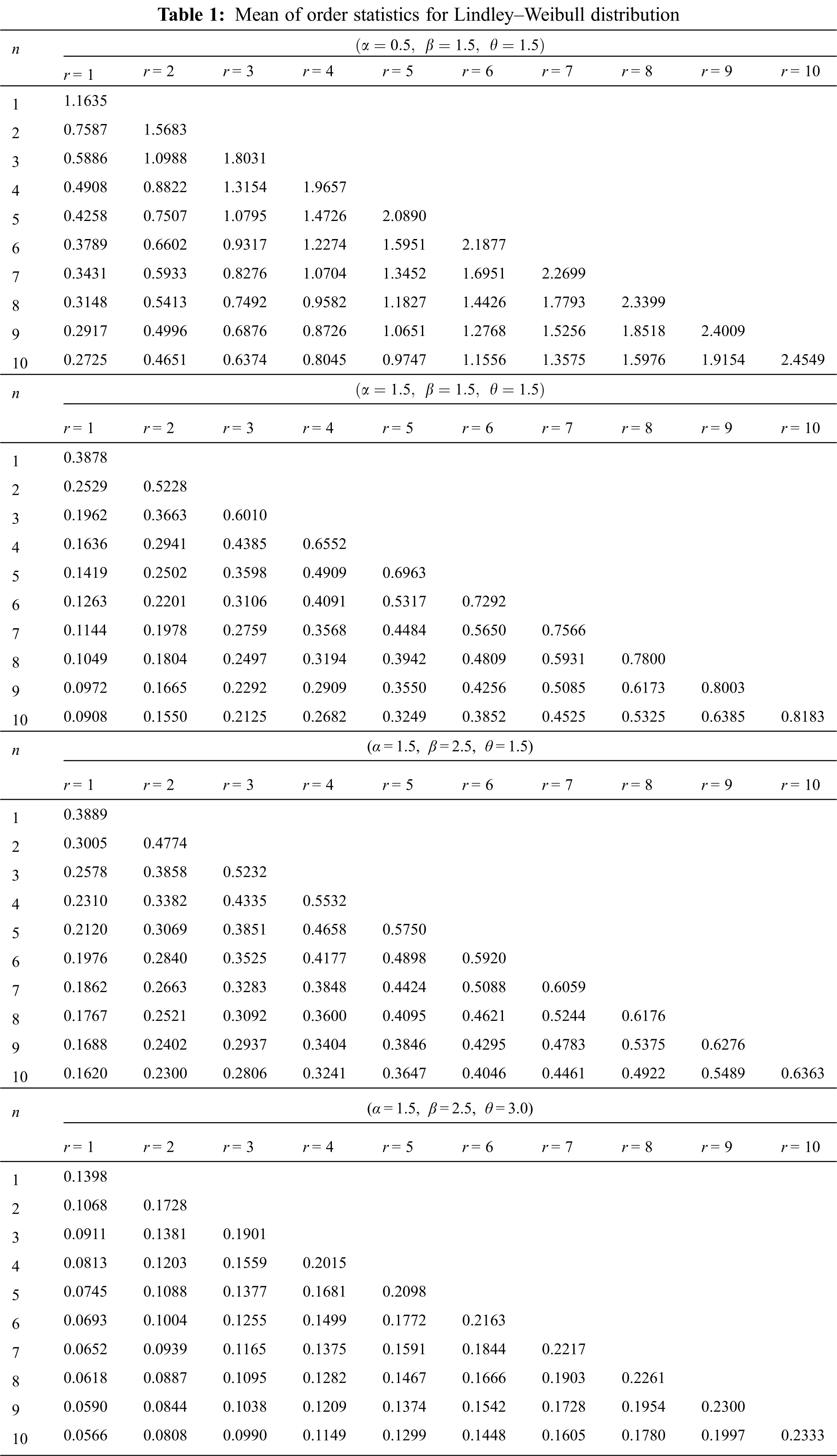
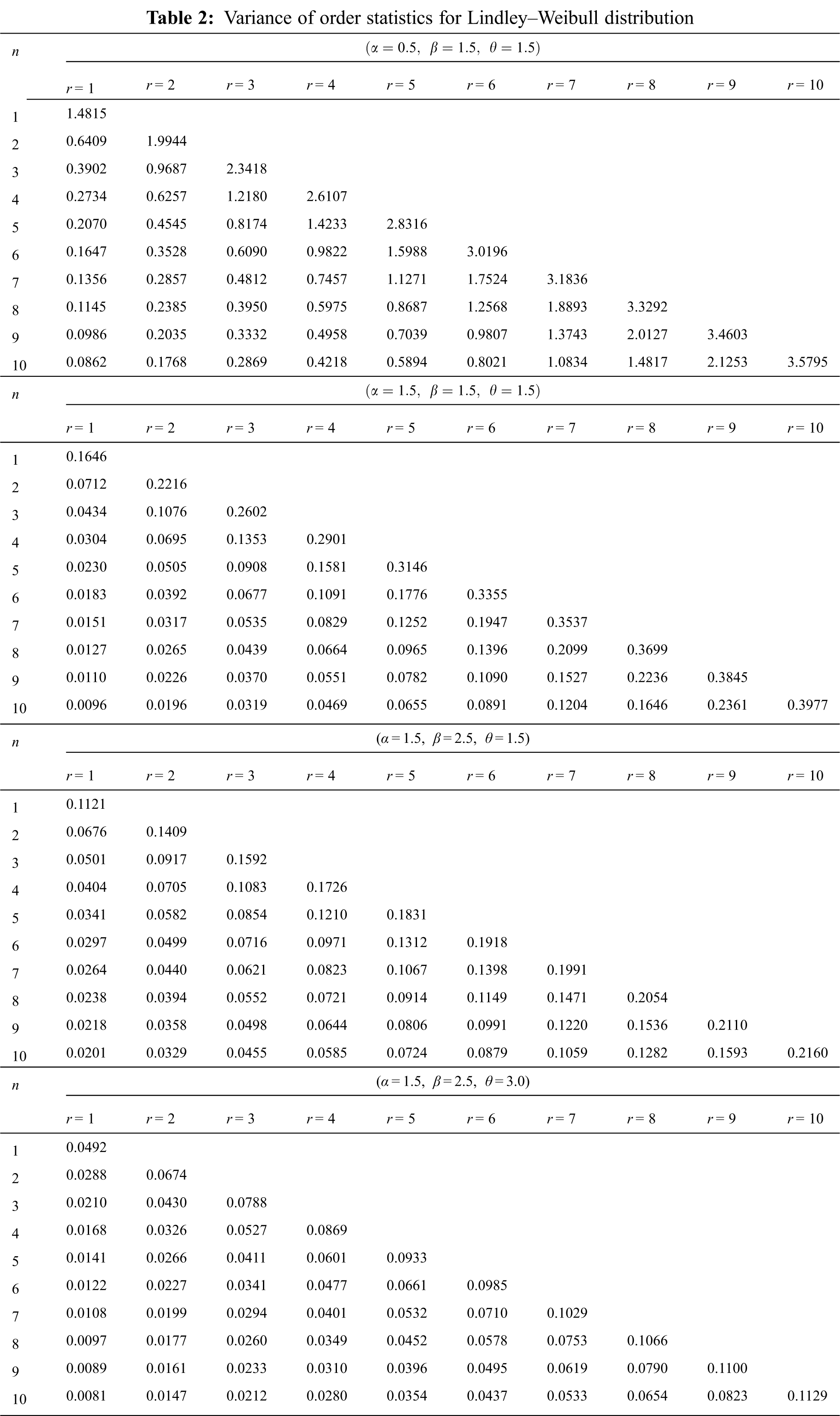
In this section, we have given the numerical study for moments of order statistics when the sample is available from the Lindley–Weibull distribution. We have computed mean and variance of order statistics for the Lindley–Weibull distribution using various combinations of parameters. The results are given in Tabs. 1 and 2 in Appendix A.

Tab. 1 contains mean of order statistics for the Lindley–Weibull distribution for various combinations of the parameters. From this table we can see that, for fixed α, β, θ and n, the mean of order statistics increases with an increase in the value of r. Also for fixed α, β, θ and r the mean of order statistics decreases with an increase in the value of n. Further, from Tab. 1, we can see that for fixed β, θ, n and r the mean of order statistics decreases with an increase in the value of α and for fixed values of α, β, n and r the mean decreases with increase in θ. This table also shows an interesting effect of the parameter β on the mean of order statistics. We can see from this table that for fixed α, θ, n and increase in β, the mean increases for r ≤ (n + 1)/2 + 1 and decreases for r > (n/2) + 2.

Tab. 2 contains variances of order statistics for the Lindley–Weibull distribution for various combinations of parameters. The effect of α, θ, n and r on variance are the same as their effect on the mean. We can see from this table that for fixed α, θ, n and increase in β the variance increases for r ≤ (n − 1)/2 + 1 and decreases for r > (n/2) − 2.

6  Conclusions

In this paper, we have derived expressions for recursive computation of single, product, inverse and ratio moments of gos when the sample is available from the Lindley–Weibull distribution. The derived relations provide relations for moments of order statistics and record values as a special case. These relations are useful to compute the moments for any value of the parameters. The mean and variance of order statistics for the Lindley–Weibull distribution are computed for different values of parameters. It is observed that for fixed n the mean and variance of order statistics increases with an increase in r and for fixed r the mean and variance decreases with an increase in n. We have also obtained the characterizations of the Lindley–Weibull distribution using single and product moments of gos.

Funding Statement: The work was funded by the University of Jeddah, Saudi Arabia under Grant Number UJ–02–093–DR. The authors, therefore, acknowledge with thanks the University for technical and financial support.

Conflicts of Interest: The authors declare that they have no conflicts of interest to report regarding the present study.

Appendix A

This work is licensed under a Creative Commons Attribution 4.0 International License, which permits unrestricted use, distribution, and reproduction in any medium, provided the original work is properly cited.