Computer Systems Science & Engineering DOI:10.32604/csse.2022.020590
Article

Adaptive Scheme for Crowd Counting Using off-the-Shelf Wireless Routers

Wei Zhuang1,2, Yixian Shen1, Chunming Gao3, Lu Li1, Haoran Sang4 and Fei Qian5,*

1School of Computer and Software, Nanjing University of Information Science & Technology, Nanjing, 210044, China
2Engineering Research Center of Digital Forensics, Ministry of Education, Nanjing University of Information Science and Technology, Nanjing, 210044, China
3School of Engineering & Technology, University of Washington, Tacoma, WA 98402, USA
4China General Nuclear Power Group, Nanjing, 210028, China
5Jiangsu Province Hospital of Chinese Medicine, Affiliated Hospital of Nanjing University of Chinese Medicine, Nanjing, 210029, China
*Corresponding Author: Fei Qian. Email: seujaguar@163.com
Received: 29 May 2021; Accepted: 30 June 2021

Abstract: Since the outbreak of the world-wide novel coronavirus pandemic, crowd counting in public areas, such as in shopping centers and in commercial streets, has gained popularity among public health administrations for preventing the crowds from gathering. In this paper, we propose a novel adaptive method for crowd counting based on Wi-Fi channel state information (CSI) by using common commercial wireless routers. Compared with previous researches on device-free crowd counting, our proposed method is more adaptive to the change of environment and can achieve high accuracy of crowd count estimation. Because the distance between access point (AP) and monitor point (MP) is typically non-fixed in real-world applications, the strength of received signals varies and makes the traditional amplitude-related models to perform poorly in different environments. In order to achieve adaptivity of the crowd count estimation model, we used convolutional neural network (ConvNet) to extract features from correlation coefficient matrix of subcarriers which are insensitive to the change of received signal strength. We conducted experiments in university classroom settings and our model achieved an overall accuracy of 97.79% in estimating a variable number of participants.

Keywords: CSI; device-free; deep learning; crowd counting; Wi-Fi; wireless sensing

1  Introduction

Wi-Fi has gained an increasing interest in research due to the implementation of orthogonal frequency-division multiplexing (OFDM) and multiple-input multiple-output (MIMO) technology. In telecommunication with high throughput and multiantenna, the channel state information (CSI) can make the transmissions adapt to current channel condition, which is of great significance. CSI characterizes how wireless signals propagate from the transmitter to the receiver at certain carrier frequency of certain communication link. Each CSI entry represents the channel frequency response (CFR), which is shown in Eq. (1).

H(f;t)=∑iN⁡ai(t)e−j2πfτi(t) (1)

where, ai(t) is the amplitude attenuation factor, τi(t) is the propagation delay, and f is the frequency of carrier. For each subcarrier of one link, the channel can be modeled by y=Hx+n , where, y is the received signal, x is the transmitted signal, H is the CSI matrix, and n is the environment noise. In this paper, the CSI matrix H is estimated at the receiver side by evaluating the difference between the pre-defined transmitted signal x and received signal y after OFDM demodulation using the Atheros CSI Tool [1].

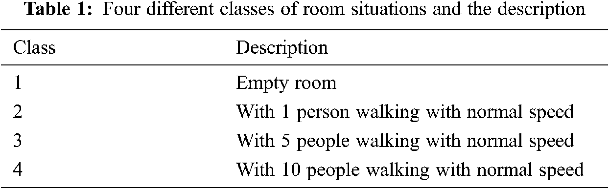
Wireless sensing based on Wi-Fi signals has caught tremendous attentions due to its ubiquity and privacy-preserving features [2–8]. Many researchers have paid much attention on human crowd counting based on the widely deployed wireless routers in public areas. Human crowd count estimation has also attracted increasing attention in many potential applications, such as intelligent surveillance, crowd management, urban security and business decision-making etc. For example, the accurate human population distribution information of one city can bring benefit for the government management personnel to make population-related decisions more efficiently. Since the outbreak of the world-wide novel coronavirus pandemic, crowd counting in public areas, such as in shopping centers and in commercial streets, has gained popularity among public health administrations for preventing the crowds from gathering. Traditionally, image-based methods are most often used to estimate the human crowd count, but they are limited to the illumination intensity of environment, line-of-sight propagation property of light, and the public consideration of privacy [9–18]. In this paper, we introduce an adaptive model for human crowd count estimation by exploiting rich CSI data embedded in 802.11n Wi-Fi networks. To test the robustness of the proposed model, we evaluated its performance in four different scenarios, which are shown in Tab. 1.

The CSI data is collected from the AR9344 NIC which is embedded in TP-LINK WDR4310 wireless router based on the Atheros CSI Tool.

After collecting the raw CSI data, Kalman filter with Mahalanobis Distance is used to detect abnormality and smooth out the signal [19–20]. Then, the correlation coefficient matrix of subcarriers is calculated for each data link to generate images. In order to extract fine features of the images, convolutional neural network (ConvNet) is used and the trained classification model achieves a satisfying result on the evaluation dataset in the four scenarios [21].

The remainder of the paper is structured as follows. The Section 2 presents the background and related works of crowd counting and Wi-Fi based wireless sensing. The Section 3 presents the system procedure of human crowd counting system, including data collection and analysis, data preprocessing, feature extraction, and construction of classification model. The Section 4 presents the implementation and evaluation of crowd counting system. The Section 5 presents the conclusion.

2  Background and Related Works

In 2015, Gong et al. [22] designed a Wi-Fi-based real-time calibration-free passive human motion detection system based on the physical layer information using two schemes: short-term averaged variance ration (SVR) and long-term averaged variance ration (LVR). According to the experiment result, a high detection rate and low false positive rate are achieved. In 2016, Domenico et al. [23] proposed one trained-once device-free crowd counting and occupancy estimation using Wi-Fi based on a Doppler spectrum approach in WiMob. The proposed approach analyzes the linear correlation relationship between the shape of the Doppler spectrum and the received signal. In 2017, Zhu et al. [24] proposed an abnormal activity detection system NotiFi which achieved satisfactory performance in accuracy, robustness, and stability. It is based on the fact that the amplitude and phase information of CSI change sensitively whenever the human body occludes the wireless signal from the access point (AP) to the monitor point (MP). Yen-Kai et al. extends crowd counting technique to people-centric Internet of Things (IoT) applications, e.g., security monitoring and energy management for smart homes based on fine-grained physical-layer wireless signatures. They achieved an average correct classification rate of 88% in estimating the exact number of the crowd of size up to nine people in general indoor scenarios. In 2014, Xi et al. [25] proposed the Percentage of nonzero Elements (PEM), in the dilated CSI Matrix, and then the monotonic relationship was explicitly formulated by the Grey Verhulst Model. In 2019, Ibrahim et al. [26] proposed CROSS-COUNT, which uses a single Wi-Fi link to estimate the human crowd count based on the temporal link-blockage pattern and achieves a high accuracy with non-labor-intensive data.

3  System Procedure of Human Crowd Count Estimation

3.1 Data Collection and Analysis

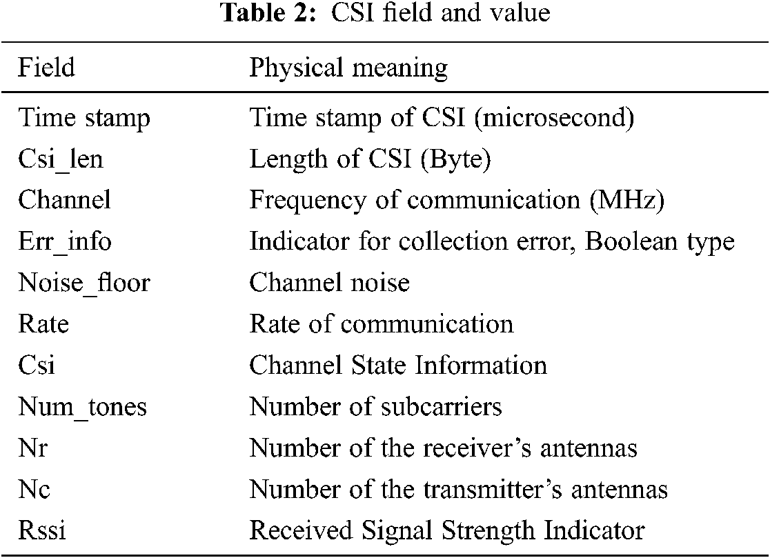
Each CSI measurement contains several fields, which are shown in Tab. 2.

Each CSI measurement is a Nr×Nc×Numtones three-dimensional tensor, where Nr denotes number of antennas of the receiver, Nc denotes number of antennas of the sender, and Numtones denotes number of subcarriers in the frequency band used for communication in the experiment. In this experiment, the configuration Nr=2,Nc=2,andNumtones=56 . The sampling frequency is 30 Hz, and the sampling duration of each group is 60 s. The experiment was conducted in four different room situations, with the room being empty, with 1 person walking at normal speed, with 5 people walking at normal speed, and with 10 people walking at normal speed. A total of four groups of CSI data were collected and each group contains 1,800 CSI measurements. Fig. 1 shows the amplitude change of 56 subcarriers of 300 CSI packets in empty room situation. Fig. 2 shows the amplitude change of four different communication links between AP and MP of a single subcarrier in empty room situation.

Figure 1: Amplitude of 56 subcarriers of 300 CSI packets in empty room

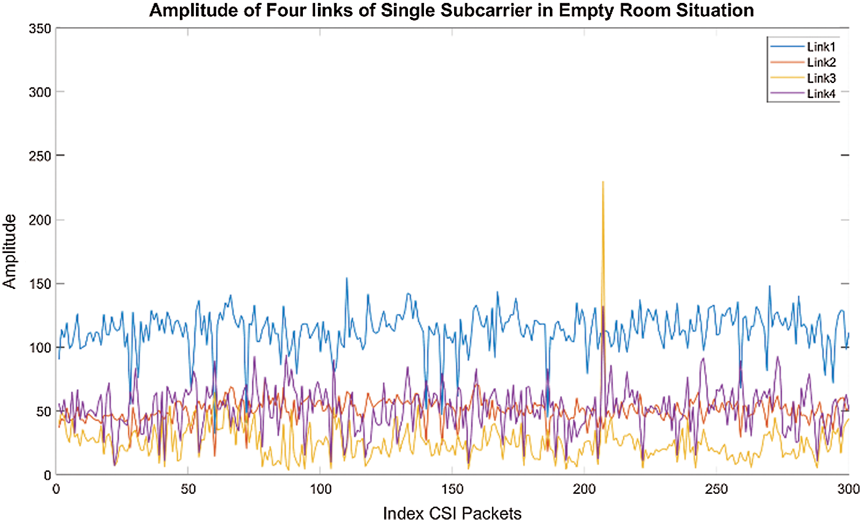
Figure 2: Amplitude of four links of single subcarrier in empty room

3.2 Data Preprocessing

Generally, the collected CSI is an estimate of the wireless channel and contains random noise and other inaccuracies. In order to have a better estimate of the wireless channel based on the collected CSI, in this paper, Kalman Filter is used to filter noise and remove outliers. It can be seen in Eqs. (2) and (3).

x(t)=Ax(t−1)+B(t)u(t)+w(t) (2)

y(t)=Cx(t)+v(t) (3)

where, A is one-dimensional state transition matrix and A = [ [1.0]] is implemented in our case. B(t) is the influence of the control action at time t , and u(t) is the control vector at time t . In our case, B(t) and u(t) are not implemented. w(t) is the process noise at time t , C is the observation matrix which maps the true state space into the measured space, v(t) is the measurement noise at time t , x(t) is the estimated system state at time t derived from the state at time t−1 , and y(t) is the measurement at time t . w(t)andv(t) are assumed to be drawn from zero mean normal distribution N(0,Rww) and N(0,Rvv) respectively, where Rww denotes covariance of process noise and Rvv denotes covariance of measurement noise.

The Kalman filter can be divided into two procedures: “Prediction” and “Update”.

Prediction procedure using Eqs. (4) and (5):

x^(t|t−1)=A(t−1)x^(t−1|t−1)+B(t)u(t) (4)

P^(t|t−1)=A(t−1)P^(t−1|t−1)A(t−1)T+Rww(t) (5)

where, x^(t|t−1) is the priori estimated state of system at time t given measurement at time t−1 , A(t−1) is the state transition model at time t−1 applied to the previous posteriori estimated state x^(t−1|t−1) , P^(t|t−1) is the priori estimated covariance, and Rww(t) is the covariance of process noise at time t . The priori state of current time is estimated using the posteriori estimated state from the previous time in the prediction procedure.

Update procedure Eqs. (6)–(10):

e(t)=y(t)−C(t)x^(t|t−1) (6)

Ree(t)=C(t)P^(t|t−1)C(t)T+Rvv(t) (7)

K(t)=P^(t|t−1)C(t)TRee(t)−1 (8)

x^(t|t)=x^(t|t−1)+K(t)e(t) (9)

P^(t|t)=(I−K(t)C(t))P^(t|t−1) (10)

where, e(t) denotes the innovation, Ree(t) denotes the innovation covariance, K(t) denotes the optimal Kalman gain, x^(t|t) denotes the posteriori updated state, and P^(t|t) denotes the posteriori updated estimate covariance.

Since only the current measurement and the estimated state from the previous time are required to compute the estimate for the current state, Kalman filter is a computationally efficient algorithm for real-time and light-weight applications.

In order to detect and remove outliers, Weighted Mahalanobis Distance MD(t) of a given measurement y(t) and a predicted value x^(t|t−1) are used in this paper. As shown in Eq. (11):

MD(t)=(y(t)−x^(t|t−1))TRee−1(y(t)−x^(t|t−1)) (11)

Rvv=Δ1+e−MD(t)+ξ (12)

where, Δ and ξ are constants, which can be determined by analyzing the statistical feature of the signal.

The Rvv can be considered as how much the system can trust on the measurement. The bigger the Rvv value is, the less trust the system will have on the measurement. The value of Rvv can be adaptively updated based on the amount of noise suffered according to Eq. (12) above.

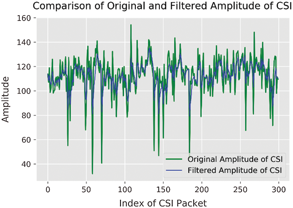
Figure 3: Comparison of original and filtered amplitude of CSI

The amplitudes before and after Kalman filtering of the first subcarrier of link 1 in the empty room situation are shown in Fig. 3.

3.3 Feature Extraction

The correlation coefficient matrix is calculated using Eq. (13).

M=[1Cof(1,2)⋯Cof(1,n)Cof(2,1)1⋯Cof(2,n)⋮⋮⋱⋮Cof(n,1)Cof(n,1)⋯1] (13)

where, Cof(i,j) means the Pearson Correlation Coefficient of ith subcarrier and jth subcarrier, which is calculated using Eq. (14):

ρX,Y=cov(X,Y)σXσY (14)

where, cov is the covariance, σX is the standard deviation of X , and σY is the standard deviation of Y . The Pearson Correlation Coefficient measures linear combination between two variables X and Y which has a value between −1 and +1. A value of −1 means totally negative linear correlation, 0 means no linear correlation between X and Y , and +1 means total positive linear correlation.

Considering the tasks of recognizing the number of people in a room, the window size W=10s and step size S=0.5s were selected when using the sliding window size method to produce the samples of each scenario for classification. The total number of CSI measures of one scenario is N=1800 and a total number of (N−W)/S+1=108 windows can be generated from the collected data of one scenario.

In this paper, only the amplitude information of CSI is used, as the amplitude correlation of subcarriers is sensitive to the number change of people in a closed room based on the experiment. The data shape of single window is Nr×Nc×Numtones×W , which is 2×2×56×300 in this case. For simplicity, select the first antenna of receiver and the first antenna of sender in the beginning and apply the same method to the other three links later. Calculate the Person Correlation Coefficient of any two subcarriers in one window according to Eq. (14).

Generate gray level image with 56×56 pixels from correlation coefficient matrix M . The gray level image of four different classes is shown in Fig. 4. Since there are 2×2 links, the total number of images generated from the collected data is 2×2×108×4=1728 .

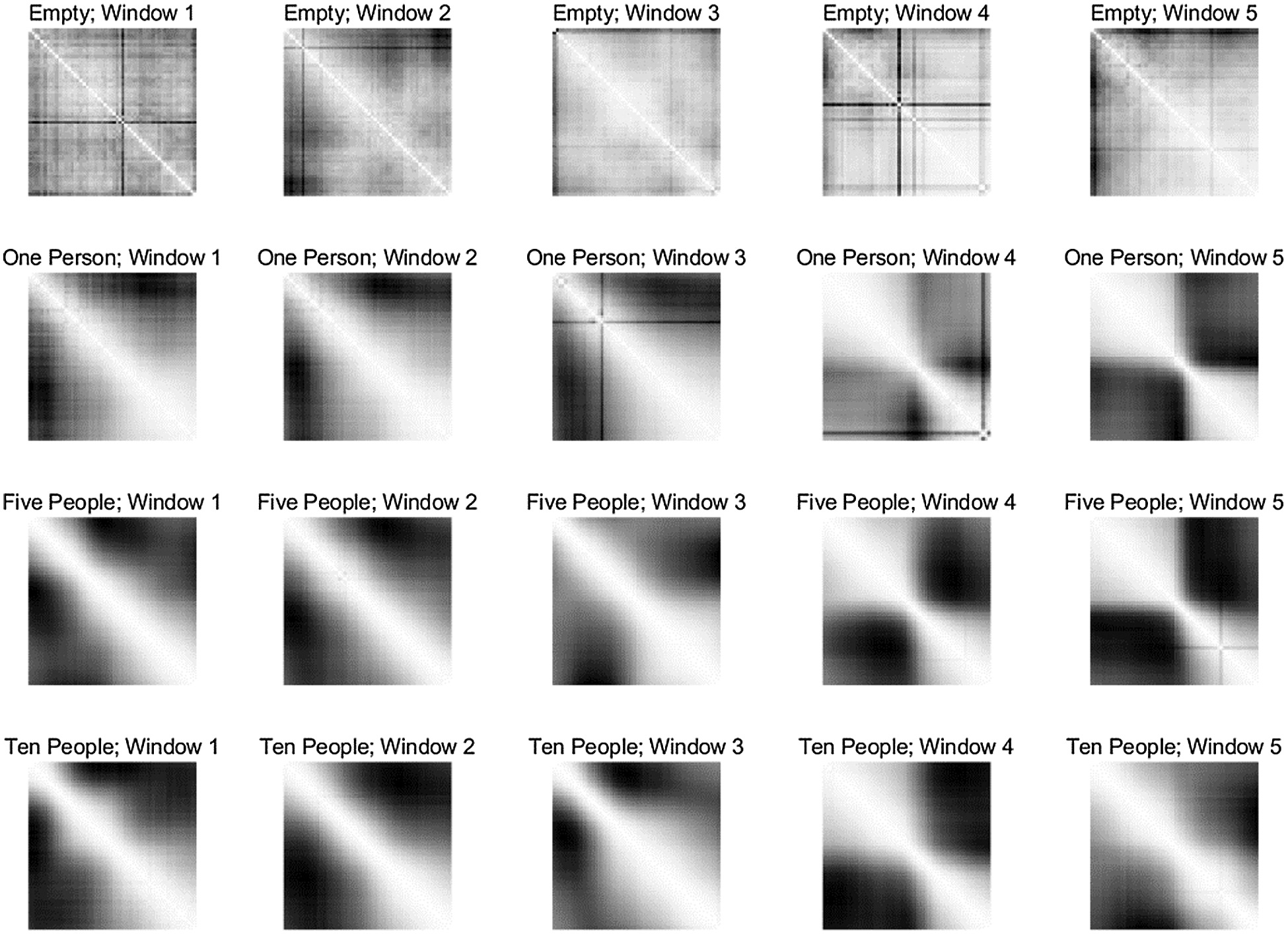
Figure 4: Image of correlation coefficient matrix of four different classes

3.4 Construction of ConvNet Classification Model

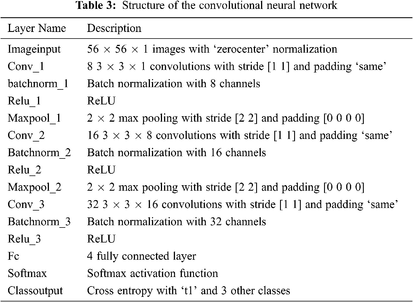
The structure of ConvNet constructed in this paper is shown in Tab. 3.

3.5 Description of Convnet’s Layers and Parameters

3.5.1 The Convolutional Layer

The input is a tensor with shape (NI×HI×WI×DI) , where NI is the number of images, HI is the height of the image, WI is the width of the image, and DI is the depth of the image. After passing through a convolutional layer, the tensor becomes abstracted to a feature map with shape (NI×FHI×FWI×FCI) , where FHI is the feature map height, FWI is the feature map width, and FCI is the feature map channels. The shape of convolutional kernel is 3×3 for all three convolutional layers and the number of input channels and output channels are (1,8) , (8,16) , (16,32) for conv_1, conv_2, and conv_3 respectively.

3.5.2 The Polling Layer

Pooling is a form of non-linear down-sampling, which partitions the input image into a set of non-overlapping sub-regions. The max pooling unit uses the function f=max(A(1,1),A(1,2),...,A(m,n)) , where A denotes the matrix of the sub-region with shape m by n , to generate single value from the partitioned sub-region. Pooling layer can decrease the spatial size of image and reduce the number of parameters significantly. Commonly, the filter with size 2×2 and a stride of 2 along both width and height is selected, and 75% of the activations will be discarded.

3.5.3 The Relu Layer

The rectifier is an activation function defined as Eq. (15).

f(x)=max(0,x) (15)

It maps negative values to zero and keeps the non-negative values unchanged. The rectified linear unit increases the nonlinear properties of the decision function.

3.5.4 The Learning Rate

Learning rate is a hyperparameter in an optimization algorithm, which determines the step size at each iteration while moving towards a minimum of the cost function. A high learning rate will probably make the learning jump over the minima. On the opposite, a low learning rate generally takes too much time to converge and even makes the learning progress stuck in the local minimum. Therefore, there should be a trade-off when selecting the learning rate for a specific problem. In this paper, a common value 0.01 of learning rate was selected when training the ConvNet.

3.5.5 Batch Normalization

Batch normalization is a method which uses re-centering and re-scaling to accelerate the training progress and make the neural network more stable. The batch normalization improves the performance by smoothing the objective function.

Batch normalization fixes the means and variances of the inputs of each layer. μB=1m∑i=1m⁡xi , σB2=1m∑i=1m⁡(xi−μB)2 , where B denotes the mini-batch of size m of the entire training set, μB denotes the mean of mini-batch B , and σB2 denotes the variance of mini-batch B . For a ConvNet, whose input layer has the shape (NI×HI×WI×DI) , the batch normalization procedure is shown in Eqs. (16) and (17), and each element in the matrix x should be normalized separately.

x=[x(1,1)x(1,2)⋯x(1,WI)x(2,1)x(2,2)⋯x(2,WI)⋮⋮⋱⋮x(HI,1)x(HI,2)⋯x(HI,WI)] (16)

x^i(j,k)=xi(j,k)−μB(j,k)σB2(j,k)+ϵ (17)

where j∈[1,WI],k∈[1,HI]andi∈[1,m] ; μB(j,k) and σB2(j,k) are the mean and variance of each element in the matrix x respectively; ϵ is an arbitrarily small constant added for numerical stability. In the end, the x^i(j,k) will have zero mean and unit variance.

3.5.6 Softmax Function

SoftMax function is a generalized multiple dimensions version of logistic function which is a common S-shape curve. The equation of logistic function is f(x)=L1+e−k(x−x0) , where x0 is the value of the midpoint, L is the curve’s maximum value and k is the logistic steepness of the curve. When x0=0,L=1,k=1 , f(x) is the standard logistic function. Similarly, SoftMax function takes as input of a vector v and normalizes it into a probability distribution. After the normalization, each component in v will be in range (0,1) and all components will sum up to 1. Typically, the value of component in v can be interpreted as probability and the larger value corresponds to higher probability. The SoftMax function σ:RK→RK can be defined as follows: σ(v)i=evi∑j=1K⁡evj,fori=1,2,…,Kandv=(v1,v2,…,vK)∈RK , where K is the dimension of input vector v .

4  Implementation and Evaluation

4.1 Layout of Experiment Classroom

The experiment was conducted in a university classroom and the layout is shown in Fig. 5. The MP was set in the front of the classroom and the AP was set in the back. The distance between AP and MP is 10 m. Students of certain number walked with normal speed in the aisle. The AP is controlled remotely from outside of the classroom to collect CSI data.

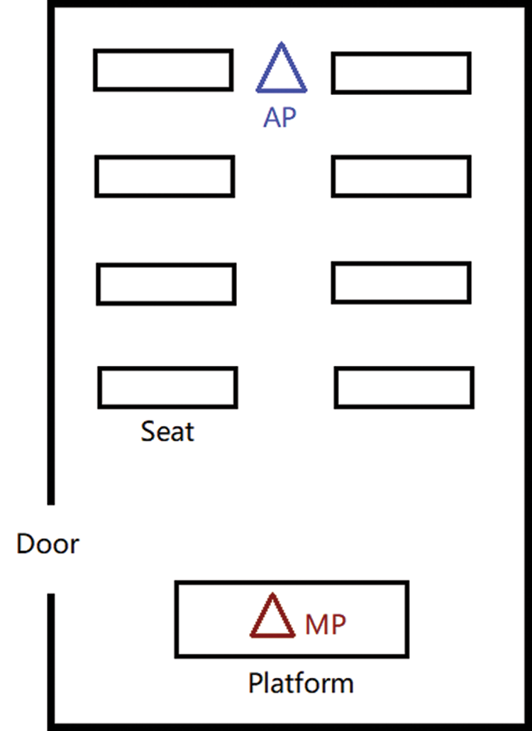
Figure 5: Layout of the experiment environment

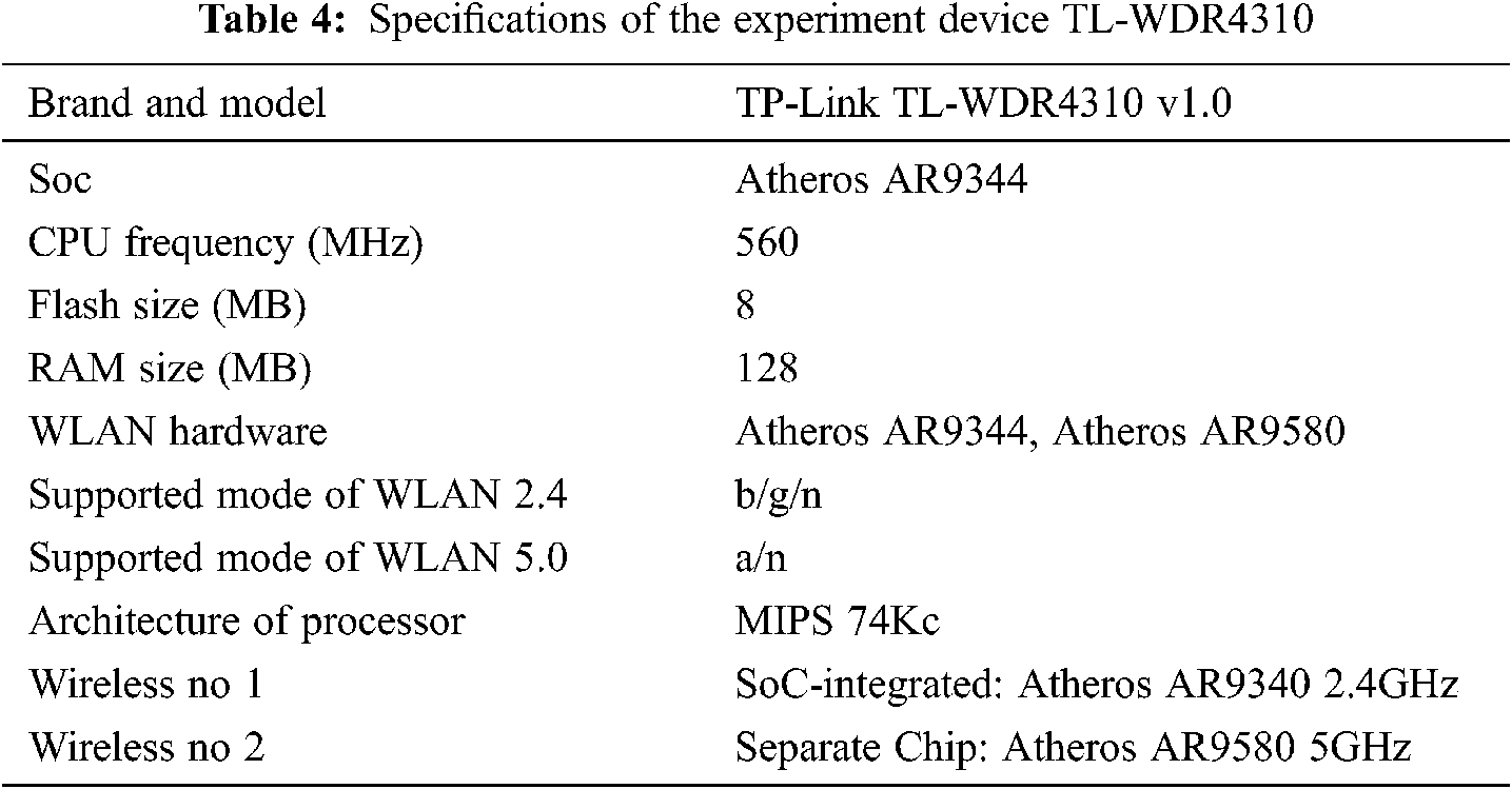
4.2 Specification of the Experiment Device

In this experiment, one TL-WDR4310 wireless router flashed with customized OpenWRT firmware was used to collect CSI data. Tab. 4 displays the specifications of the experiment device.

4.3 Atheros-CSI-Tool

The CSI data was collected using the Atheros-CSI-Tool which is an open source 802.11n measurement and experimentation tool. Based on this tool, detailed PHY wireless communication information was extracted from the Atheros Wi-Fi NICs, including CSI, data rate, the received packet payload, RSSI, etc. All functionalities of Atheros-CSI-Tool are implemented in software without any modification of the firmware. In this experiment, Atheros-CSI-Tool was implemented in the Wi-Fi router with customized OpenWRT firmware.

4.4 Training the ConvNet Classification Model

The ConvNet is implemented using MATLAB Deep Learning Toolbox. Fig. 6 is the graph of training progress.

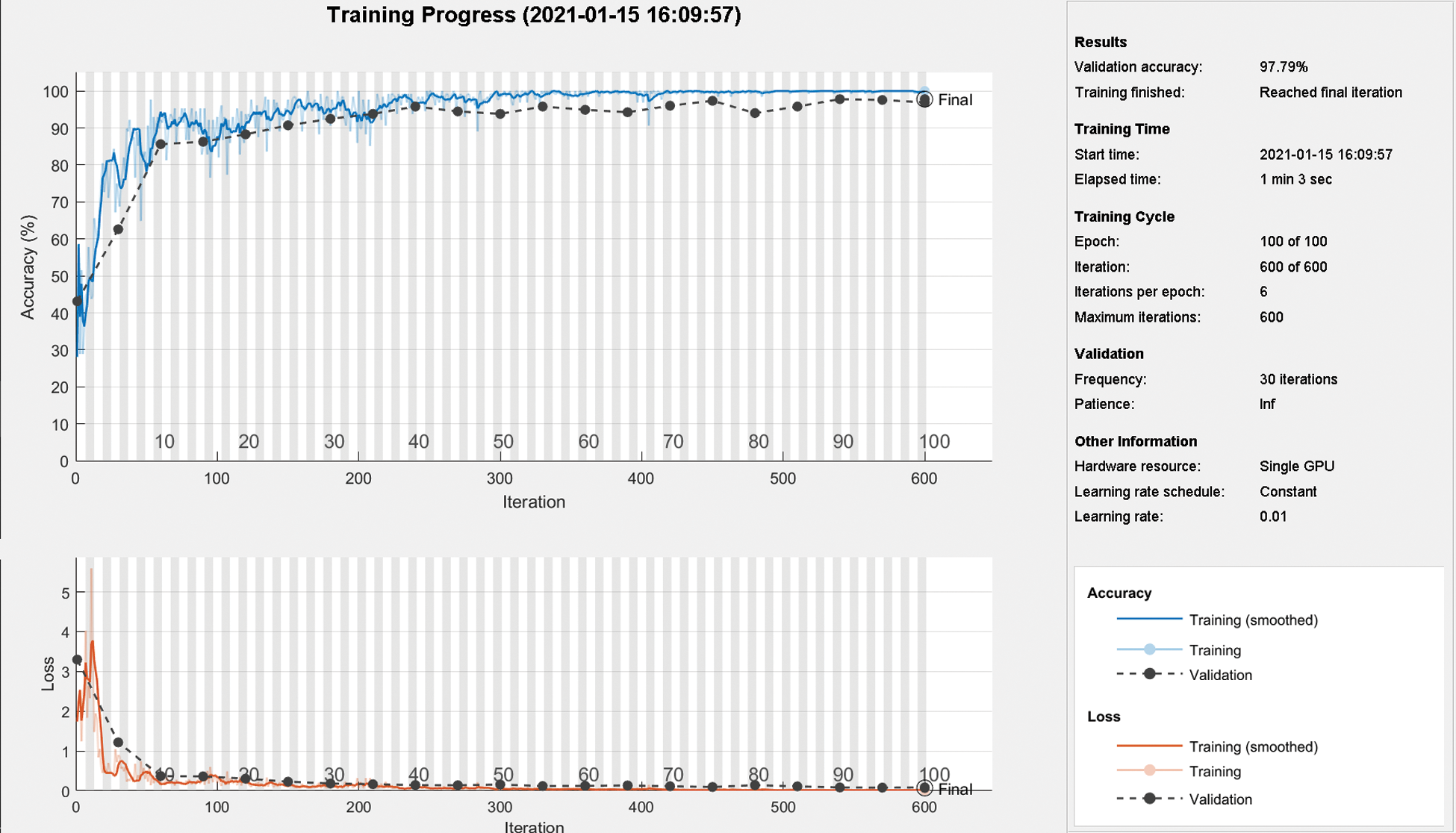
Figure 6: Training progress of the ConvNet with 100 epochs

4.5 Evaluation

Fig. 7 is the algorithm for estimating crowd count.

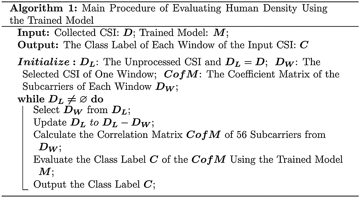
Figure 7: Algorithm: main procedure of evaluating crowd count using the trained model

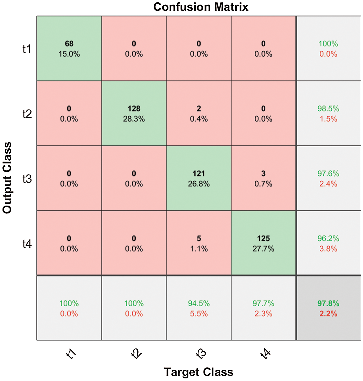
Figure 8: Confusion matrix of the prediction accuracy

The confusion matrix of the evaluation is shown in Fig. 8. It can be seen that the model shows a perfect accuracy when recognizing in Classes 1 and 2 and makes minimal mistakes when distinguishing Class 3 with Class 4. The overall accuracy in all four classes is 97.8%, while the accuracy of recognizing in Classes 1 and 2 is 100% and the accuracy of recognizing in Classes 3 and 4 is 94.5% and 97.7% respectively.

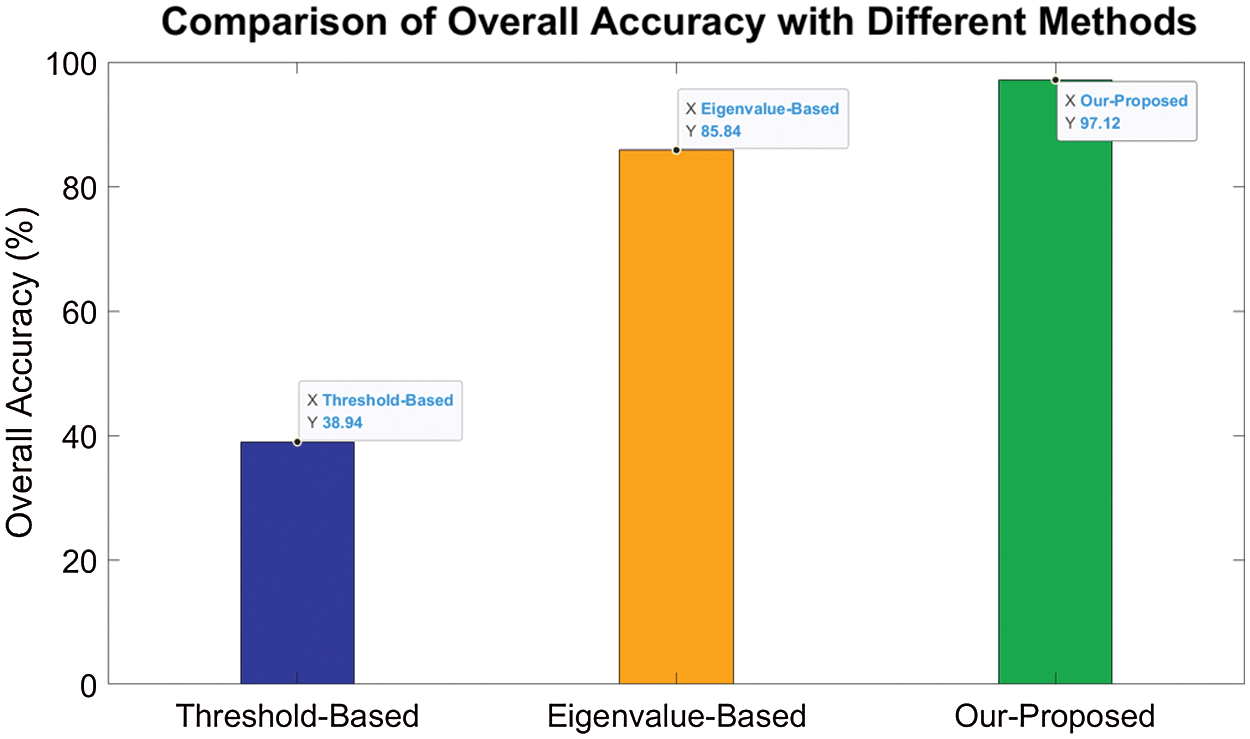
Figure 9: Comparison of overall accuracy with different methods

Two different methods are compared with our proposed method. The comparison bar graph of overall accuracy is shown in Fig. 9. The Threshold-based methods utilize statistical property of the amplitude of CSI, such as variance and mean to recognize the number of people. The Eigenvalue-based methods extract the first several maximum eigenvalues of the correlation matrix of subcarriers. Support Vector Machine implemented with LIBSVM is used to train and evaluate the two methods above [27].

Fig. 10 shows the accuracy of recognizing each class with different methods. It is observed that Threshold-based method almost fails when deployed into different environments except for Scenario 3. The Eigenvalue-based method still shows relatively high performance but the accuracy of recognizing each scenario is lower than our proposed method.

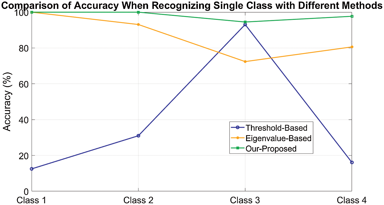
Figure 10: Comparison of accuracy when recognizing single class with different methods

5  Conclusion

In this paper, we presented the design, implementation, and evaluation of a novel lightweight and adaptive passive crowd counting method based on ConvNet. The system addresses the challenges found in the literature such as lack of robustness, low generalization ability, and high computational cost. The main idea is to generate images with fairly low resolution from the correlation coefficient matrix and classify the small images with a relative shallow ConvNet. With only one pair of AP and MP deployed, an overall accuracy of 97.79% is achieved when experimenting with the number of people into four levels.

Currently, we are extending the method to estimate the number of people up to 20 with multiple APs and MPs deployed in public areas.

Funding Statement: This work was supported by the National Natural Science Foundation of China (Grant No. 61802196, url: http://www.nsfc.gov.cn/); Jiangsu Provincial Government Scholarship for Studying Abroad; The Priority Academic Program Development of Jiangsu Higher Education Institutions (PAPD); NUIST Students’ Platform for Innovation and Entrepreneurship Training Program (Grant No. 202010300080Y, url: http://sjjx.nuist.edu.cn:81/CXCY/NUIST/).

Conflicts of Interest: The authors declare that they have no conflicts of interest to report regarding the present study.

This work is licensed under a Creative Commons Attribution 4.0 International License, which permits unrestricted use, distribution, and reproduction in any medium, provided the original work is properly cited.