DOI:10.32604/csse.2022.019987
| Computer Systems Science & Engineering DOI:10.32604/csse.2022.019987 | |
| Article |
On Mixed Model for Improvement in Stock Price Forecasting
1Hunan Vocational College of Science and Technology, Changsha, China
2Hunan University of Finance and Economics, Changsha, China
3Xiangtan University, Xiangtan, China
4University Malaysia Sabah, Kota Kinabalu, Malaysia
*Corresponding Author: Liang Dai. Email: dailiang@hufe.edu.cn
Received: 04 May 2021; Accepted: 08 June 2021
Abstract: Stock market trading is an activity in which investors need fast and accurate information to make effective decisions. But the fact is that forecasting stock prices by using various models has been suffering from low accuracy, slow convergence, and complex parameters. This study aims to employ a mixed model to improve the accuracy of stock price prediction. We present how to use a random walk based on jump-diffusion, to obtain stock predictions with a good-fitting degree by adjusting different parameters. Aimed at getting better parameters and then using the time series model to predict the data, we employed the time series model to smooth the sequence utilizing logarithm and difference, which successfully resulted in drawing the auto-correlation figure and partial the auto-correlation figure. According to the comparative analysis, which focuses on checking the mean absolute error, including root mean square error and R square evaluation index, we have drawn a clear conclusion that our mixed model prediction effect is relatively good. In the context of Chinese stocks, the hybrid random walk model is very suitable for predicting stocks. It can “interpret” the randomness of stocks very well, and it also has an unparalleled prediction effect compared with other models. Based on the time series model’s application in this paper, the above-mentioned series is more suitable for predicting trends.
Keywords: Random walk model; time series model; stock forecasting
With the continuous development of China’s economy, the stock market is booming. During more than 400 years in which stocks have existed, stock forecasting methods have been evolving. Accurate prediction of stock price and avoidance of investment risks are the decisive factors for investors to obtain returns. Although, a related news of significant importance affects odds of probability. This paper focuses on stock forecasting to help investors improve the quality and efficiency of decision-making. In the financial securities industry, stock exists as a form of securities in the financial market; it has strong profitability and liquidity and has a certain degree of risk. It is often said that “if there is an investment, there will be a return,” but it is not applicable in the stock market. “If you do not pay, there will be no return” should be the driving force behind the continuous struggle of most shareholders in the stock market. The changes in the stock market can only be described as unpredictable.
Many factors affect the stock market changes, such as the operating conditions of the company, macroeconomics and policies, the psychology and public opinion of investors, among which the stock price is the most relevant one. The fluctuations in the price of the stock are a repercussion to ‘shocks’ and to the investors. Since the Science and Technology Innovation Board was listed in July 2019, some organizations have predicted that new shares will increase by up to 53 percent on the first day. The natural average increase is 140 percent or more, which shows the randomness and unpredictability of stock price movements. Accurate prediction of stock prices and trends has become an fundamental goal of most scholars and experts. This study’s focus is to use the method suitable for the financial market to predict the stock market and that the random walk model can well describe and explain the stock market phenomenon. According to the geometric Brownian motion, the past history of a stock price is fully reflected in present prices.
As early as 1900, Bastille had affirmed that the price change of commodities showed a random walk model, all of which indicated that randomness was everlasting. The random walk model has features of simplicity and remarkable prediction accuracy, and it is widely used in finance, biochemistry, and other industries. The realization of accurate stock forecasting can give people a relatively reliable investment direction, increase market liquidity, and bring immediate benefits to people. The study of random walk theory can be traced back to 1900. Louis Bachelier once affirmed that commodity price changes are accidental, while market transactions follow the principle of “fairness”. He put forward for the first time the idea that market returns are subject to an independent and uniform distribution, but no further empirical research has been done on this hypothesis. In the following decades, this theory was developing very quickly. Osborne (1964) made clear that stock prices had the characteristics of “random walks”. Fama (1965) concluded that the stock market is as efficient as a whole. Fama (1965) drew the following conclusion in his doctoral thesis: “it can be said that this article uses a large number of strong evidence to prove that the average return on the random stock investment is higher than that of other investments-random walk theory, and then forms the efficient market hypothesis.” The exploration of random walk theory was also going deep. For example, Merton (1980) proved that stock price variance could be known from its early clash. Stock price forecasting has always been a research topic for many experts and scholars in finance, who use different methods to predict stocks [1,2]. Zhong Xuhui comprehensively analyzed the stock forum’s emotional information and established a new mathematical model combined with time series to predict the stock trend [3]. Deng Guishi constructed a feedback random walk model. The main factors that affect the stock price can be determined, and the parameters need to be improved in terms of parameter optimization [4]. Kang Jianwei used the Grey model to predict SNP stocks accurately, but he found that the Grey prediction model was not suitable for stock price prediction with a rapid change of rising and falling rhythm [5]. Sun Boyuan put forward that the LSTM neural network model is the optimal model to predict stock price change in the future. He also combined the LSTM algorithm with linear algebra to optimize the forecasting stock system model. But the model is based on the calculation of big extreme data and human and material resources, and there can be no error [6]. Chen Xiaoling used the ARIMA model and BP neural model to predict the stock and considered that both of them could predict effectively but did not form a complete investment decision [7]. Liu Haiyue established the AR model, RBF, and GRNN neural model based on MATLAB software, and made a rolling prediction of stock. It is considered that the AR model was unstable, and the GRNN prediction effect was better than the RBF model [8]. Hong Jiahao and so on used artificial neural networks and random walk combination models to predict exchange rates, improving the overall prediction accuracy [9]. Combining the time series model and the support vector model, Tang Xiangyan and others constructed a hybrid model, and the producer price index is measured accurately [10]. Most of the studies are based on the assumption that stocks have certain laws but briefly ignore financial data’s randomness. At the same time, these studies also rely heavily on past sample data. They need a large number of sample data to achieve accurate prediction, and some methods can not be applied to all stock forecasting.There are some limitations. In this paper, the stock is predicted based on the random walk model. According to the Markov characteristic of the stochastic process [11,12], tomorrow’s process value depends only on today’s process state.It does not depend on any other “historical” state or even on the whole path of history. The stock price is not only the focus of investors but also the focus of managers and economists. The ultimate goal for forecasting stocks is to provide investors with better investment advice and a better economic environment for society and the country.
To predict the stock better, this paper uses comparative analysis to indicate a specific stock. Under the premise of predicting the stock by a random walk model, the time series model is added to denote the stock, and finally, the prediction results are compared. Through a large number of literature reviews [13–17], we knew that the short-term stock forecasting effect of the time series model is good, so how about the random walk model’s impact on the short-term stock price prediction? For the fluctuation of the stock price, referring to the law of garlic price fluctuation under the same market conditions, a Garch model is constructed to analyze the price fluctuation of garlic, so we can also try to construct the fluctuation model to analyze the law of stock price fluctuation [18]. In this paper, the author employed the jump-diffusion model based on geometric Brownian motion to predict the stock data of HTHT in the recent ten years. The model predicts the stock price on the second day based on the current time’s stock price. After drift, random normal, Poisson distribution and random jump, a large number of random sequences have been produced, and a lot of tests have been carried out.
After the parameters with a excellent fitting effect are determined, the next day’s stock price is predicted. The predicted stock price is used to repeat the operation and get the next day’s stock price. Finally, the stock price for the next ten days can be obtained. And by comparing it with the actual stock price, the prediction accuracy can be concluded. Based on the time series model’s stock price prediction, the stability of weekly data is tested. It is an unstable series. Making it stable by logarithmic, moving average and difference processing, and the auto-correlation diagram and partial auto-correlation diagram are drawn. By determining the appropriate parameters, the stock data for 2019 is predicted. Finally, according to the two’s comparative analysis, including checking the mean absolute error, root mean square error and R square evaluation index [19], the research concluded. The framework of this research is as follows: the first part is to introduce the current situation and significance of stock forecasting; The second part is to analyze and explain the principle and the related theory of the two models; The third part is to use the two models to fit and analyze the actual data, and in the process of the experiment to optimize the parameters of the model; the fourth part is to analyze the results of the role, and draw the conclusion.
Random walk theory is also called random walk [20]. Random walk theory holds that the change in the stock price in each period is random and unpredictable. Generally speaking, the probability that tomorrow’s share price may be higher than today’s share price is the same as it may be lower. Therefore, the best forecast for tomorrow’s share price in today’s share price uses the current stock price to predict the next day’s stock price. The core of random walk can be well expressed by Eq. (1), in which t is used to represent the current time, St is used to describe the closing price of the present time, and St−1 is used to represent the error term, while the success of a random walk model depends to a large extent on the random error term.
The formula represents the assumption that the stock price of t time is different from the stock price of t times, and there is an error term between them. The error term has the characteristics of zero mean value and fixed variance. With the increase in the number of measurements, the positive and negative errors can be compensated against each other.The average value of the error will gradually tend to become zero. According to the random walk hypothesis, the stock price change in the stock market is like a drunk’s behaviour, which is irregular. If the long-term trend factor is taken into account, the random walk model described in Eq. (2) can add a drift term, the trend term, a drift term. It can be written as follows:
So the prediction error increases with time, and the confidence intervals predicted by the two random walk models are shown in the Figs. 1 and 2.
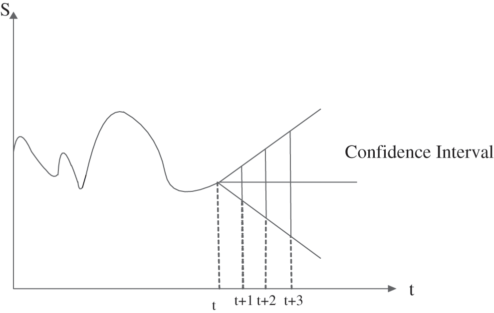
Figure 1: Prediction confidence interval diagram of random walking model
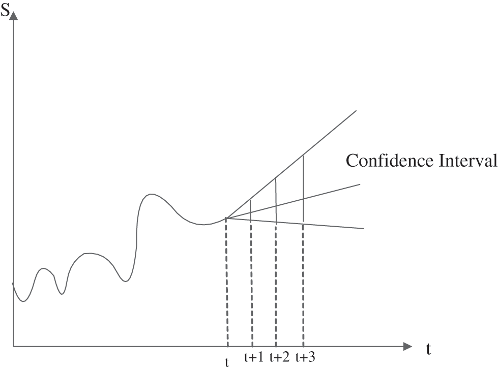
Figure 2: Prediction confidence interval diagram of the random walk model with drift term
The random walk model’s prediction error’s confidence interval with a drift term is smaller and more accurate. Based on the random walking model’s accuracy of stock prediction, a random walking model based on Geometric Brownian Motion(BM)is used. The geometric Brownian motion model has two parameter drift terms and diffusion(fluctuations), which are very similar to the random walk through model structure with a drift term.In contrast the jump-diffusion model is based on the diffusion model of standard geometric Brownian motion (GBM) [21]. The prediction formula of geometric Browan motion after Euler dispersion is Eq. (3).
Until 1976, Meron released his jump-diffusion model to better simulate stochastic processes by adding jump terms to the geometric Brownian motion [22], which are included in Eq. (4).
The meaning of each parameter in the above formula is as follows:
St represents the stock price of t time, Zt is the standard Brownian motion random variable, Δt is a fixed discrete time interval, r denotes a constant risk-free short-term interest rate, and Jt represents a jump indicating a distribution of t days. σ represents the ongoing volatility, yt represents Poisson distribution with density λ and rJ represents the jump drift correction to maintain the risk neutrality.
Time series [23] analysis is based on the time series data observed by the system. The theory and method of the mathematical model are established by curve fitting and parameter estimation. It is generally carried out by curve fitting and parameter estimation (such as the nonlinear least square method). Time series analysis is commonly used in national economic macro-control, regional comprehensive development planning, enterprise management, market potential prediction, meteorological prediction, horological prediction, earthquake precursor prediction, crop disease and insect disaster prediction, environmental pollution control, ecological balance, astronomy and oceanography.
We are surrounded by patterns that can be seen everywhere.People can notice the relationship between the four seasons and the weather, the rush hour model in terms of traffic volume, your heartbeat or the sales cycle of the stock market and specific products. Analyzing time-series data is very useful for discovering these patterns and predicting the future.
2.2.2 Common Time Series Model
(i) Auto-regression model(AR)
The Auto-regression model uses observations from previous time steps as input to a regression equation to predict the value at the next time step. Such as predicting x current time by using the information {X1,X2,…,Xt−1} before the same variable x under the assumption that x and are linear. The formula can be expressed as follows:
where
(ii) Moving Average Model (MA)
Moving average model, also known as moving average process, is a common method to model unstable time series. It points out that the output variable is linearly dependent on the current value and the past value of different random terms. It is defined as Eq. (6).
(iii) Auto-regressive moving average model (ARMA)
The auto-regression moving average model can be regarded as a weakly stationary stochastic process composed of auto-regression model and moving average model. When the system is a series of unobserved shocks (the MA part) and a function of its behavior, it is appropriate to use ARMA. For example, stock prices may be impacted by basic information, as well as technology trends and mean regression effects. ARMA (p, q) represents p-order AR and q-order MA, which are defined as Eq. (7):
(iv) Auto-regressive integrated moving average model (ARIMA)
In the analysis of statistics, economics and time series, the ARIMA model is an extension of the ARMA model, both of which are suitable for the timing data to better understand the future points in the data and the prediction sequence. ARIMA can be used in the case of data non-steady state. An ARIMA (p, d, q), AR is a"self-regression”, p is the number of auto-regressive items, MA is a “sliding average”, q is the number of sliding average items and d is the number of difference (order) to make it a stable sequence, where L is a time lag operator. d ∈ Z, d > 0. It is defined as Eq. (8):
The stock data were sourced from Yahoo Finance net. This research used the stock price data of Aerospace Macro from 2010 to 2019. The primary data, as shown in Fig. 3, mainly include the highest price, the lowest price, the closing price, the opening price, the trading volume of the day and the closing price of the previous restoration right, with a total of 2379 lines of data.
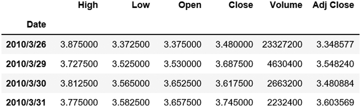
Figure 3: Initial data
Because the collected data are more complete, no further cleaning is required. In this study, the closing price is mainly used, and the closing price is representative to a certain extent.
Due to the large amount of data obtained, the data were sampled every week for better prediction, and the mean value of each week was taken for frequency reduction processing.
The random walk model mainly uses the jump-diffusion model to predict the last 10 data, and the time series model uses the data from 2010 to 2018 to predict the 2019 data.
In this study, we randomly selected HTHT stock as the research data.We obtained the stock data from March 26, 2010 to September 9, 2019, including the highest price, the lowest price, the opening price, the closing price and the 5-day average value, among which most scholars used the closing price to calculate the rate of return and forecast the stock price, because the closing price was representative to a certain extent. The closing price often reflects the attention of market funds to stock and has the function of predicting the deductive direction of the next trading day, so the very first data used to indicate the stock price is mainly the closing price of the stock. The central forecast was the closing price in 2019, and two forecasting methods compare the final prediction results.
3.2.1 Random Walk Model Experiment Process
In the previous model introduction, the random walk model has two forms. It can be seen from Figs. 1 and 2 that the random walk model’s confidence interval with drift term is narrower and the confidence level is higher than that of the zero-drift random walk model. So it is more suitable to choose the random walk model with a drift term. In the stochastic simulation, geometric Brownian motion is the most common stochastic model to simulate the future stock price.To have a better stochastic simulation effect, the jump-diffusion model is adopted.
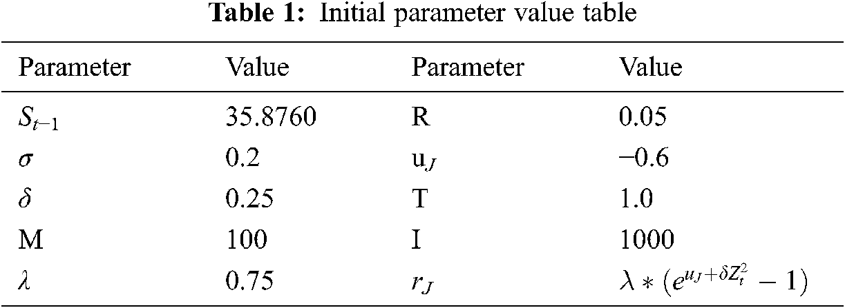
Because there are many parameters of the model, in order to achieve better experimental results, the initial parameters are selected as the reference [24,25]. The parameters of preset stocks are fixed, and the main parameters are adjusted at a later stage.
The research mainly predicts the last ten share prices, the 10-week average from July 1, 2019, to September 9, 2019. According to the corresponding formula, 35.8760 of the stock’s closing price on January 7, 2019, is used to predict the stock price of July 8, 2019, and the parameters are designed as shown in the following Tab. 1:
(i) Exploration of parameter M
What the author got was 1000 line charts with 100 walks. These randomly generated data are a large number of data generated around the initial values. Finally, we need to extract a suitable value from these data, choose a relatively simple average, and try to average the 1000 data of the 10th, 50th and 100th walk, the final results are shown in Fig. 4:
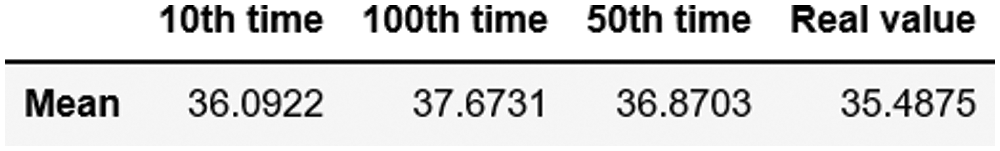
Figure 4: Selection of prediction parameter M
The value of the 10th time is close to the actual value, so the average value of the 10th time is selected as the official forecast value, that is, the value of July 8, 2019. For predicting the value of the next cycle, the value of July 8, 2019, is used as the initial value, and then the value of the following Monday is predicted.
(ii) Exploration of parameter I
The characteristic of the stochastic process is that all the data sets that may be realized are obtained by a large number of data calculation, which needs to be simulated constantly. So the simulation times are divided into 1000 times, 5000 times and 10000 times, and the average values of 1000, 5000 and 10000 times data during the 10th walk are also used to predict the last 10 stock data. And the final prediction data are obtained. In the end, the error coefficient and accuracy are obtained from the predicted data. The test results are as Fig. 5.
(iii) Exploration of parameter λ
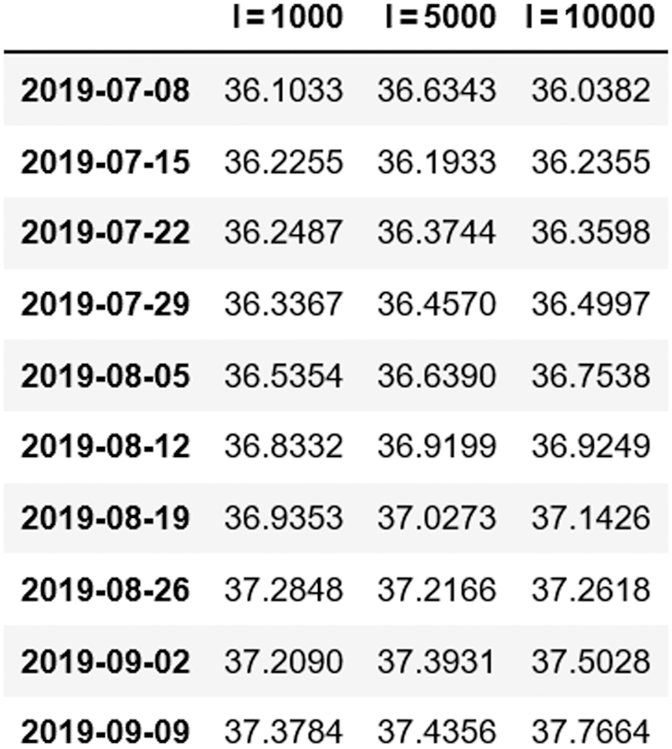
Figure 5: Selection of prediction parameter I
After the exploration and estimation of the parameters M and I, the jump density coefficient λ is explored. The parameter mainly involves the selection of jump degree λ = 0.75 and λ = 0.3, which represent high density and low density, respectively. The two jump-diffusion paths are as Fig. 6.
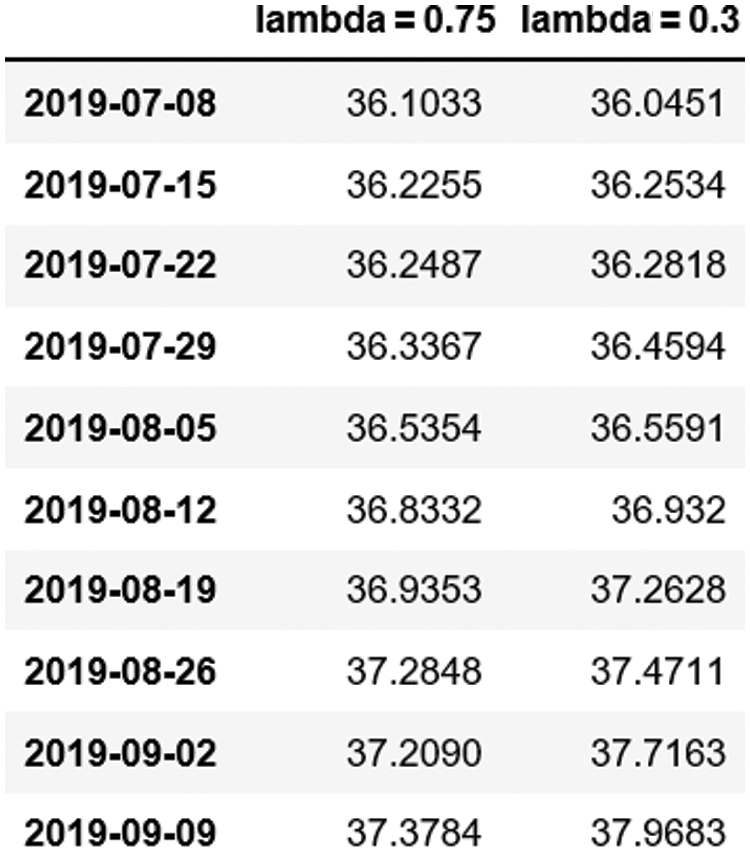
Figure 6: Selection of prediction parameter λ
For different jump density selection, the final result is not the same.
3.2.2 Common Time Series Model
The Time series prediction method is an extended prediction method for the current situation based on historical data, mainly including auto-regressive model, moving average model, auto-regressive moving average model and regression comprehensive moving average model, etc. This study adopted the regression complete moving average model for this prediction.
The weekly stock data of the PIESAT from 2010 to 2018 are used to predict the data of 2019. Firstly, the data are visualized and divided into the training set and test set.
Dickey-Fuller is used to test whether the event sequence is stable or not. If it is not stable and has a noticeable trend, the line is eliminated and processed by logarithm and moving average. The effect is as shown in Fig. 7. Then the obtained data is calculated by d-order difference. It can be seen from Fig. 8 that the second-order difference is better than the first-order difference. Into a stationary time series???. In the initial test results, Test Statistic = 1.449729 is more significant than each test value.That is, it is an unstable sequence. After stabilization treatment, the critical importance of Test Statistic = −11.79445 is less than 1%.
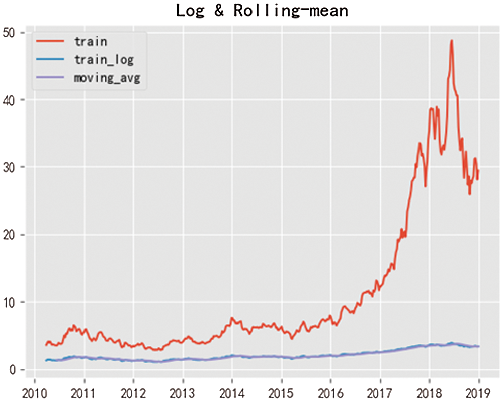
Figure 7: Eliminate trend processing
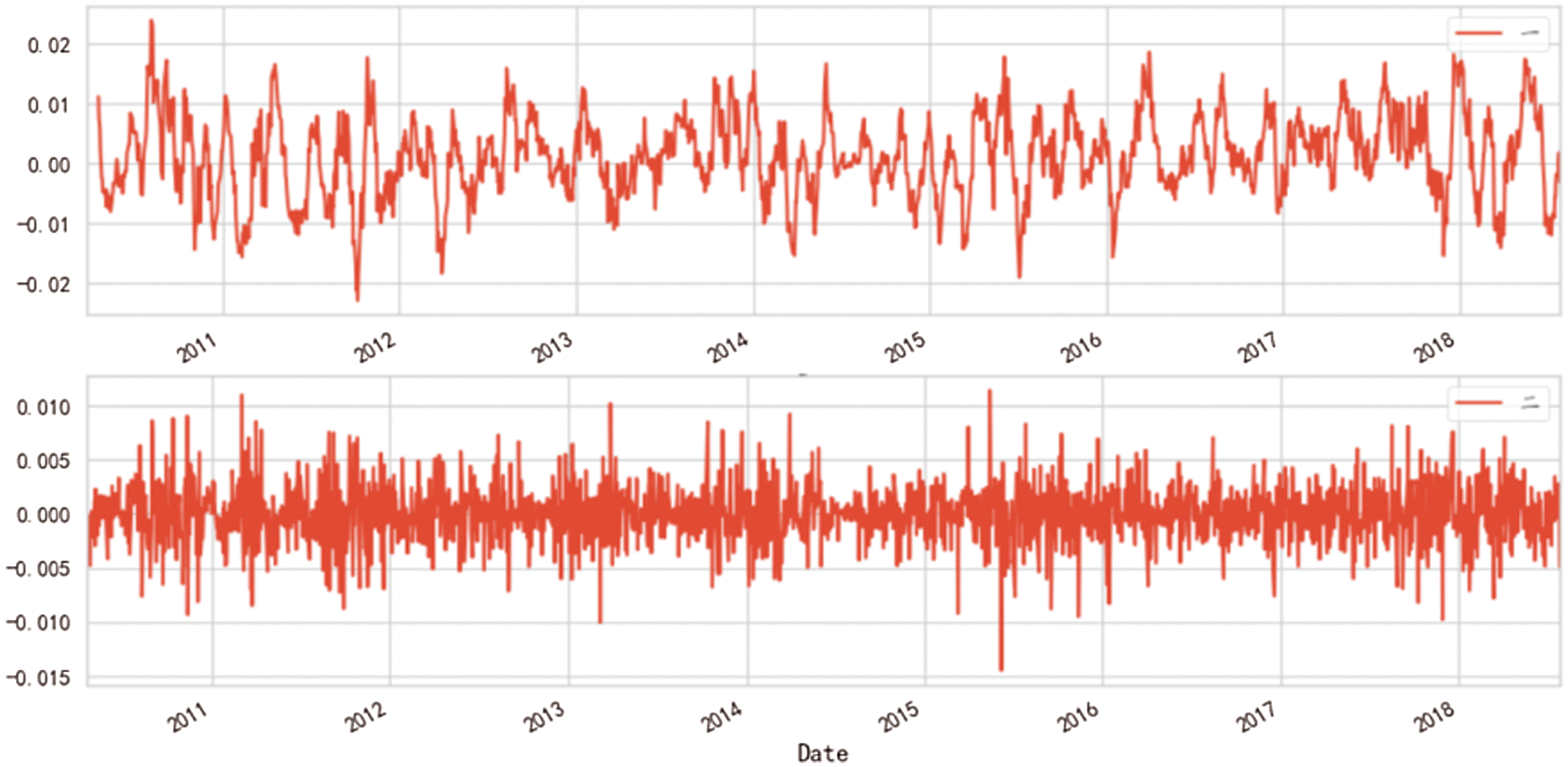
Figure 8: Differential effect diagram
After the stationary time series is obtained, the auto-correlation coefficient ACF and the partial auto-correlation coefficient PACF of the stationary time series are obtained by observing and analyzing the auto-correlation graph and the partial autocorrelation graph, as is shown in Fig. 9, and the best class p and order q is obtained. From the above d, q, p, the ARIMA model is obtained, and then the model is tested. It can be seen from the graph that after the first order in the confidence interval, the following values tend to be 0, so let p = 1, q = 1.
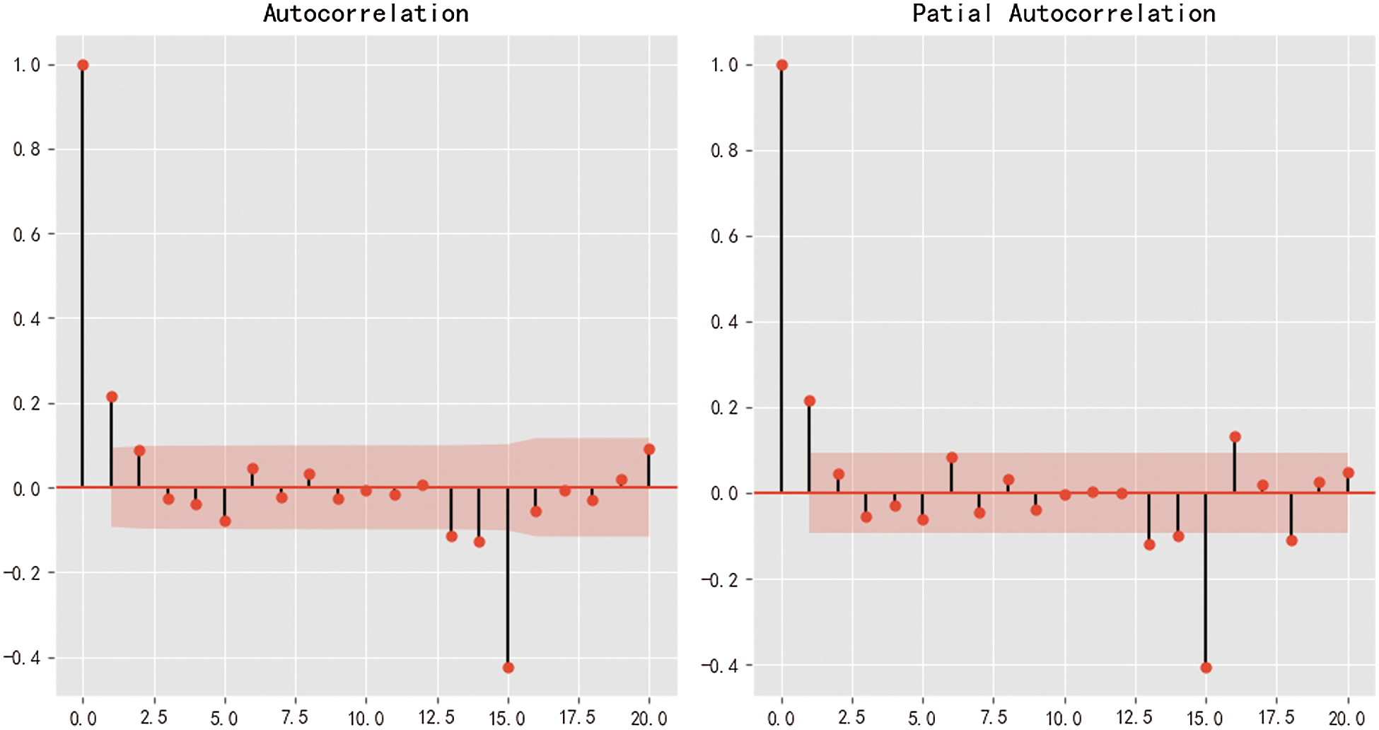
Figure 9: Auto-correlation graph and partial auto-correlation graph
Finally, the prediction results are compared with the test data, and the mean square error and accuracy are calculated. The results are shown in the fourth part.
4.1 Results of Random Walk Model
Through the random prediction of the stock price from July 8 to September 9, 2019, the parameters in the model are adjusted to achieve a relatively good prediction effect [26] .
It can be found that the error is the smallest and the prediction accuracy is the highest when the parameter M is 10, the number of iterations I is 1000 and the jump density is 0.75 from Fig. 10.
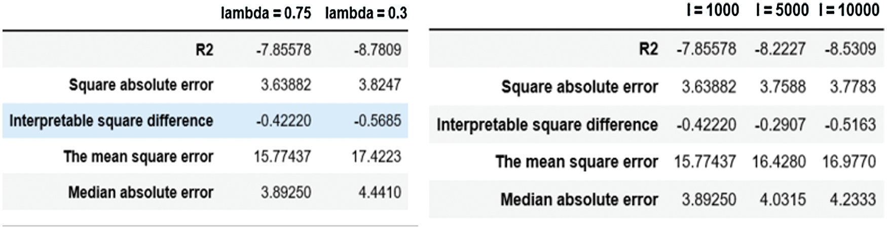
Figure 10: Error result comparison diagram
Diagram: In this experiment, the mean absolute error (MAE), mean square error (MSE), a fundamental median mistake is mainly adopted, which can explain the error evaluation indexes such as variance and R2 fit indicator, in which the optimal value of the first three is 0. The optimal value of the latter two is 1. The closer the optimal value is, the more accurate the prediction result is.
As for different jump densities, the slower it increases, the closer to the actual value, while the larger it grows, the larger the error. In Fig. 12, the difference of absolute square error between the two is slight, and the contrast of absolute median mistake is significant, indicating that the jump density between the two is largely deviates from the median. In this example, it is more suitable for the high jump density, and at the same time, it can be verified that the stock jump density is more significant.
From Figs. 11 and 12, with the increase of the simulation path, from 1000 to 5000 times, and then to 10000 times, the predicted broken line slowly tends to flatten, which is closer to the stock price chart in reality, and the simulation path is less. From the test data, we can also see that the error is more minor when it is equal to 1000. The experimental results show that there are different methods suitable for various research problems. Most people believe that the more times of simulation, the better. Actually, it is not so.
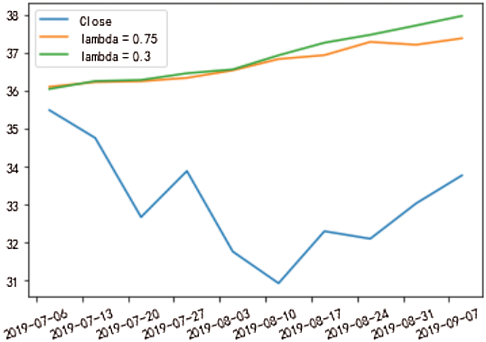
Figure 11: Prediction result diagram of different jump density
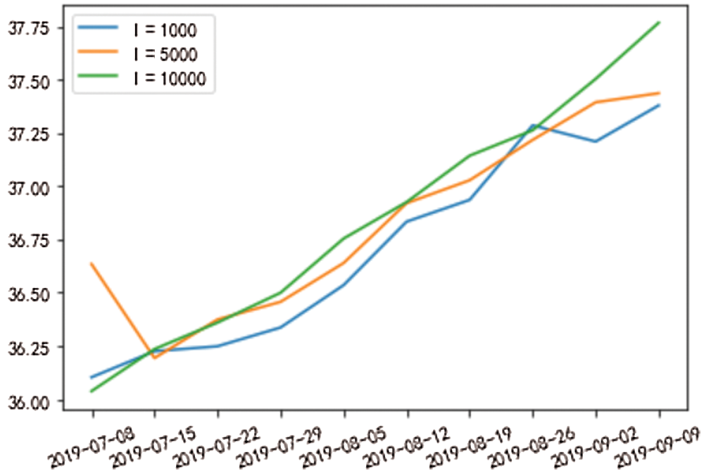
Figure 12: Prediction results of different simulation times
In this experiment, only the important and obvious parameters are adjusted and compared.The model parameters with relatively small errors are selected.The stock is predicted, and more research and exploration can be made [27]. The random walk theory is a reliable random model based on the jump -diffusion model and a lot of theoretical basis. It can be applied to different research direction, dependent on the characteristics of the research object. By choosing an other walking method, researchers can make continuous improvement to calculate its unpredictability side starting from the previous theoretical research results. This study can also be called a quantitative one because of the random walk model with great randomness and uncertainty,.The random walk model is an integration of all possibilities and a challenge for technological forecasting.
4.2 Results of Time Series Model
The time series model is used to predict the stock price. The training set is the stock data from 2010 to 2018, and the test set was the total stock data in 2019. The data shows that the stock has an inevitable upward trend, and the closing price was an unstable sequence from 3.48 RMB in 2010 to 33.7 RMB in 2019.The result is as Fig. 13.
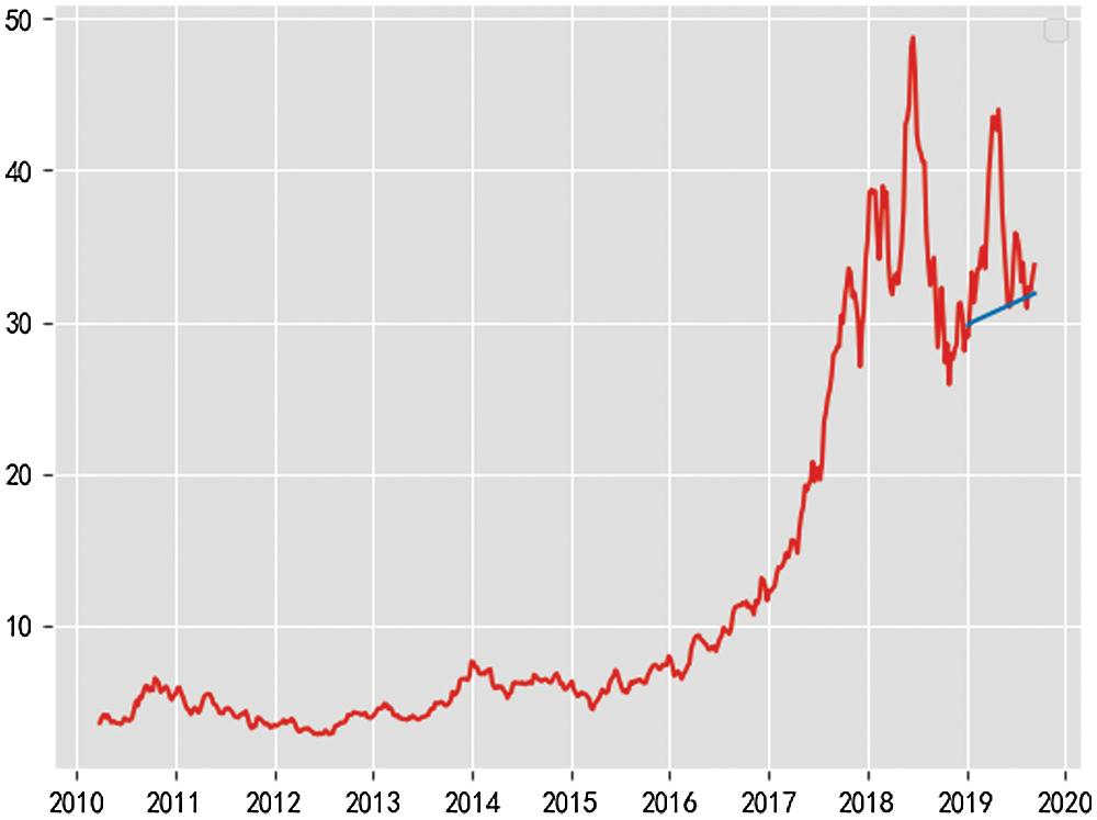
Figure 13: Prediction result chart
After logarithmic, moving average and difference processing, the stationary time series is obtained, and the corresponding parameters in the time series model need to be determined. According to the correlation analysis, the final prediction model is p = 1, d = 1, q = 1. The final results are as follows:
The error detection results are as follows:
The mean square error is 33.57760505468555.
Square absolute error is 4.143031196290987.
Median absolute error is 3.1189309574067874 .
Interpretable square difference is:−0.057654573976772205.
R2 is:−1.04763258629333229.
The final fitting effect is not satisfying.The prediction curve showed the lack of inevitable volatility, but probably predicted the upward trend. There may be the following reasons:
There is no apparent seasonal factor for oberving the data, so there is no operation to remove the data’s seasonal element. There may also be some deviation in the selection of model parameters.
Another important reason lies in the selection of samples, and the size of samples is the pieces. The sample size chosen this time is relatively large, but the gap between them is also rather large.The increase is noteiceable.
The time series model is more suitable for predicting the trend.
In this paper, the random walk model and time series model predict the closing price of an aerospace macro stock in 2019. Compared with the two model’s prediction results the prediction results of the random walk model are better than those of the time series model, and the prediction effect is relatively good. The random walk model is very suitable for predicting stocks. It can “interpret” the randomness of stocks very well, and it also has a remarkable prediction effect compared with other models. Based on the time series model’s application in this paper, the series is more suitable for predicting trends.
In this experiment, one of the problems involved in both of them is the selection of parameters. The model parameters have different meanings and functions, so parameter selection is essential, which is also a topic worthy of our further study. The two prediction methods are relatively simple.In view of our limited knowledge and energy, the final prediction effect is not satisfying.There is a lot of room for improvement in solving the optimization problem.
The application of random walk theory to the stock market is not limited to predicting the stock price; it is also suitable for other financial fields. For investors, managers, it is an excellent predictive player. For economic management scholars, it is a data detector containing unlimited possibilities.
Funding Statement: This work was supported by the 2020 Hunan Natural Science Foundation Project “Research on the Key Technologies of a Personalized Learning Platform for Higher Vocational Students Based on Self-Expanding Knowledge Base and Multimodal Portraits"(2020JJ7041), partly supported by the National Natural Science Foundation of China (No. 72073041).
Conflicts of Interest: The authors declare that they have no conflicts of interest to report regarding the present study.
1. L. Sheng, Q. Ki, W. K. Cong and Z. Wei, “Review on machine learning in stock price forecasting,” Economist, vol. 3, no. 4, pp. 71–73, 2019. [Google Scholar]
2. E. David and N. Mehdiyev, “Stock market prediction using a combination of stepwise regression analysis, differential evolution-based fuzzy clustering, and a fuzzy inference neural network,” Intelligent Automation and Soft Computing, vol. 19, no. 4, pp. 636–648, 2013. [Google Scholar]
3. X. Tang, C. Yang and J. Zhou, “Stock price forecasting by combining news mining and time series analysis,” in 2009 IEEE/WIC/ACM Int. Joint Conf. on Web Intelligence and Intelligent Agent Technology, Milan, Italy, pp. 279–282, 2009. [Google Scholar]
4. D. G. Shi and L. B. Quan, “Feedback-type random walk model and its application in stock investment,” Journal of Dalian University of Technology, vol. 6, no. 1, pp. 140–143, 2004. [Google Scholar]
5. K. J. Wei, “Application of grey model in stock price forecasting–A case study of sinopec,” Hebei Industrial Science and Technology, vol. 30, no. 5, pp. 360–363, 2013. [Google Scholar]
6. S. B. Yuan,“Stock forecasting and research based on neural network model,” Electronic Test, vol. 12, no. 2, pp. 69–70, 2019. [Google Scholar]
7. C. X. Ling, “Stock price forecasting based on ARIMA model and neural network model,”Economic Mathematics, vol. 4, no. 2, pp. 30–34, 2017. [Google Scholar]
8. L. H. Yue and B. Y. Ping, “Analysis of time series model and neural network model in stock forecasting,” Mathematics Practice and Knowledge, vol. 41, no. 4, pp. 14–19, 2016. [Google Scholar]
9. H. J. Hao, L. X. Ying and W. B. Hui, “Exchange rate prediction based on artificial neural network and random walk model,” Economic Mathematics, vol. 1, no. 1, pp. 30–35, 2016. [Google Scholar]
10. T. X. Yan, W. Liang, C. J. Ren, C. Jing and V. S. Sheng, “Forecasting model based on information-granulated GA-sVR and ARIMA for producer price index,” Computers, Materials & Continua, vol. 58, no. 2, pp. 463–491, 2019. [Google Scholar]
11. P. Z. Xing and X. L. Tian, “Markov chain and its application in stock market analysis,” Applied Mathematics, vol. 2, pp. 159–163, 2004. [Google Scholar]
12. Z. X. Wei, L. J. Xuan, Z. Yong and L. Q. Kun, “An optimization model of hadoop cluster performance prediction based on markov process,” Computer Systems Science and Engineering, vol. 31, no. 2, pp. 127–136, 2016. [Google Scholar]
13. M. J. Feng, Z. Xing and F. J. Jie, “Time series prediction of air quality index in shenzhen based on ARIMA model,” Journal of Environmental Hygiene, vol. 55, no. 2, pp. 102–107, 2017. [Google Scholar]
14. Y. Z. Ning, M. J. Feng and Z. Xin, “Time series prediction and analysis of PM2.5 concentration in ShenZhen based on ARIMA model,” Modern Preventive Medicine, vol. 45, no. 2, pp. 220–223, 2018. [Google Scholar]
15. Z. Hossain, A. Q. Samad and Z. Ali, “ARIMA model and forecasting with three types of pulse prices in Bangladesh: A case study,” International Journal of Social Economics, vol. 33, no. 4, pp. 344–353, 2006. [Google Scholar]
16. W. Y. Xia and W. Xin, “Short-term stock price forecasting based on ARIMA model,” Statistics and Decision-Making, vol. 467, no. 23, pp. 83–86, 2016. [Google Scholar]
17. S. H. Jian and D. Xing, “Adaboosting neural network for short-term wind speed forecasting based on seasonal characteristics analysis and lag space estimation,” Computer Modeling in Engineering & Sciences, vol. 144, no. 3, pp. 277–293, 2018. [Google Scholar]
18. G. Feng, L. P. Zeng and Z. Chao, “Research on the law of garlic price based on big data,” Computers, Materials & Continua, vol. 58, no. 3, pp. 795–808, 2019. [Google Scholar]
19. K. Akyol and B. Şen, “Modeling and predicting of news popularity in social media sources,” Computers, Materials & Continua, vol. 61, no. 1, pp. 69–80, 2019. [Google Scholar]
20. I. A. Moosa, “Exchange rate forecasting: Techniques and applications,” Economic Management, vol. 6, no. 1, pp. 109–112, 2004. [Google Scholar]
21. P. Prakash, V. Sangwan and K. Singh, “Transformational approach to analytical value-at-risk for near normal distributions,” Journal of Risk and Financial Management, vol. 14, no. 2, pp. 51–57, 2021. [Google Scholar]
22. T. Q. Ming and H. Ran, “Measurement and analysis of default risk of Chinese listed companies–Application of jump-diffusion model,” Quantitative Economy Technical Economy Research, vol. 10, no. 1, pp. 101–105, 2010. [Google Scholar]
23. S. Zhang, Q. Zhou and M. H. Lin, “Goodness-of-fit test of copula functions for semi-parametric univariate time series models,” Stat Papers, vol. 62, no. 4, pp. 1697–1721, 2020. [Google Scholar]
24. L. F. Qi and G. X. Fei, “Theoretical estimation and monte carlo simulation test of interest rate jump diffusion model,” Journal of Management Engineering, vol. 4, no. 2, pp. 95–99, 2009. [Google Scholar]
25. J. Zhe, “Term structure model and parameter estimation of single factor interest rate in jump diffusion process,” Science Technology and Engineering, vol. 36, no. 1, pp. 176–178, 2011. [Google Scholar]
26. B. Franke and T. Kott, “Parameter estimation for the drift of a time inhomogeneous jump diffusion process,” Statistica Neerlandica, vol. 67, no. 2, pp. 145–148, 2013. [Google Scholar]
27. M. Y. Chao, C. Min and C. Z. Wu, “A jump diffusion model with mean regression for warrant pricing in Chinese stock market,” System Engineering Theory and Practice, vol. 1, no. 2, pp. 16–23, 2010. [Google Scholar]
 | This work is licensed under a Creative Commons Attribution 4.0 International License, which permits unrestricted use, distribution, and reproduction in any medium, provided the original work is properly cited. |