DOI:10.32604/csse.2022.020193
| Computer Systems Science & Engineering DOI:10.32604/csse.2022.020193 | |
| Article |
Algorithms to Calculate the Most Reliable Maximum Flow in Content Delivery Network
1School of Computer Science and Engineering, Southeast University, Nanjing, 211189, China
2State Key Laboratory of Smart Grid Protection and Control, Nanjing, 211106, China
3Nari Group Corporation, Nanjing, 211106, China
4Department of Computing Science, University of Aberdeen, Aberdeen, AB243UE, UK
*Corresponding Author: Keke Ling. Email: 1124907997@qq.com
Received: 13 May 2021; Accepted: 13 August 2021
Abstract: Calculating the most reliable maximum flow (MRMF) from the edge cache node to the requesting node can provide an important reference for selecting the best edge cache node in a content delivery network (CDN). However, SDBA, as the current state-of-the-art MRMF algorithm, is too complex to meet real-time computing needs. This paper proposes a set of MRMF algorithms: NWCD (Negative Weight Community Deletion), SCPDAT (Single-Cycle Preference Deletion Approximation algorithm with Time constraint) and SCPDAP (Single-Cycle Preference Deletion Approximation algorithm with Probability constraint). NWCD draws on the “flow-shifting” algorithm of minimum cost and maximum flow, and further defines the concept of negative weight community. This algorithm continuously deletes the negative weight communities, which can increase reliability while keeping the flow constant in the residual graph. It is proven that when all negative weight communities are deleted, the corresponding maximum flow is the MRMF. SCPDAT tries to approach the optimal solution to the greatest extent possible within the limited time, while SCPDAP tries to reach the probability threshold in the shortest amount of time. Both of these adopt the strategy of first deleting single-cycle communities (which contribute more to the reliability with lower time cost). Experiments show that, compared with SDBA, NWCD combined with the probabilistic pruning achieves an order of magnitude improvement in time cost, while SCPDAT and SCPDAP demonstrate better time performance and increased applicability.
Keywords: Content delivery network; uncertain graph; maximum flow; flow reliability
CDN (Content Delivery Network) redirects the user request to the edge cache node that is close to the user. It reduces the content transmission from remote source data nodes; therefore, the user access response time is significantly shortened, and the pressure on the backbone network is effectively reduced [1–3]. As the core of the entire CDN, the load balancing system is responsible for evaluation and scheduling. This system redirects user requests to the most suitable node in the CDN, and as a result, directly determines the entire CDN’s performance [2–5]. The node is often selected from the cache nodes close to the user within a local area to provide content services. At present, this selection generally considers distance, node health, load conditions and supported media formats [6–8]. However, network capacity and flow reliability are not taken into consideration [9–23]. The reason for this is that relevant algorithms such as SDBA have high time complexity, and thus cannot handle the online selection of CDN cache nodes [17–22].
The MRMF belongs to the category of dual-attribute (capacity and reliability) maximum flow problem [17], which can be solved by referring to the “flow-shifting” algorithm of the minimum cost and maximum flow [18–23]. In other words, the problem may be solved using the auxiliary residual graph by deleting the negative weight cycle, which can increase the reliability with the unchanged flow value. Generally speaking, the most suitable CDN cache node can be found among the few candidate edge nodes in a local area that is close to the user. The local area network formed by candidate edge nodes and content request node is relatively simple; that is, there are relatively few nodes and limited number of loops. It is therefore possible to quickly obtain the MRMF using the “flow-shifting” algorithm. However, the segmented relationship between reliability and flow differs from the linear relationship between cost and flow. Therefore, after all negative weight cycles are deleted, there is no certainty that the MRMF can be obtained. In order to solve the problem, this paper defines the concept of negative weight community. Subsequently, it proposes an MRMF algorithm based on the deletion of negative weight communities, termed NWCD (Negative Weight Community Deletion). This algorithm draws on the “flow-shifting” algorithm of the minimum cost and maximum flow, continuously deleting the negative weight communities so as to increase the reliability while also keeping the flow constant in the residual graph. It can be proven that the MRMF is not obtained until all negative weight communities are deleted. Compared with SDBA, NWCD achieves substantial improvements in terms of time complexity. However, due to the high time cost associated with searching for and deleting negative weight communities, the time complexity of NWCD is still large. Thus, NWCD is not suitable for real-time or online applications. Moreover, although multi-cycle communities account for only a small proportion of all negative weight communities, it takes a long time for these to be found and deleted. Therefore, two fast approximation algorithms specifically, SCPDAT (Single-Cycle Preference Deletion Approximation algorithm with Time constraint) and SCPDAP (Single-Cycle Preference Deletion Approximation algorithm with Probability constraint) are proposed to satisfy these real-time applications. SCPDAT and SCPDAP preferentially search for and delete single-cycle communities. Only if no single-cycle community remains, the multi-cycle communities will be searched for and deleted. The former aims to approach the optimal solution to the greatest extent possible within the limited time available. The latter aims to reach the preset probability threshold in the least time possible, and also avoids spending long periods of time on deleting the negative weight communities (with little consequent improvement to reliability). The three algorithms discussed above have their own characteristics and different scopes of application, as well as good complementarity. They can thus meet the needs of different users and can be applied in an actual CDN context.
This paper uses an uncertain graph to model CDN. The candidate edge node is the source point of s, while the content request node is the sink point of t, so that the part of CDN close to the request node can be abstracted into an s-t uncertain graph. The definitions of uncertain graph, uncertain graph s-t flow, reliability of uncertain graph s-t flow and other key concepts are presented in this section to facilitate the description of the problem and related algorithms.
Definition 1. Uncertain graph. An uncertain graph G is a four-tuple G = (V,E,C,P); here, V is the set of vertices in the uncertain graph G, E is the set of edges, C: E → N is the capacity function on the edge, while P: E → (0,1] is the probability function on the edge, indicating the edge’s existence probability. For convenience, the capacity of edge e is denoted as c(e), while the existence probability of edge e is denoted as p(e).
Example 1: Fig. 1 illustrates an uncertain graph. Here, V = {0,1,2,3} is the set of vertices in the uncertain graph, while E = {e01,e02,e12,e13,e23} is the set of edges. Taking edge e12 as an example, the capacity c(e12) on the side is 2, while the probability p(e12) is 0.65.
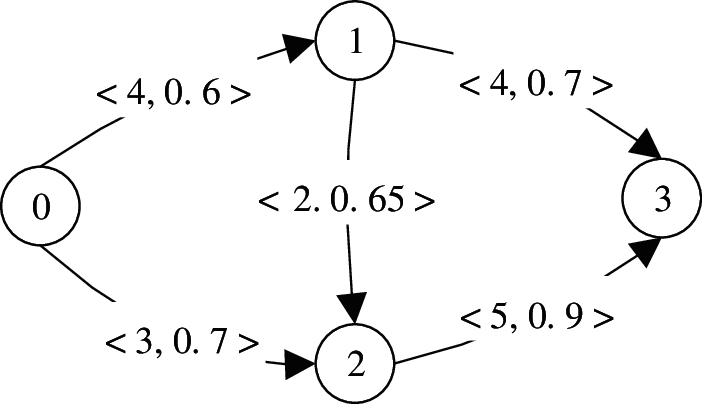
Figure 1: Uncertain Graph
Definition 2. Uncertain graph s-t flow. Given the source point s and sink point t, the s-t flow f in an uncertain graph G is a mapping that maps each edge to a non-negative real number; that is, f: E → R+. Here, f(e) intuitively represents the quantity of flow carried by edge e. A flow f must satisfy the following two properties:
(1) (Capacity conditions) For each edge e ∈ E, 0 ≤ f(e) ≤ c(e);
(2) (Conservation conditions) In addition to s and t, for each vertex v,
Definition 3. Reliability of uncertain graph s-t flow. The reliability of the uncertain graph s-t flow f, R(f), is equal to the product of the existence probabilities of all non-zero flow edges e in the uncertain graph; that is, R(f) =
Definition 4. Uncertain graph maximum flow. Supposing that every edge in the uncertain graph G exists, the maximum flow value fmax that can be transmitted from the source point s to the sink point t is the maximum flow of the uncertain graph G.
Definition 5. Most reliable maximum flow. The most reliable maximum flow is a maximum flow distribution in an uncertain graph, and its reliability is not less than the reliability of any maximum flow distribution in the uncertain graph.
Example 2: Fig. 2 illustrates the maximum flow distribution in the graph in Fig. 1; here, the source point is 0 and the sink point is 3. Suppose that the flow distributions in the three pictures in Fig. 2 are (from left to right) f1, f2, and f3. According to definition 3: R( f1) = 0.6 × 0.7 × 0.65 × 0.65 × 0.7 × 0.9 = 0.17199, R( f2) = 0.6 × 0.7 × 0.7 × 0.9 = 0.2646, R(f3) = 0.6 × 0.7 × 0.65 × 0.7 × 0.9 = 0.17199. The results of these calculations show that the reliability of flow f2 is higher than flow f1 and flow f3, meaning that this flow is the MRMF.
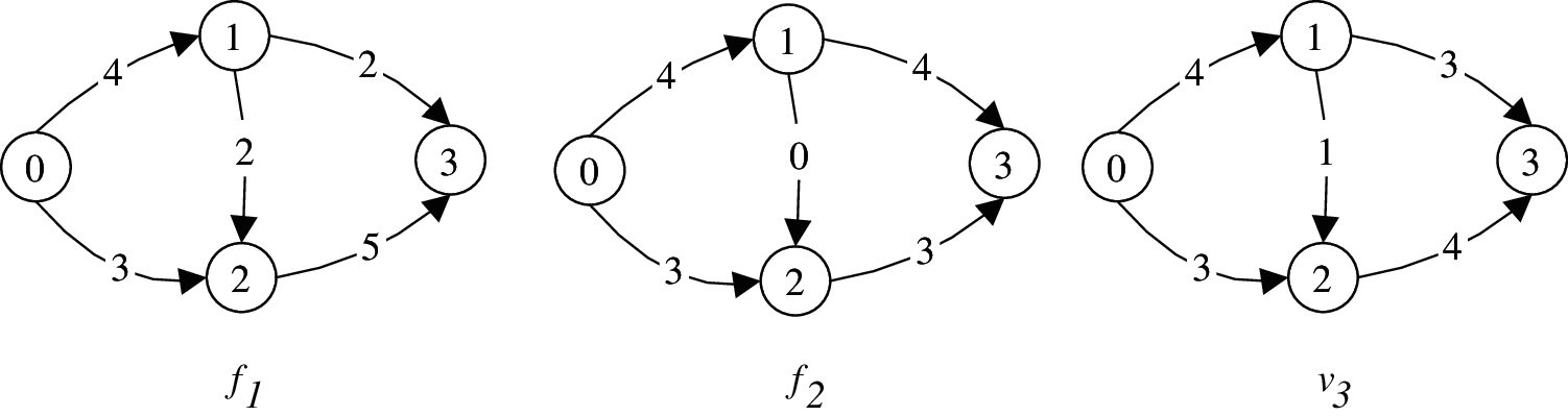
Figure 2: The Maximum Flow Distribution in the Uncertain Graph in Fig. 1
The MRMF problem in the uncertain graph can be defined as follows: the uncertain graph G, the source point s and the sink point t are used to find the MRMF.
Definition 6. Residual graph of uncertain graph. Given an uncertain graph G = (V,E,C,P) and flow f on G, the residual graph Gf is defined as follows:
(1) Gf and G have the same set of vertices;
(2) For the edge eij from i to j in G, there is a forward edge eij in Gf , with a capacity equal to the capacity of eijin G minus the flow of eij. Meanwhile, there is a reverse edge ejifrom j to i in Gf, and its capacity is equal to the flow of eij.
Example 3: Fig. 3 illustrates the residual graph with flow distribution f1 in Fig. 2. Taking edge e13 in the uncertain graph as an example, f(e13) = 2, while c(e13) = 4; because 2 is less than 4, using (2) in Definition 5, the capacities of edges e’13 and e’31 in the residual graph are both 2.
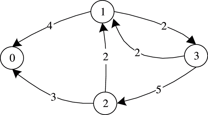
Figure 3: The Residual Graph with Flow Distribution f1 in Fig. 2
Definition 7. Cycle flow cycle_f. The cycle flow cycle_f is a function that maps each edge e’ of the residual graph to a non-negative real number, cycle_f : E → R+. Moreover, cycle_f(e’) intuitively represents the flow carried by edge e’. cycle_f must satisfy the following two properties:
(1) (Capacity conditions) For each edge e ∈ E, 0 ≤ f(e’) ≤ c(e’);
(2) (Conservation conditions) For each vertex v,
Example 4: Fig. 4 presents a cycle flow f’ in the residual graph of Fig. 3. For vertices v1,v2,v3 in the flow, the sum of the flow entering the vertex is equal to the sum of the flow out of the vertex, while the flow on all edges meets the capacity conditions.
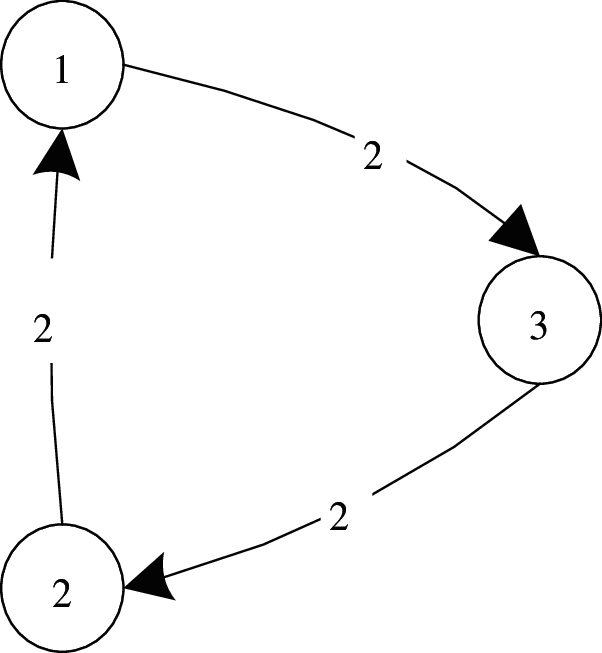
Figure 4: A Cycle Flow f’ in the Residual Graph of Fig. 3
Definition 8. Pre-progress flow (Pre-flow) f’. The pre-flow refers to a cycle flow in the residual graph, which is obtained after progression is supposed to occur in the uncertain graph G.
Definition 9. Weight rule. Let f’(e) be the pre-flow of edge e, where w(e) is the weight value, eij is the forward edge, and eji is the reverse edge. The weight rule is thus defined as follows:
(1) If f(eij) = 0, f’(eij) > 0, then w(eij) = -lnp(eij), w(eji) = 0.
(2) If f(eij) > 0, then w(eij) = 0,
Definition 10. Negative weight cycle. A cycle flow f exists on a cycle structure of the residual graph and is taken as the pre-flow. If the weight of the entire cycle is negative according to the weight rule, the cycle of the residual graph is referred to as a negative weight cycle.
Example 5: Fig. 4 presents a negative weight cycle in the residual graph relative to the cycle flow in the figure. Here, edge e21is the reverse edge, and f’(e21) is equal to f(e12), so its weight lnp(e12) is ln 0.65. Edge e32is also a reverse edge, but f’(e32) is less than f(e23), so its weight is 0. Edge e13 is a forward edge, and f(e13) is more than 0; thus, its weight is 0, and the weight of the entire cycle is ln 0.65, which is less than 0.
There is a key property of the negative weight cycle; that is, after the negative weight cycle is deleted, a more reliable maximum flow distribution will be obtained.
3 The MRMF Algorithm Based on Deleting the Negative Weight Communities
This section focuses on the MRMF problem in the uncertain graph. By drawing on the “flow shifting” algorithm of minimum cost and maximum flow, this section defines the concept of the negative weight community. It subsequently proposes a new MRMF algorithm, NWCD, which is based on deleting the negative weight communities.
For the problem of the dual-attribute (capacity and cost) maximum flow, the minimum cost and maximum flow algorithm involves finding a maximum flow distribution in advance, then moving towards the minimum cost by shifting the maximum flow. The MRMF belongs to the category of dual-attribute (capacity and probability) maximum flow. It is therefore feasible to learn from the minimum cost and maximum flow algorithm and solve the MRMF problem by deleting the negative weight cycle.
However, when considering the problem of minimum cost and maximum flow, the cost function is as follows:
cost(f) = ∑e ∈ E f(e)k(e), where f(e) is the flow value passed on edge e, while k(e) is the cost on edge e. From this function, it can be determined that the cost and flow on each edge are in a linear relationship, and the overall cost is the sum of the costs on each edge. In the MRMF problem, the reliability of the flow is the product of the probabilities of all non-zero flow edges. Although the product can be transformed into the logarithm sum of the probability, it can be observed from the calculation expression that the reliability and the flow value on each edge are in a segmented relationship. When a flow is passing through the edge, provided that it does not exceed the capacity of the edge, its reliability is the edge existence probability p(e), regardless of the flow value. Moreover, this segmented relationship is nonlinear, meaning that the MRMF may not be obtained after deleting all negative weight cycles. For this reason, the present paper extends the concept of the negative weight cycle and defines the concept of a negative weight community.
Definition 11. Negative weight community. A negative weight community is a set of one or more cycles on the residual graph, and at least one edge of each cycle in the set is shared with other cycles. If a cycle flow f exists in the community, f is taken as the pre-flow. According to the weight rule, the weight sum of the entire community is negative.
NWCD is proposed based on the concept of the negative weight community to solve a key problem, specifically that deleting all negative weight cycles cannot guarantee that the MRMF will be obtained. The algorithm first finds any single maximum flow distribution f and constructs its corresponding residual graph Gf; subsequently, it searches for and deletes negative weight communities rather than negative weight cycles in Gf, thereby obtaining a more reliable maximum flow distribution. After deleting a negative weight community, it is necessary to update the maximum flow and the corresponding residual graph, after which the next negative weight community is searched for in the updated residual graph. The above steps are repeated and will continue until there is no remaining negative weight community. At this point, the corresponding maximum flow distribution is the MRMF.
The algorithm implementation (pseudo-code) of the NWCD based on deleting the negative weight communities is presented in Tab. 1.
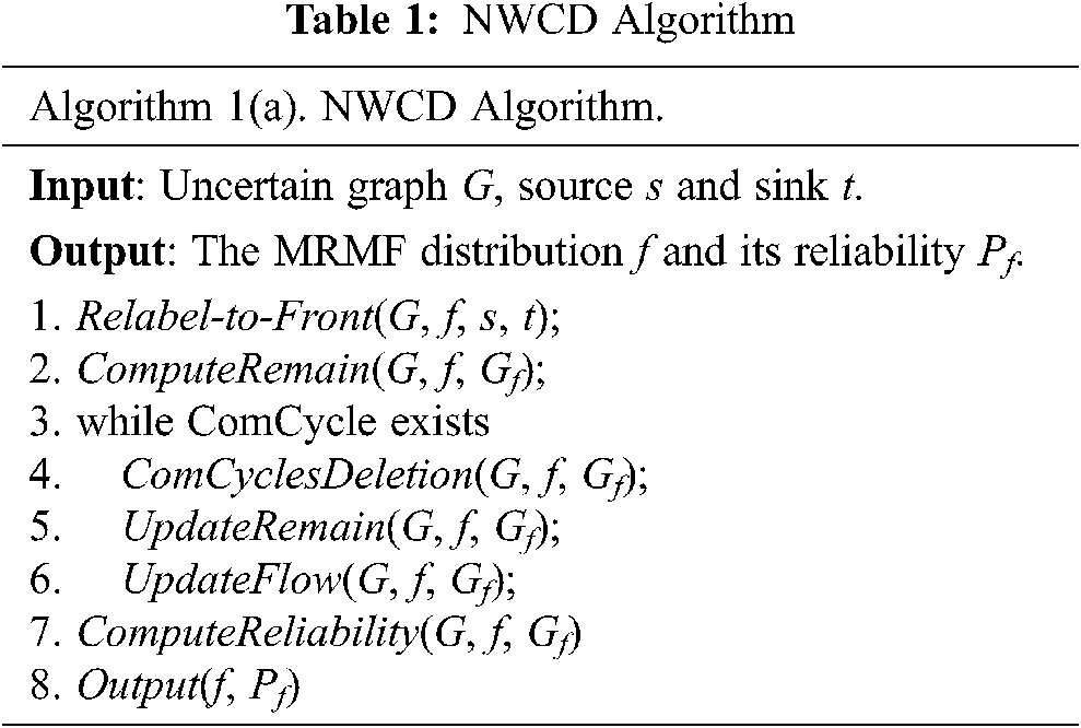
The Relabel-to-Front function uses the relabel-to-front algorithm to find a maximum flow in the uncertain graph G and store it in the vector f. The ComputeRemain function is used to construct the residual graph Gf corresponding to f, after which the function ComCyclesDeletion searches for and deletes negative weight communities in the residual graph Gf. The UpdateRemain function updates the residual graph, and the UpdateFlow function updates the maximum flow distribution. This process will continue until no negative weight community remains. The function ComputeReliability calculates the reliability corresponding to f; finally, the Output function outputs the MRMF and the corresponding reliability.
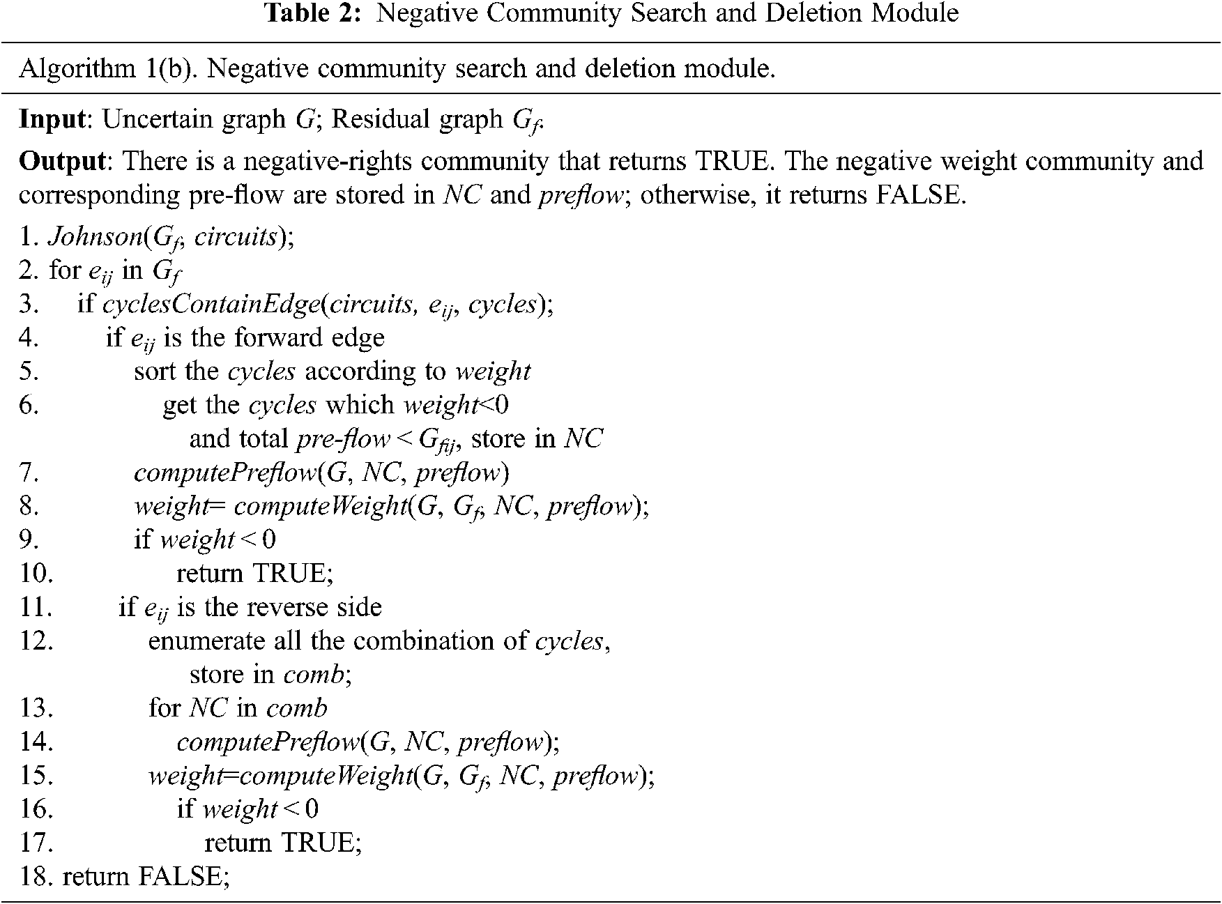
The negative community searching and deleting module, ComCyclesDeletion, is the core of the algorithm implementation. Its basic underlying concepts are as follows:
1) Finding all the cycles in the residual graph using the Johnson algorithm;
2) Enumerating each edge eij in the residual graph. For each edge eij, the module finds all cycles containing the edge eij in the residual graph, then computes the pre-flow f’ that the path Pji can pass when the cycles remove the edge. Subsequently, it calculates the weight of path Pji on the basis of f’;
3) Sorting the cycles according to weight from small to large, if the edge is a forward edge. If a cycle exists that satisfies the conditions, that is, the cycle’s weight is less than 0 and the sum of pre-flow f’ of the path Pji is less than or equal to the capacity of the edge eij, go to 5).
4) If the edge is a reverse edge, all combinations of the cycles that contain the edge are enumerated. If a negative weight community exists in these combinations, go to 5).
5) Saving the negative weight community and its corresponding pre-flow, then returning TRUE.
6) When all edges have been traversed and the function does not return TRUE, the function returns FALSE.
The pseudocode description of the algorithm is presented in Tab. 2.
3.3 Proof of Correctness of the Algorithm
In order to illustrate that the NWCD can ultimately obtain the MRMF, this paper first demonstrates an important property: namely, that removing a negative weight community can obtain a more reliable maximum flow. Based on this property, this paper then proves that if the algorithm terminates, the maximum flow obtained is the most reliable one. Finally, this paper proves that the algorithm can be terminated.
Lemma 1: In the residual graph corresponding to the maximum flow distribution f, if a negative weight community exists and a cycle flow with a maximum flow value of f’ passes through the community, a more reliable flow distribution f1 can be obtained.
Proof: The edge of the negative weight community is considered to be a forward edge or a reverse edge. The definition of the weight rule states that regardless of whether the edge e is a forward edge or a reverse edge, there are two kinds of weights on the edge: specifically, the weight is zero or non-zero. Since an edge with zero weight has no effect on the entire community, only edges with non-zero weight in the negative weight community are considered here.
Suppose that, in the residual graph corresponding to the maximum flow distribution f, there is a community on which a cycle flow with a maximum flow value f’ passes. The weight rule indicates that the weight of the entire community is negative. Further suppose that ei1, ei2, …, eim are forward edges with a non-zero weight in the negative weight community, while ej1, ej2,…, ejn are the reverse edges with non-zero weight in the negative weight community. Thus, the weight of the community W(NC) = w(ei1)+ w(ei2)+…+w(eim)+w(ej1)+w(ej2)+…+w(ejn) = -lnp(ei1)-lnp(ei2)-…-lnp(eim)+lnp(ej1)+lnp(ej2)+…+lnp(ejn). The weight of the entire community is negative, so W(NC) < 0; that is, -lnp(ei1)-lnp(ei2)-…-lnp(eim)+lnp(ej1)+lnp(ej2)+…+lnp(ejn) < 0, then lnp(ej1)+lnp(ej2)+…+lnp(ejn) < lnp(ei1)+lnp(ei2)+…+ lnp(eim). By transforming the inequality, we can obtain p(ej1)*p(ej2)*…*p(ejn)<p(ei1)*p(ei2)*…* p(eim).
From another perspective, by progressing the pre-flow f’ in the negative weight community, the changes in reliability of the maximum flow distribution f1 can be divided into two cases depending on which edge has non-zero weight. If the edge is a forward edge, the reliability of f1 is equal to the reliability of f multiplied by the probability value corresponding to the edge. If the edge is a reverse edge, then the reliability of f1 is equal to the reliability of f divided by the probability value of the forward edge corresponding to the edge. After deleting the negative weight community, the reliability P(f1) = P(f)*(p(ei1)*p(ei2)*…* p(eim))/(p(ej1)*p(ej2)*…*p(ejn)) > P(f). Therefore, in the residual graph corresponding to the maximum flow distribution, if a negative weight community exists, deleting this negative weight community will yield a more reliable maximum flow distribution.
Lemma 2: In the residual graph corresponding to the maximum flow distribution f, if there is no negative weight community, f is the MRMF.
Proof: Reduction to absurdity. Assume that f is the MRMF, that its reliability is P, and that communities with weight W and W < 0 exist in the residual graph corresponding to f. According to Lemma 1, deleting the negative weight community with weight W results in a maximum flow f1 with reliability of P′(P′>P), which contradicts the idea that P is the maximum reliability in the hypothesis. Therefore, when negative weight communities do not exist in the residual graph, the corresponding maximum flow distribution is the most reliable.
Definition 12. The bottleneck edge. For a community consisting of a single cycle, the edge with the pre-flow value equal to the community pre-flow value is the bottleneck; for a community consisting of multiple cycles, the common edge with the smallest pre-flow value is the bottleneck edge.
Lemma 3: If there is a negative weight community in the residual graph, the negative weight community search algorithm will be able to find it.
Proof: The negative weight community search algorithm first enumerates all cycles in the residual graph, then judges whether a negative weight community composed of these cycles exists. The edges in the residual graph can be divided into two categories, namely forward edges and reverse edges. The following proves the correctness of lemma 3 according to the classification of edges.
1) Forward bottleneck edge eij. Suppose that cycles C1, C2, … , Cn contain the forward edge eij; then, the maximum pre-flows of path Pji, composed of all edges except edge eij in these cycles, are pf1, pf2, … , pfn, while the corresponding weights of path Pji are W1, W2, … , Wn when the maximum pre-flows are obtained. Further suppose that the maximum pre-flow of the forward edge eij is pf and the weight corresponding to the pre-flow is W. First, sort the weight values of path Pji from small to large, so that the sorting result is as follows: Wi1 < Wi2 < … < Win. The order of the corresponding maximum pre-flow is then pfi1, pfi2, … , pfin. The cycles containing edge eij in the residual graph are selected to compose the community according to the following two rules: ①Wij < 0, 1 ≤ j ≤ n—that is, only the cycles with negative path weights are selected; ②pfi1 + pfi2+ …+ pfim ≤ pf < pfi1 + pfi2+ …+pfi(m+1)—that is, on the basis of satisfying ①, the cycles for which the maximum pre-flows of the path do not exceed the pre-flows of eij are selected. After the cycles are selected according to the above two rules, the weight of community C is computed as follow: W(C) = Wi1+ Wi2 + … + Wik+ W, k ≤ m. Since W is the weight of eij, and W will be added to the weight of all communities, it is necessary only to consider which cycles are selected to compute the weight of the communities. The weight of community C is computed as follows according to the above two rules. If pfi1 + pfi2+ … + pfim + pfi(m+1)+…+ pfix ≤ pf < pfi1 + pfi2+ … + pfim + pfi(m+1)+…+ pfi(x+1), then Wi1 < Wi2 < … < Wim< 0 < Wi(m+1) < … < Wix < … < Win; thus, after adding Wim to W(C), W(C) will increase. If Wi1 < Wi2 < … < Wim < Wi(m+1) < … < Wix < 0 < Wi(x+1) < … < Win, then the pre-flow pfi1 + pfi2+ … + pfim does not exceed the pre-flow of eij. Because the weights of the corresponding cycles of pfi1, pfi2, … , pfim are the smallest m weights, the obtained W(C) is the smallest. In conclusion, according to the above two rules, the weight of the community composed of cycles containing eij is the smallest. Accordingly, if there is a negative weight community containing edge eij, the negative weight community search algorithm will be able to find it.
2) Reverse bottleneck edge eji. For the reverse edge, it enumerates all combinations of communities composed of all cycles containing the reverse edge eji, then calculates the weights of these communities in turn and judges whether or not these are negative. Therefore, if a negative weight community with reverse edges exists in the residual graph, the negative weight community search algorithm will be able to find it.
Since forward or reverse bottleneck edges must exist in the negative weight community, the algorithm must be able to find any existing negative weight community in the residual graph. Thus, lemma 3 is proven.
Lemma 4: The algorithm based on deleting the negative weight communities can terminate after a limited number of iterations.
Proof: The algorithm in question is implemented based on two properties. First, after deleting the negative weight communities in the residual graph, the reliability of the corresponding maximum flow will be improved. Second, when the reliability of maximum flow is the highest, there is no negative weight community in the corresponding residual graph. Each time a negative weight community is searched for and deleted from the residual graph, a higher reliability is obtained. As the algorithm runs, the reliability of the maximum flow will gradually increase until it reaches the maximum. At this time, there is no negative weight community remaining in the residual graph, and the algorithm will be terminated at this point. Therefore, the algorithm based on deleting the negative weight communities must be able to find the MRMF and terminate after a limited number of iterations.
3.4 Time Complexity Analysis of the Algorithm
The algorithm’s performance is closely related to the graph structure, since the latter has a certain influence on the number of cycles and the search time of each cycle. In this section, the factors influencing the algorithm’s performance are analyzed and the upper bound of the running time of the algorithm is computed for the worst case.
The algorithm first chooses the relabel-and-front algorithm [24] to find a basic maximum flow distribution. This algorithm is one of the fastest maximal flow algorithms currently available, and its time complexity is O(|V|3). The residual graph corresponding to the maximum flow distribution has a time consumption of O(|V|2). The negative weight community search algorithm is the core of negative weight community deletion. First, all cycles in the residual graph are obtained by means of the Johnson algorithm, the time complexity of which is O((|V|+|E|) (|C|+1)); here, V, E and C respectively represent the number of vertices, the number of edges and the number of cycles in the residual graph. It then determines whether a negative weight community exists for each edge. The time complexity is O(|C|3|E|). Therefore, the time complexity of the negative weight community search algorithm is O((|V|+|E|) (|C|+1) + |C|3|E|). After a negative weight community is found, the maximum flow distribution and the corresponding residual graph will be updated. The update time complexity is O(|V|2). Since the negative weight community deletion algorithm will be executed once for each negative weight community, the overall time complexity of the algorithm is O((|NC|+1) ((|V|+|E|) (|C|+1)+|C|3|E|+|V|2)), where NC denotes the number of negative weight communities. Finally, the function used to calculate the reliability of the maximum flow distribution and the time consumption of the output function is O(|V|2).
In summary, the upper bound of the time complexity of the entire algorithm is O((|NC|+1) ((|V|+|E|) (|C|+1) + |C|3|E|+|V|2)). From the time complexity analysis, it can be seen that the main factors affecting the algorithm’s performance are the number of vertices, the number of edges, the number of cycles and the number of negative weight communities. These factors are negatively related to the algorithm’s performance. The negative weight community search algorithm will return after finding a negative weight community, so its time consumption is far less than the upper bound given above. Compared to SDBA(O(k|V||E|2)), the time complexity of the NWCD is significantly improved, as SDBA has the exponential space division number k. In addition, a probability pruning strategy similar to that of the SPCA algorithm [17] can be employed in the NWCD to further reduce the time complexity.
4 The MRMF Approximation Algorithm Based on Single-Cycle Preference Deletion with a Time Constraint
Although the NWCD achieves significant improvement in terms of algorithm performance compared with SDBA, the time complexity of the NWCD is still high due to the large time cost associated with searching for and deleting negative weight communities. Therefore, it is still difficult to quickly obtain the solution when the algorithm is applied in large-scale networks. In real-world applications, speed may be a higher priority than accuracy for this algorithm; that is, it is more important to obtain a feasible solution in a short time than to obtain the optimal solution over a longer period. From another perspective, even if the optimal solution can be obtained quickly, it may not be applied due to the constraints of other factors. In many cases, an approximate optimal solution obtained at a lower time cost can meet the practical requirements. Furthermore, it may be more meaningful to quickly obtain multiple approximate optimal solutions in order to provide the user with more choices. Thus, an approximation algorithm with a time constraint based on the single-cycle preference deletion of negative weight communities is proposed in this section.
4.1 Basic Idea of the Algorithm
Through analyzing the algorithm process of NWCD, it can be determined that the single-cycle negative weight communities account for a large proportion of all negative weight communities, while the time cost of finding and deleting a single cycle is small. By contrast, multi-cycle negative weight communities not only account for a small proportion of the total negative weight communities, but also require more time to find and delete. Based on this, SCPDAT is proposed to preferentially delete single-cycle communities at a lower time cost within the specified constraint time. After deleting all single-cycle communities, the multi-cycle communities will be searched for and deleted if there is still time remaining. In this way, an approximate optimal solution can be obtained in a short time or at a specified time, which can satisfy the specific requirements of some real-time applications.
The implementation (pseudo-code) of the SCPDAT algorithm is presented in Tab. 3.
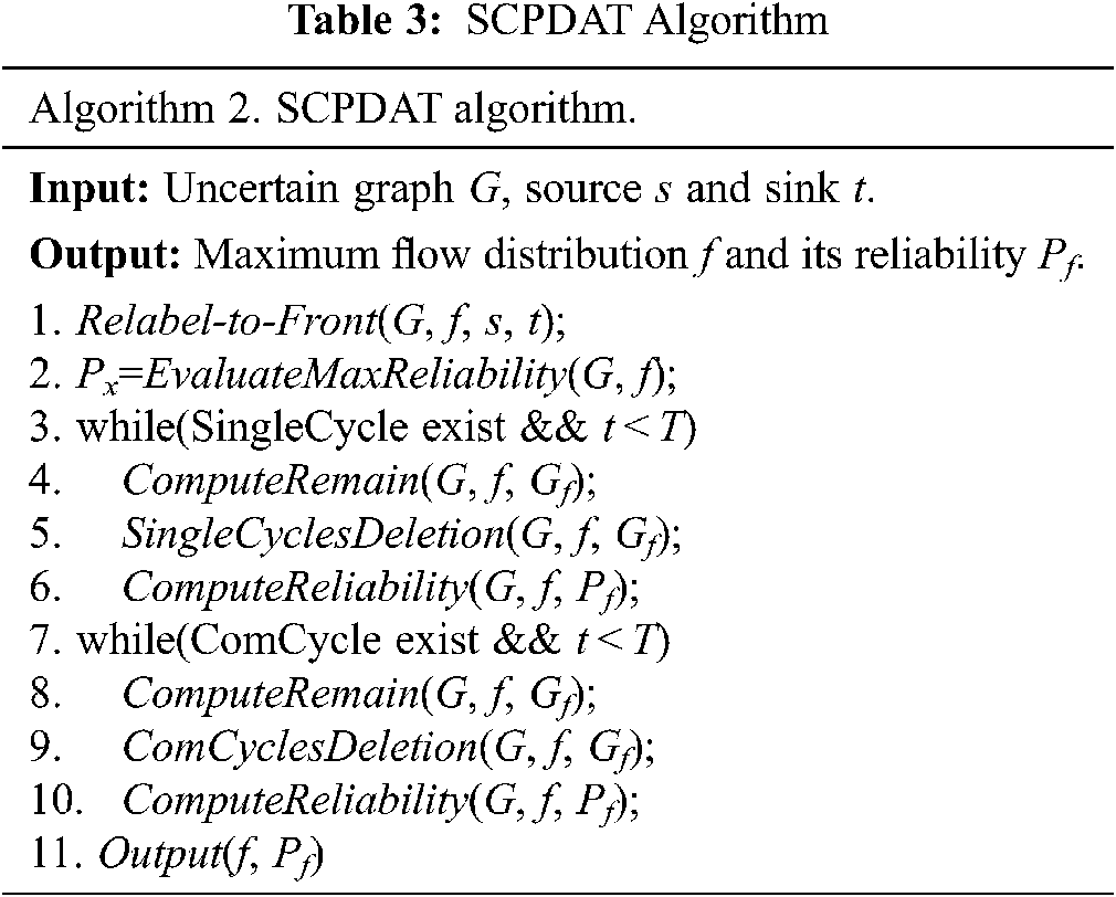
Similar to NWCD, SCPDAT first uses Relabel-to-Front to find a maximum flow distribution f and constructs the corresponding residual graph Gf. Subsequently, the function SingleCyclesDeletion is used to find and delete the negative weight communities composed of single cycles. When the single-cycle negative weight communities are all deleted, if there is still time remaining, the multi-cycle communities are deleted. Finally, the maximum flow distribution is obtained and the corresponding probability value is output.
According to the analysis in Section 2, the time complexity of the maximum flow algorithm in the first line is O(|V|3), while the time complexity of lines 3 to 6 (searching for and deleting the single-cycle negative weight communities) is O(|V|2|C|). Thus, the complexity of the first half of the algorithm is O(|V|3+ |V|2|C|). Lines 7 to 9 will be executed only if there is still time remaining, so the time complexity highly likely can be omitted.
5 The MRMF Approximation Algorithm Based on Single-Cycle Preference Deletion with a Probability Constraint
SCPDAP is also a type of single-cycle preference deletion algorithm. Unlike SCPDAT, SCPDAP uses the approximation degree of the optimal solution as a constraint. Searching for the remaining negative weight communities often takes a lot of time in the process of running NWCD, but the improvement in reliability is very limited. Thus, it is often not worth searching for and deleting the last few weight communities. In light of this, SCPDAP avoids spending a lot of time searching for and deleting negative weight communities owing to the limited improvement in reliability it provides.
5.1 Probability Threshold Setting
Similar to SCPDAT, the SCPDAP algorithm also deletes the single-cycle negative weight communities preferentially. Once all the single-cycle communities are deleted and the probability still has not reached the probability threshold, the multi-cycle negative weight communities will be found and deleted. The probability threshold is generally based on the specific requirements for reliability in practice; for example, it can be directly selected from the actual network that can provide the service well.
The algorithm implementation (pseudo-code) of SCPDAP is provided in Tab. 4.
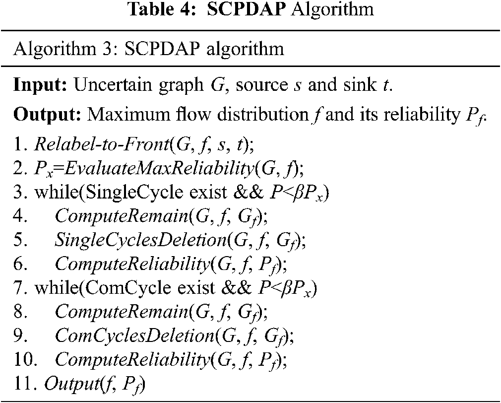
The algorithm also uses the Relabel-to-Front function to find a maximum flow distribution f and updates the corresponding residual graph Gf, after which the single-cycle communities are deleted. Only if the probability does not reach the threshold after all single-cycle communities have been deleted, multi-cycle communities will be deleted. The time complexity analysis is the same as for SCPDAT.
In order to verify the performance of the proposed algorithm, a series of experiments were carried out. These were divided into three main stages. In the first stage, performance comparisons of NWCD and SDBA were performed on synthetic datasets with different scales and densities. In the second stage, through grouped experiments, the approximation degree of the solution obtained by SCPDAT was recorded when it took 5%, 10%, 20%, and 40% of the NWCD’s time. This tested the effect of preferentially deleting a large proportion of single-cycle communities. In the third stage, when the probability threshold was set to 95%, 90%, and 85% of the probability of the optimal solution, the relationship between the accuracy loss and the time cost benefit in different datasets could be observed to test the effect of omitting part of the negative weighted communities.
6.1 Experimental Environment and Dataset
The experimental platform was an Intel Pentium (R) Dual PC (CPU E2180 2.00 GHz, 8GB memory, 32-bit Ubuntu12.04 operating system). The algorithm was written in C/C++ and the compiler environment was gcc4.6.3. To facilitate convenient comparison with SDBA (also transplanted to the Ubuntu version), the same dataset used in [17] was used in the present experiments. The dataset was divided into the following two groups:
(1) Generating V6A10, V8A14, V10A18, V12A22, and V14A26 (five group graphs) using the directed graph generator NETGEN [25], where VnAm denotes a graph set consisting of n vertices and m edges (in this experiment, the set size was between 5 and 20). Similar to [17], during the experiment, the points with the largest number of simple paths between any two points were selected as the endpoints; these were used as the source and sink points to ensure that there were as many paths as possible from s to t.
(2) The number of vertices in the graph was fixed (the number in the experiment was 14), and the number of edges was consistent with the graph density defined in [26]. The density t was equal to 2|A|/|V|×(|V|-1) (the density t was set to 0.25, 0.3, 0.35, 0.4, and 0.45 in the experiment). The graphs were generated by NETGEN. The capacity and the corresponding probability of the edges in the graph satisfied the random distribution, while the selection of the source and sink points was the same as in (1).
6.2 Algorithm Performance Comparison
The experiments compared the differences in the time performance, memory consumption and accuracy of various algorithms by using different datasets, different graph sizes, and different density conditions.
Experiment 1: A dataset of type (1) was selected. The capacity and corresponding probability in the graph were combined according to random, uniform and normal (σ = 0.2, 1.0, 1.8) distributions, and the performances of SDBA and NWCD were compared under different graph scales.
Fig. 5 presents a comparison between the capacity of the edge and the corresponding probability when the distribution was evenly distributed. The results showed that NWCD greatly improved in terms of time performance relative to SDBA. As the graph scale (edge number) increased, the time consumed by the two algorithms also increased. Moreover, as the number of edges increased, the state space of SDBA increased, meaning that the time consumed also increased quickly. The time consumed by NWCD also increased with an increasing number of edges. This was because the cycle structure in the uncertain graph would increase when the number of edges increased. However, NWCD still maintained a huge advantage over SDBA. Fig. 6 presents a comparison of the memory consumption of the two algorithms; both exhibited a small difference in space cost that increased with graph size.
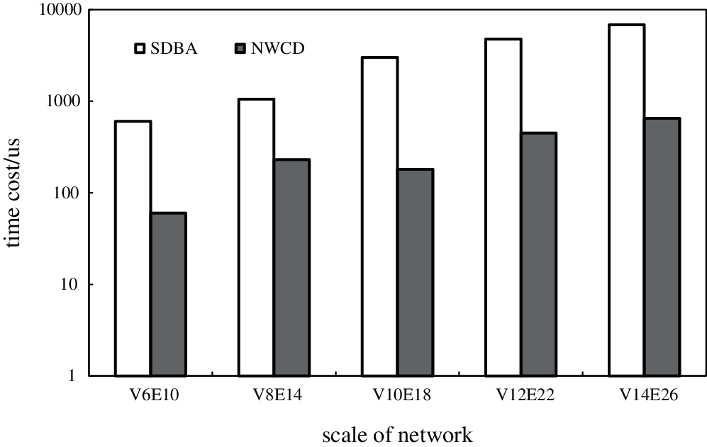
Figure 5: Relationship Between Time Cost and Network Scale
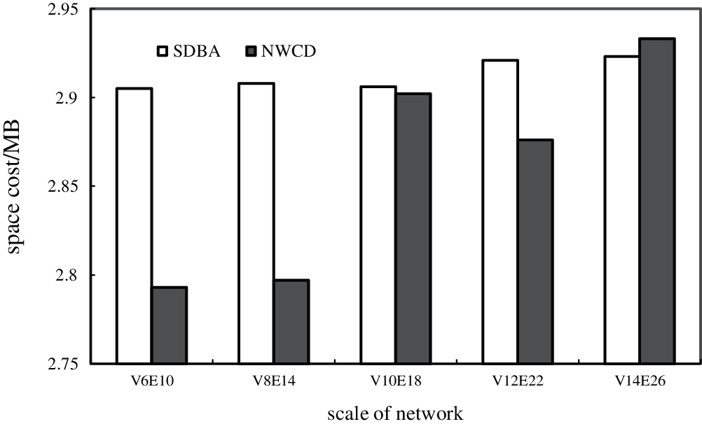
Figure 6: Relationship Between Memory Space Cost and Network Scale
Experiment 2: The dataset of type (2) was used to examine the effect of different densities on the performances of SDBA and NWCD.
Fig. 7 shows that when the number of vertices is the same (|A| = 14), the density of the edge increases from 0.3 to 0.5 with an increment of 0.05. As the density increases, the time performance of the two algorithms also generally increases. Compared with SDBA, the algorithm proposed in this paper exhibits a slower growth rate while maintaining a performance advantage.
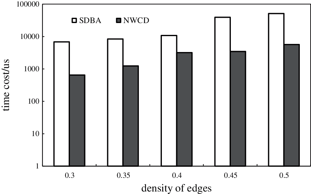
Figure 7: Relationship Between Time Cost and Edge Density
Experiment 3: Two datasets (V12A22 and V14A26) in the type (1) dataset (each set was expanded to 20; that is, each group contained 20 graphs with the same number of vertices and edges but different topologies) were selected to calculate the approximation degree of the solution obtained by SCPDAT separately, when it took 5%, 10%, 20%, 40% of the time of NWCD.
Fig. 8 shows that SCPDAT can spend less time in the initial stage finding and deleting large numbers of the single-cycle communities, and thus quickly obtains a better approximate distribution. In the latter stage, SCPDAT spends large amounts of time deleting the multi-cycle communities; however, the improvement in reliability is very limited. Therefore, if it is not necessary to find the optimal solution in a specific application, it is both meaningful and feasible to sacrifice some amount of accuracy to obtain a time cost saving. In addition, it was found that after spending 5%–20% of the time required to delete all single-cycle communities, a higher approximation degree of the solution (about 90%) could be obtained.
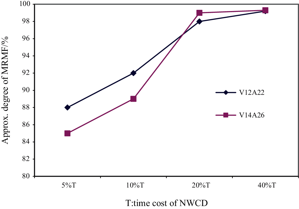
Figure 8: The Relationship Between Accuracy and Time Cost
Experiment 4: Two datasets (V12A22 and V14A26) of type (1) were selected to calculate the time taken by SCPDAP when the accuracy reached 95%, 90%, and 85% of the optimal solution.
Similar to the results of SCPDAT, Fig. 9 shows that if the accuracy of the algorithm is allowed to reduce appropriately, very substantial time cost savings can be made. This indicates the feasibility of omitting to delete some multi-cycle negative weight communities in order to obtain performance improvements for the algorithm.
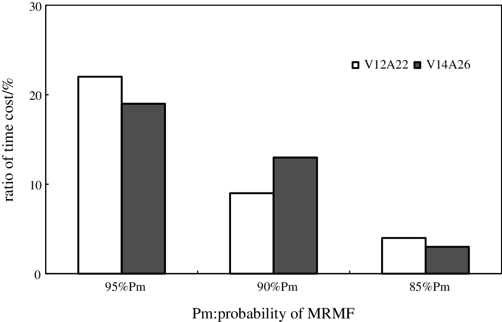
Figure 9: The Relationship Between Time Cost and Accuracy
In view of the relatively simple network structure of the edge nodes in the CDN, the “flow-shifting” algorithm of minimum cost and maximum flow is considered; thus, NWCD, SCPDAT and SCPDAP based on negative weight community deletion are proposed in this paper. NWCD continuously deletes the negative weight communities to increase the reliability until all negative weight communities are deleted, which results in the MRMF. Experiments show that, compared with SDBA, NWCD with probability pruning strategy achieves an order of magnitude increase in time performance. To further improve the performance of the algorithm, SCPDAT and SCPDAP are proposed on the basis of NWCD. Under specific constraints, these algorithms can obtain approximation solutions as quickly as possible by preferentially deleting single-cycle negative weight communities (which make up a large proportion of negative weight communities) and by avoiding searching for and deleting multi-cycle communities (which has a high time cost). Thus, it can meet the demands of some real-time applications.
Acknowledgement: The authors would like to thank the Editor and anonymous reviewers for their valuable comments that significantly improved the manuscript.
Funding Statement: This work was partly supported by Open Research Fund from State Key Laboratory of Smart Grid Protection and Control, China (Zhang B, https://www.byqsc.net/com/nrjt/), Rapid Support Project (61406190120, Zhang B), the Fundamental Research Funds for the Central Universities (2242021k10011, Zhang B, https://www.seu.edu.cn) and the National Key R&D Program of China (2018YFC0830200, Zhang B, https://www.most.gov.cn).
Conflicts of Interest: The authors declare that they have no conflicts of interest to report regarding the present study.
1. W. W. Zhu and Z. Wang, “Data-driven multimedia edge network and content delivery,” SCIENCE CHINA: Information Sciences, vol. 51, no. 3, pp. 468–504, 2021. [Google Scholar]
2. M. A. Salahuddin, J. Sahoo, R. Glitho, H. Elbiaze and W. Ajib, “A survey on content placement algorithms for cloud-based content delivery networks,” IEEE Access, vol. 6, no. 9, pp. 91–114, 2017. [Google Scholar]
3. H. B. Zhang, Y. Cheng, K. J. Liu and X. F. He, “The mobility management strategies by integrating mobile edge computing and CDN in vehicular networks,” Journal of Electronics and Information Technology, vol. 42, no. 6, pp. 1444–1451, 2020. [Google Scholar]
4. J. Sung, M. Kim, K. Lim and J. Rhee, “Efficient cache placement strategy in two-tier wireless content delivery network,” IEEE Transactions on Multimedia, vol. 18, no. 6, pp. 1163–1174, 2016. [Google Scholar]
5. M. Garmehi, M. Analoui, M. Pathan and R. Buyya, “An economic mechanism for request routing and resource allocation in hybrid CDN–P2P networks,” International Journal of Network Management, vol. 25, no. 6, pp. 375–393, 2015. [Google Scholar]
6. K. Xu, X. Li, S. K. Bose and G. X. Shen, “Joint replica server placement, content caching, and request load assignment in content delivery networks,” IEEE Access, vol. 6, no. 3, pp. 17968–17981, 2018. [Google Scholar]
7. J. Song and H. Sang, “The development and application of CDN technology,” Video Engineering, vol. 276, no. 6, pp. 75–77, 2005. [Google Scholar]
8. S. S. Sarma and S. K. Setua, “Uniform load sharing on a hierarchical content delivery network interconnection model,” Innovations in Systems & Software Engineering, vol. 12, no. 3, pp. 1–10, 2016. [Google Scholar]
9. P. Hintanen, H. Toivonen and P. Sevon, “Fast discovery of reliable subnetworks,” in Proc. the 11th Int. Conf. on Advances in Social Networks Analysis and Mining (ASONAMOdense, Denmark, pp. 104–111, 2010. [Google Scholar]
10. P. Hintsanen and H. Toivonen, “Finding reliable subgraphs from large probabilistic graphs,” Data Mining and Knowledge Discovery, vol. 17, no. 1, pp. 3–23, 2008. [Google Scholar]
11. Z. Zou, J. Li, H. Gao and S. Zhang, “Finding top-k maximal cliques in an uncertain graph,” in Proc. the IEEE 26th Int. Conf. on Date Engineering (ICDELong Beach, California, USA, pp. 649–652, 2010. [Google Scholar]
12. Z. Zou, J. Li, H. Gao and S. Zhang, “Mining frequent subgraph patterns from uncertain graph data,” IEEE Transactions on Knowledge and Data Engineering, vol. 22, no. 9, pp. 1203–1218, 2010. [Google Scholar]
13. C. Alexopoulos, “Note on state-space decomposition methods for analyzing stochastic flow network,” IEEE Transactions on Reliability, vol. 44, no. 2, pp. 354–357, 1995. [Google Scholar]
14. C. C. Jane and Y. W. Laih, “Computing multi-state two-terminal reliability through critical arc states that interrupt demand,” IEEE Transactions on Reliability, vol. 59, pp. 338–345, 2010. [Google Scholar]
15. J. E. Ramirez-Marquez and D. W. Coit, “A monte-carlo simulation approach for approximating multi-state two terminals reliability,” Reliability Engineering & System Safety, vol. 87, pp. 253–264, 2005. [Google Scholar]
16. Y. K. Lin, “System reliability evaluation for a multi-state supply chain network with failure nodes using minimal paths,” IEEE Transactions on Reliability, vol. 58, no. 1, pp. 34–40, 2009. [Google Scholar]
17. W. Cai, B. L. Zhang and J. H. Lv, “Algorithms of the most reliable maximum flow on uncertain graph,” Chinese Journal of Computers, vol. 35, no. 11, pp. 2371–2380, 2012 (in Chinese). [Google Scholar]
18. L. R. Ford and D. R. Fulkerson, “Flows in networks,” Physics Today, vol. 16, no. 7, pp. 54–56, 1962. [Google Scholar]
19. A. Y. Hamed, M. H. Alkinani and M. R. Hassan, “A genetic algorithm to solve capacity assignment problem in a flow network,” Computers, Materials & Continua, vol. 64, no. 3, pp. 1579–1586, 2020. [Google Scholar]
20. L. Yan, Y. H. Zheng and J. Cao, “Few-shot learning for short text classification, “ Multimedia Tools and Applications, vol vol. 77, pp. 29799–29810, 2018. [Google Scholar]
21. A. I. Al-Omari, I. M. Almanjahie and A. S. Hassan, “Estimation of the stress-strength reliability for exponentiated pareto distribution using median and ranked set sampling methods,” Computers, Materials & Continua, vol. 64, no. 2, pp. 835–857, 2020. [Google Scholar]
22. Y. Chen, Y. Tang, L. Zhou, Y. Zhou, J. Zhu et al., “Image denoising with adaptive weighted graph filtering,” computers,” Materials & Continua, vol. 64, no. 2, pp. 1219–1232, 2020. [Google Scholar]
23. Y. Yang, J. Wang, Z. Gao, Y. Huo and X. Qiu, “Sri-xdfm: A service reliability inference method based on deep neural network,” Intelligent Automation & Soft Computing, vol. 26, no.6, pp. 1459–1475, 2020. [Google Scholar]
24. A. V. Goldberg and R. E. Tarjan, “A new approach to the maximum flow problem,” Journal of the ACM, vol. 35, no. 4, pp. 921–940, 1988. [Google Scholar]
25. D. Klingman, A. Napier and J. Stutz, “NETGEN: A program for generating large scale capacitated assignment, transportation and minimal cost flow network problems,” Management Science, vol. 20, no. 5, pp. 814–821, 1974. [Google Scholar]
26. D. Johnson, “Finding all the elementary circuits of a directed graph,” SIAM Journal on Computing, vol. 4, no. 1, pp. 77–84, 1975. [Google Scholar]
 | This work is licensed under a Creative Commons Attribution 4.0 International License, which permits unrestricted use, distribution, and reproduction in any medium, provided the original work is properly cited. |