Computer Systems Science & Engineering DOI:10.32604/csse.2022.020685
Article

Parallel Cloth Simulation Using OpenGL Shading Language

Hongly Va1, Min-Hyung Choi2 and Min Hong3,*

1Department of Software Convergence, Soonchunhyang University, Asan, 31538, Korea
2Department of Computer Science and Engineering, University of Colorado Denver, Denver, CO 80217, USA
3Department of Computer Software Engineering, Soonchunhyang University, Asan, 31538, Korea
*Corresponding Author: Min Hong. Email: mhong@sch.ac.kr
Received: 03 June 2021; Accepted: 05 July 2021

Abstract: The primary goal of cloth simulation is to express object behavior in a realistic manner and achieve real-time performance by following the fundamental concept of physic. In general, the mass–spring system is applied to real-time cloth simulation with three types of springs. However, hard spring cloth simulation using the mass–spring system requires a small integration time-step in order to use a large stiffness coefficient. Furthermore, to obtain stable behavior, constraint enforcement is used instead of maintenance of the force of each spring. Constraint force computation involves a large sparse linear solving operation. Due to the large computation, we implement a cloth simulation using adaptive constraint activation and deactivation techniques that involve the mass–spring system and constraint enforcement method to prevent excessive elongation of cloth. At the same time, when the length of the spring is stretched or compressed over a defined threshold, adaptive constraint activation and deactivation method deactivates the spring and generate the implicit constraint. Traditional method that uses a serial process of the Central Processing Unit (CPU) to solve the system in every frame cannot handle the complex structure of clothmodel in real-time. Our simulation utilizes the Graphic Processing Unit (GPU) parallel processing with compute shader in OpenGL Shading Language (GLSL) to solve the system effectively. In this paper, we design and implement parallel method for cloth simulation, and experiment on the performance and behavior comparison of the mass–spring system, constraint enforcement, and adaptive constraint activation and deactivation techniques the using GPU-based parallel method.

Keywords: Adaptive constraint; cloth simulation; constraint enforcement; GLSL compute shader; mass–spring system; parallel GPU

1  Introduction

The applications of physically based simulation have been widely applied in many industries, including film or animation, education, games, health care, and AR application. The main goal of physically-based simulation is to simulate rigid and non-rigid objects that interact and behave like their real-world counterparts [1]. When modeling and simulating 3D objects, the fundamental concepts of physical behavior, such as Newton’s law of motion and universal gravitational law, should be respected. In contrast, in order to construct realistic real-time models, interactive simulation of cloth has been studied for decades. The main purpose of cloth simulation is efficient, unconditionally stable, and real-time performance (higher than 30 frames per second). In some situations, cloth simulation turns to a stiff system that is strongly resistant to stretching motions. Alternatively, the mass–spring system (MSS) which is applied in interactive game application, is fast and simple to implement. However, it is difficult for the MSS to find the proper spring coefficients and a suitable integration time-step is required. The core idea behind the mass–spring system of cloth simulation is that it is based on particle simulation with the cloth object, treating the cloth as a grid of nodes. The grid is the connection between node or particle and its neighbor, and is known as a spring to resist forces from pulling apart when internal and external force are applied. The mass–spring damper model uses three types of springs (structural, shear, and bending) to preserve the cloth behavior [2]. However, when large time-step and stiffness coefficient are used, the spring force exhibits numerical instability, which results in the elasticity effect or blow-up situation, and in order to maintain the restriction of node-to-node distance, constraint force is used instead.

Since the computing and rendering a deformable cloth object is remarkably challenging and time-consuming, the level of detail in the cloth object has been optimized to achieve the real-time performance and realistic visual appearance [3]. The naïve algorithm of cloth simulation that use a serial process of a CPU to compute force and find a new position in every frame cannot handle the complex structure of cloth simulation in real-time. Parallel processing using the graphic processing unit (GPU) has been considered for the cloth simulation since it operates on multi-cores and thousands of threads in massive parallelism [4]. The single instruction multiple data (SIMD) architecture is a well-known model, due to its effective results in terms of latency, bandwidth, and memory accessing. Nonetheless, additional general purpose of computing on graphic processing unit (GPGPU) programs or libraries such as CUDA or OpenCL is required to utilize parallel GPU [5]. Therefore, OpenGL is used for rendering, so the additional GPGPU program or library can be excluded, since GLSL can be utilized to perform parallel processing of the cloth simulation by using OpenGL compute shader as a GPU kernel program.

In this paper, we present the implementation of cloth simulation using OpenGL shading language as a GPU-based parallel program. The specific contributions of our paper are:

•   Cloth simulation is implemented based on the mass–spring system, implicit constraint enforcement, and adaptive constraint activation and deactivation, using the compute shader.

•   The parallel method of sparse linear solving algorithm is utilized to accelerate cloth simulation using implicit constraint enforcement.

The performance comparison result of the cloth simulation using the mass–spring system, constraint enforcement and adaptive constraint activation and deactivation method that are implemented on GLSL compute shader are provided as well. In order to compare and contrast each method understandably, we conduct an experiment on the scenario that the cloth receives a strong force pushing the cloth object.

2  Related Work

Previous approaches related to the method of cloth simulation have been researched to represent the deformable cloth object in real-time. Finite element method (FEM) is a time-consuming method, due to the method obtaining an accurate result. Therefore, to accelerate the performance, Rodriguez-Navarro et al. [6] implemented a cloth simulation system based on FEM in the GPU. However, FEM required heavy computation to return an accurate result. Müller et al. [7] applied a position-based dynamic method to simulate the cloth object. The position-based method ignores the velocity and force properties, which directly displace the position of each node. Alternatively, the force-based method accumulates internal and external forces, and computes the acceleration based on Newton’s second law of motion. The time integration method is then used to update the velocities and the positions of the object, respectively. Generally, the force-based method of the mass–spring system was introduced and was further developed to achieve realistic and real-time modelling [8–10]. Parallel cloth simulation was implemented using OpenGL GLSL 4.3 [11]. However, additional operation is required to sum the forces of all springs that are connected to the mass node. Therefore, in order to compute the spring force using parallel GPU, the node-centric algorithm was proposed [12]. In order to displace each node in the spring to become the rest length of the spring at each given time-step, a dynamic inverse constraint on springs that were over-elongated was applied [8]. The distance reduction was applied on springs that could stretch more or compress less than a threshold of ± 10% of the spring rest length. However, the displacement of each node directly ignores the physical consequence of the dynamic behavior of motion. In order to prevent the excessive elongation of springs, implicit constraints are put to constrain the length of elongated springs beyond 10% [13].

3  Preliminaries

3.1 Mass–Spring System

Fig. 1 shows the three types of spring structure the mass–spring model uses, in order to maintain the overall cloth shape:

Figure 1: Three types of springs structure of the mass–spring model

Each spring is created by two nodes, where the positions of those two nodes are denoted by p1& p2, and v1& v2 are the velocities. f1& f2 are the forces acting on both nodes to keep the original shape of the spring. In contrast, spring force is added to adjust the stretching or compressing spring to the initial spring with initial distance or rest length L0, as illustrated in Fig. 2:

Figure 2: Stretching behavior of a single spring

Force acting on both nodes is known as spring force, which can be computed using Hooke’s law, as shows in Eq. (1) and Eq. (2). Parameter ks is the spring stiffness coefficient, and together with the damping coefficient kd is used to compute the spring force [12]:

f1=−[ks(|p1−p2|−L0)+kd((v1−v2)⋅(p1−p2)|p1−p2|)]p1−p2|p1−p2| (1)

f2=−f1 (2)

The motion of equations using the explicit Euler integration method is applied to update the node’s position p and velocity v at time t + Δt, where Δt is an integration time-step.

p(t+Δt)=p(t)+v(t+Δt)×Δt (3)

v(t+Δt)=v(t)+(gravity+FM)×Δt (4)

3.2 Implicit Constraint Enforcement

Hong et al. [13] use the future time-step in the implicit constraint enforcement method to estimate the correct magnitude of the constraint forces. q represents a list of position with size of 3n, and n is the total number of nodes within the cloth model q = [x1, y1, z1, x2, y2, z2… xn, yn, zn]T. Then Φ(q(t),t) is a constraint vector of m Algebraic constraint, while Φi is a scalar algebraic constraint equation. This distance constraint can be defined by the following equation:

Φ=(x1−x2)2+(y1−y2)2+(z1−z2)2−r2 (5)

Φ(q,t)= [Φ1(q,t),Φ2(q,t)…Φm(q,t)]T (6)

The system of equation can be written as follows in Eq. (7):

Mq¨+ΦqTλ=FA (7)

In the constraint optimization problem, the implicit constraint has to solve the problem Φ(q,t)= 0 . M is the mass matrix which is the diagonal element that stores the node’s mass, FA is the accumulation of gravity force and constraint forces interacting with the node, λ is the Lagrange multiplier vector with m size, and Φq is the Jacobian matrix size of m×3n, which is made by partial differentiation with respect to q [14]. The kinematic relationship between q and q˙ , as well as the equation of motion can be defined as follows equation:

q(t+Δt)=q(t)+ΔtM−1ΦqTλ+ΔtM−1FA(q, t) (8)

q(t+Δt)=q(t)+Δtq˙(t+Δt) (9)

The constraint function of next time is treated implicitly, and defined by Eq. (10) as follows:

Φ(q(t+Δt),t+Δt)=0 (10)

By using a truncated first order Taylor series to approximate Eqs. (10), (11) is obtained:

Φ(q(t),t)+Φq(q(t),t)(q(t+Δt)−q(t))+Φt(q(t),t)Δt=0 (11)

Substituting of Eqs. (8) & (9) into Eq. (11) can eliminate q(t + Δt):

Φq(q,t)M−1ΦqTλ=1Δt2Φ(q,t)+1ΔtΦt(q,t)+Φq(q,t)(1Δtq˙(t)+M−1FA(q,t)) (12)

Eq. (12) can be expressed by Ax = B, a sparse linear system, where A is the coefficient sparse matrix, B the right-hand side vector, and x is a Lagrange multiplier solved by the direct or iterative method. In contrast, a precise and effective algorithm is required in order to solve the system.

3.3 Compute Shader

In OpenGL 4.3 core, GLSL provides the possibility for parallel computing advantage by using the graphic processing unit (GPU) without an additional environment configuration, and executes in different pipeline with the rendering pipeline [15]. ACompute shader is a shader that uses GLSL based on the syntax of C programming language similar to vertex or fragment shader, Compute shader can be executed using the glDispatchCompute() command with a given workgroup dimension block in three dimensions. Since compute shader is executed on the GPU with massive parallelism, compute space is required to accelerate the computation performance. Designing and implementing the compute space of compute shader is dependent on the problem and type of data. Fig. 3 shows the scheme of compute space dimension.

Figure 3: The compute space of compute shader

Compute space consists of three-dimensions of the workgroup, with each element of the workgroup consisting of a local workgroup. A single local workgroup is a group of invocations or threads that is defined as 1D, 2D, and 3D in compute shader. Furthermore, compute shader program executes for all invocations in non-sequential order in parallel GPU. Correspondingly, shared memory can be accessed for any invocation within the same local workgroup as well. Compute shader can use the uniform variables that are declared in OpenGL’s function. There are limitations on the local workgroup size due to the specification of hardware.

Shader Storage Buffer Object (SSBO) is OpenGL’s buffer object for incoherent memory access. SSBO is used to store extremely large arrays of structured data. It can share data between different program (compute shader). There are two standard layout qualifiers of buffer in compute shader to be concerned with, due to the rule of memory offset per data block [16]. Fig. 4 illustrates the rules of the standard layout qualifier of buffer. The first standard layout qualifier is std 140, which is required padding data in order to pack elements into one block of the buffer, so an array of type has to be mapped before initializing the SSBO. Differently, the other one of the standard layout qualifiers, std 430 does not require offset data for packing element to buffer. This also means, an array of float in C/C++ is tightly packed directly into a buffer.

Figure 4: SSBO memory layout qualifiers’ rule

4  Implementation of Cloth Simulation

In this paper, parallel cloth simulation is implemented using the mass–spring method, constraint enforcement method, and adaptive constraint activation/deactivation method for performance and behavior comparison. Information related to simulation such as the node’s position, velocity, and force, are stored in SSBO, due to task distribution of compute shader and the Single Instruction Multiple Data (SIMD) architecture of the GPU. Initial data of SSBO are required in order to start the simulation as well.

4.1 Mass–Spring System on the GPU

A single node or particle possibility has 6 spring connections (2 structure, 2 shear and 2 bend springs) or 12 directions of force in total where 6 directions of force act on another node, and 6 directions of force are received from another node. Fig. 5 demonstrates the direction of spring in the mass–spring structure.

Figure 5: Structure of spring direction

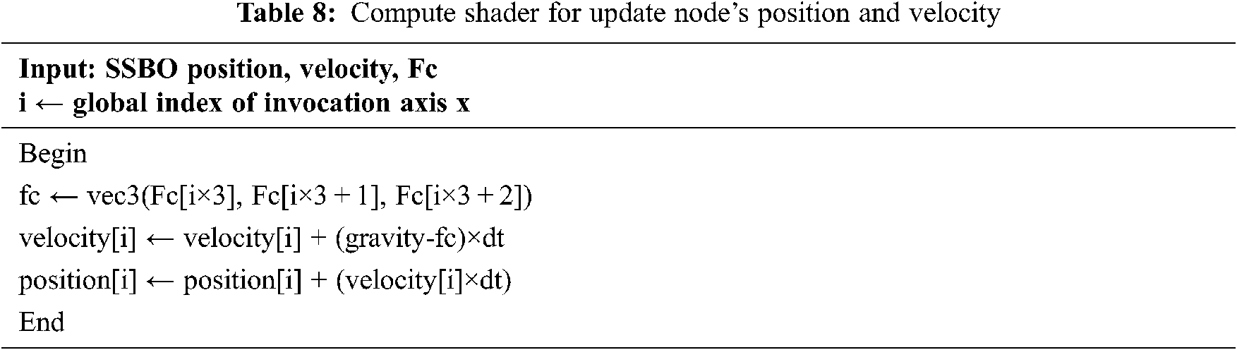
The nodes in a cloth model located as 2D structure, 2D workgroup are used to access the node information storing in SSBO through the index of invocation. We define the size of the local workgroup as (x = 16, y = 16, z = 1), to accumulate spring force in compute shader. Two nodes are required to compute the spring force by Eq. (1). Since SSBO is stored in the 1D array of data, global index is computed to invoke data in SSBO. Tab. 1 shows how compute shader computes the spring force on the particle or node. After particle force computation, the new node’s position can be computed as well. We use only 1D workgroup to update nodes with local workgroup dimension determined as (x = 1,024, y = 1, z = 1). The global workgroup dimension is used to dispatch compute shader program. Tab. 2 shows the compute shader pseudo code to update each node’s position and velocity.

4.2 Constraint Enforcement on the GPU

The Constraint force computation requires complex and large data storage. So, we use SSBO to contain data of the constraint enforcement simulation, as shown in Tab. 3. In regard to the initializing stage, the SSBO requires the size of the buffer to be pre-defined before the simulation starts as well. The partial differentiation of distance constraint function yields a Jacobian matrix (J), which is a structured sparse matrix. Generally, dense matrix is used for storing the matrix element that contains all zeros and non-zero elements in a 2D array structure. The general operation of dense matrix is a time-consuming operation, so sparse matrix is used instead to optimize memory allocation and general operation. Under these circumstances, we applied Compressed Sparse Row (CSR) format to store the Jacobian matrix and Compressed Sparse Column (CSC) to store its transpose (JT) without additional transposing operation on sparse matrix. While the row number of the Jacobian matrix is equal to the number of constraints and each row of the Jacobian matrix possibility consists of six non-zero values, the SSBO size to store sparse matrix is 6-by-constraints and the compressed row or column index is equal to constraints plus 1.

Coordinate (COO) format is used for the system matrix, since it is commonly used for storing unstructured sparse matrix and using a simple structure of triplet (row, column, non-zero value) as storage. The size of the system matrix is implicit, which requires pre-computing of the size to initialize the SSBO of the COO matrix.

Multiple processes of constraint force computation are distributed into sub-process by using multiple compute shaders. Tab. 4 shows the list of compute shader for cloth simulation using constraint enforcement. Each compute shader uses a different number of workgroups, due to the size of data.

disConstraint() compute shader is used to compute Φt(q, t) and construct SSBO Phi as well. At the same time, a row of the Jacobian matrix is formulated and stored in CSR SSBO (A, IA, and JA), and the transpose of the Jacobian matrix CSC SSBO (B, IB, and JB) by using one innovation in the compute space of compute shader. Vect() compute shader is used to compute vector (1Δtq˙(t)+M−1FA(q,t)) . Hence, Rhs() compute shader is used to compute right-hand side of the system ( 1Δt2Φ(q,t)+1ΔtΦt(q,t)+Φq(q,t)(1Δtq˙(t)+M−1FA(q,t))) . Consequently Rhs() compute shader computes the result using sparse matrix–vector multiplication (SpMV) of CSR sparse matrix as shown in Tab. 5.

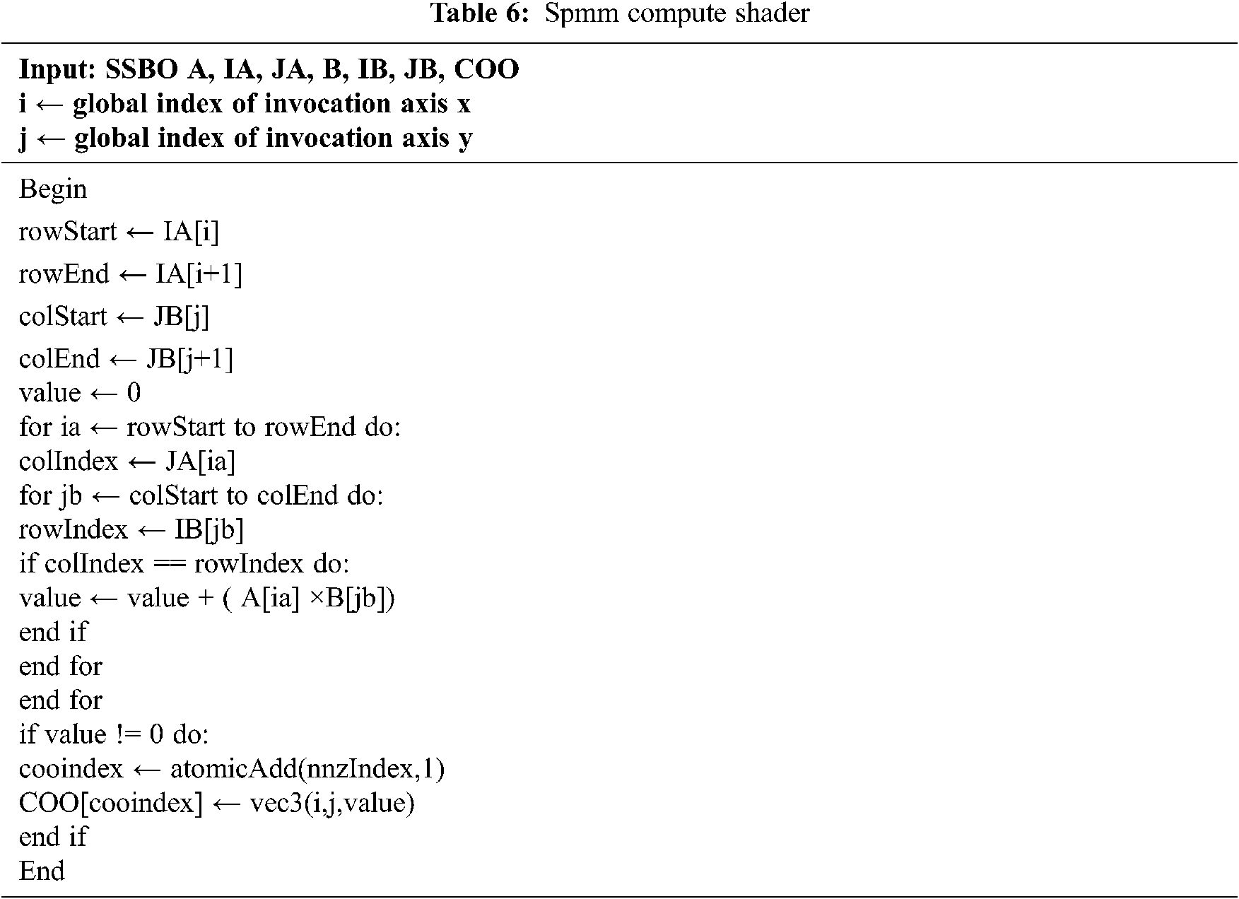
System matrix computation is the most critical operation in the simulation that requires an efficient and precise algorithm. We proposed the parallel algorithm for sparse matrix–matrix multiplication (SpMM) of CSR format and CSC format by utilizing GPU library, such as atomic operations. Since, compute shader processes data in parallel, an index of the new matrix element is increased by using atomic counter as well. Each non-zero element result stores a triplet data (row, column, and non-zero value) in vector of 3 or vec3 in GLSL at the index from the atomic counter result respectively. Spmm() compute shader is called to obtain the system matrix result. Tab. 6 shows SpMM algorithm.

In previous study, we implemented the Conjugate Gradient (CG) algorithm on GPU by using compute shader, given sparse matrix and right-hand side vector SSBO as input in order to find the λ vector with user defined iteration number [17]. The usage of a sparse matrix is extremely fast operating and saves much memory compared to dense matrix. In contrast, the number of iterations used for handling the tolerance factor of the system and the system can be converged in case the residual error is tiny enough. The convergence of the system produces a behavior of cloth that is strongly resistant and hard to stretch. There are three main operations of the CG algorithm, which consist of SpMV using COO sparse matrix, AxPY vectorization operation, and vector dot product. Generally, we can use atomic operation such as atomicAdd(), to concurrently sum SSBO data to perform parallel vector dot product. However, using an atomic operation requires locking step of the process in GPU, which can slow down the entire algorithm, so we consider using parallel sum reduction in shared memory using compute shader to accelerate the algorithm.

The vector dot product algorithm legitimately uses parallel sum reduction per workgroup with shared memory to accelerate the computation. The parallel dot product of the vector can be done by passing data of SSBO as global memory to shared memory and sum data using a stride index in the inner loop to obtain the final result. Additional global memory has to be reserved as well, in case SSBO is larger than the bounding size of shared memory or the maximum size of the local workgroup, since a local workgroup can obtain only a single element result. Fig. 6 illustrates the algorithm of parallel sum reduction on shared memory using compute shader.

Figure 6: Parallel sum reduction in shared memory

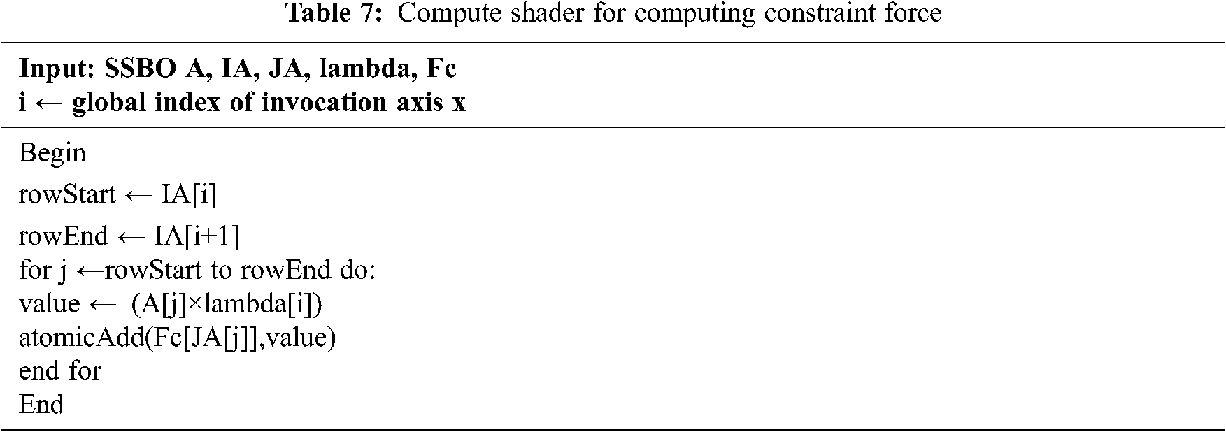
Consequently, ConstraintForce() compute shader is executed to compute the force based on Eq. (7). Steinberger [18] applied the SpMVT algorithm to multiply the transpose of matrix with vector. The operation involved SpMV of transpose matrix using a CSR format, as shown in Tab. 7. New velocity and position in the next frame are computed by Eqs. (8) & (9) in UpdateNodes() compute shader, as shown in Tab. 8.

4.3 Adaptive Constraint Activation and Deactivation Method on the GPU

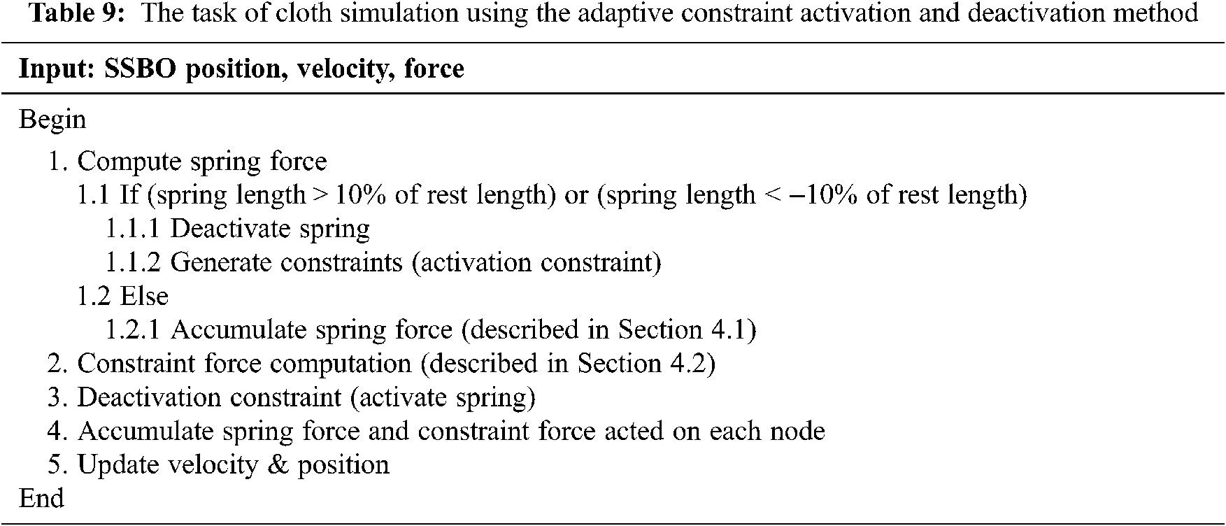
The adaptive constraint activation and deactivation method involves both mass–spring system and constraint enforcement, since a spring can be compressed or stretched in each frame of the simulation, which requires the desired force to prevent the elongation of spring. Our system initializes with the mass–spring system, which computes the force acting on node or particle; at the same time, we compute the length of that spring stretching or compressing. If the length reaches a threshold value (±10%), the spring is deactivated and that spring change to an implicit constraint. Consequently, constraint force computation is done corresponding to implicit constraint as well. Constraint force and spring force acting on the particle are accumulated and applied, in order to update the position and velocity. Tab. 9 demonstrates the task of cloth simulation using the adaptive constraint activation and deactivation method on the GPU.

5  Experimental Result

In this paper, the experiments were conducted on Windows platform with the following specification: CPU i7–7700 3.60 GHz, 16 GB RAM, NVIDIA GeForce GTX 1070 8GB V-RAM and Microsoft Visual Studio 2013 OpenGL 4.3. In order to get a fair comparison, the vertical synchronization is deactivated.

Tab. 10 compares the performance result between CPU-based and GPU-based algorithm with different resolution of cloth object wheren is the number of nodes and s is the number of springs, respectively. The result show that the GPU-based parallel mass–spring system is onaverage 61 times faster than CPU-based mass–spring system single core. Another comparison shows that the GPU-based constraint enforcementis on average 124 times faster, which is faster than the naïve approach that is implemented on the CPU single core. This comparison deliverssignificantly better results due to the GPU-based algorithm using compute shader, which is extremely fast, and runs on thousands of threads inparallel. The algorithm implemented on CPU consists of many loop operations in each frame of the simulation, and uses the serial process, so it causes slower performance result, compared to the parallel processing of the GPU-based algorithm

We also provide the peak performance result of cloth simulation using the mass–spring method, constraint enforcement, and adaptive constraint activation and deactivation method. Fig. 7 shows the cloth simulation performance using mass–spring. Since constraint enforcement is stable and accurate, we ignore the bending spring type to perform cloth simulation. However, without using bending spring type, the linear solving part of constraint force computation requires more iterations, compared to using all types of spring. Fig. 8 demonstrates the performance results of cloth simulation using the constraint enforcement method with different resolution of cloth model. The number of constraints in the cloth model that use all types of spring and only 2 types of spring are defined by s1 & s2, respectively.

Figure 7: Performance results of the mass–spring system measured in Frames Per Second (FPS)

Figure 8: Performance results of the constraint enforcement method measured in Frames Per Second (FPS)

In terms of performance, the mass–spring system is extremely faster than the other two methods, since it provided real-time performance for the cloth model that has a resolution of 5,242,880 nodes and 31,434,242 springs. On the other hand, the constraint enforcement method attempts to solve complex and large system in real-time, which requires a parallel algorithm to perform the simulation. The performance of cloth simulation using the constraint enforcement method can handle the resolution of 2,704 nodes and 10,506 springs in real-time. Applying the adaptive constraint activation and deactivation method to the simulation delivers significantly better results, compared to the constraint enforcement method. In Fig. 9, the peak performance of cloth simulation in real-time can handle about 16,384 nodes and 97,026 springs.

Figure 9: Performance results of the adaptive constraint method measured in Frames Per Second (FPS)

In order to contrast the efficiency of each method, Fig. 10 compare behavior of the cloth model when strong force is applied to a cloth object. The first row shows snapshots of cloth simulation using the mass–spring system method. The second row shows snapshots of cloth simulations using the constraint enforcement method. The third row shows snapshots of cloth simulations using our proposed method, which applied the adaptive constraint activation and deactivation techniques.

Figure 10: Cloth simulation behavior result when the cloth receives strong force pushing from the bottom of the cloth (time-step = 0.005)

A blow-up situation happened in cloth simulation using the mass–spring system with large time-step and stiffness coefficient. Conversely, constraint enforcement is stable, and represents the behavior of cloth that is hard to stretch and strongly resisted even strong force applied to the cloth model. Likewise, the adaptive constraint activation and deactivation method also produced excellent behavior of the cloth model when it receives strong force.

Fig. 11 demonstrates the different behavior of the cloth model using constraint enforcement and our proposed approach with various time-step. The simulation results demonstrate two points. First, cloth simulation using constraint enforcement is stable while using time-step = 0.02. So, an apparent limitation of the method is using time-step smaller than 0.02. Second, the adaptive constraint activation and deactivation technique consist of numerical error that cause weird behavior during simulation when using time-step = 0.02. However, when using time-step = 0.01, the adaptive constraint method of the simulation obtains a good result. Regarding this limitation, the cloth simulation using adaptive constraint activation and deactivation should be applied at most time-step dt = 0.01 for better result.

Figure 11: Cloth simulation behavior result using the large timestep

6  Conclusion

In this paper, we designed and implemented cloth simulation based on the mass–spring system, constraint enforcement method, and adaptive constraint activation and deactivation using the parallel structure of OpenGL GLSL 4.3 compute shader as a GPU kernel program. The method of the mass–spring system required a small integration time-step in order to achieve stable and effective behavior. Therefore, the constraint-based method provides stable and effective control of cloth behavior, which can be used with large integration time-step. We proposed the adaptive constraint activation and deactivation technique to reduce the computational burden, and using GPU-based parallel processing to accelerate the performance in real-time. Due to the usage of the parallel method of sparse linear solving (CG method), the performance of cloth simulation using implicit constraint enforcement implemented on the GPU is faster than CPU-based implementation by about 124 times.

There are several limitations to the proposed approach. In the constraint enforcement scheme, the number of buffer size is pre-computed to optimize the compute space in the GPU. Since our purposed approach utilized floating point atomic operation, which is provided by the NVIDIA GPU, different GPUs may not run our simulation well. Similarly, the maximum size of compute space and size of shared memory can differ, depending on the specification of the GPU.

In future work, we will optimize the performance result of constraint enforcement by using a variety of sparse matrix–matrix multiplication algorithms, since that is the time-consuming operation in the simulation. In addition, we will look into different options to avoid the use of atomic operation in the simulation. Regardless, future research could continue to explore the numbers of workgroup to increase simulation performance as well. Furthermore, the simulation system using parallel GPU on AR/VR device can achieve better performance without reducing levels of detail of object comparability to the method using serial process.

Funding Statement: This work was supported by the Basic Science Research Program through the National Research Foundation of Korea (NRF-2019R1F1A1062752), funded by the Ministry of Education; was funded by BK21 FOUR (Fostering Outstanding Universities for Research) (No.: 5199990914048); and was also supported by the Soonchunhyang University Research Fund.

Conflicts of Interest: The authors declare that they have no conflicts of interest to report regarding the present study.

This work is licensed under a Creative Commons Attribution 4.0 International License, which permits unrestricted use, distribution, and reproduction in any medium, provided the original work is properly cited.