Computer Systems Science & Engineering DOI:10.32604/csse.2022.020810
Article

Brain Image Classification Using Time Frequency Extraction with Histogram Intensity Similarity

Thangavel Renukadevi1,*, Kuppusamy Saraswathi1, P. Prabu2 and K. Venkatachalam3

1Department of Computer Technology-UG, Kongu Engineering College, Erode, India
2Department of Computer Science, CHRIST (Deemed to be University), Bengaluru, India
3Department of Computer Science and Engineering, CHRIST (Deemed to be University), Bengaluru, India
*Corresponding Author: Thangavel Renukadevi. Email: renuka.ctug@kongu.edu
Received: 09 June 2021; Accepted: 22 July 2021

Abstract: Brain medical image classification is an essential procedure in Computer-Aided Diagnosis (CAD) systems. Conventional methods depend specifically on the local or global features. Several fusion methods have also been developed, most of which are problem-distinct and have shown to be highly favorable in medical images. However, intensity-specific images are not extracted. The recent deep learning methods ensure an efficient means to design an end-to-end model that produces final classification accuracy with brain medical images, compromising normalization. To solve these classification problems, in this paper, Histogram and Time-frequency Differential Deep (HTF-DD) method for medical image classification using Brain Magnetic Resonance Image (MRI) is presented. The construction of the proposed method involves the following steps. First, a deep Convolutional Neural Network (CNN) is trained as a pooled feature mapping in a supervised manner and the result that it obtains are standardized intensified pre-processed features for extraction. Second, a set of time-frequency features are extracted based on time signal and frequency signal of medical images to obtain time-frequency maps. Finally, an efficient model that is based on Differential Deep Learning is designed for obtaining different classes. The proposed model is evaluated using National Biomedical Imaging Archive (NBIA) images and validation of computational time, computational overhead and classification accuracy for varied Brain MRI has been done.

Keywords: Histogram; differential deep learning; convolutional neural network

1  Introduction

Machine learning algorithms have the prospective to be reviewed enormously in all areas of medicine, from medication finding to clinical decision making, extensively changing the way the medicine is consumed. The progress of machine learning materials and methods at computer vision chores in the current era has favorable time when medical records are progressively digitalized. Therefore medical images are found to be an essential part of patient’s Electronic Health Records (EHRs) and examined by human radiologists, who are found to be constrained specifically by momentum, tiredness and experience. Hence a delayed or incorrect diagnosis causes harm to the patient. In a novel CNN based approach with the objective of classifying the sub-cortical brain structured in an accurate manner integrating both the convolution and prior spatial features is presented and classification accuracy is also said to be improved. With the objective of improving and enhancing the accuracy rate of the automated classification, the network is trained by means of a restricted sample selection. With this, the most significant and inherent structure parts are also learnt. Despite the improvement found in the accuracy, the computational complexity involved in measuring intensity and therefore the error rate are not detailed in [1]. To address this issue, in the present study, Histogram Intensity-oriented Pre-processing model that obtains standardized pre-processed features, thereby reducing the error rate by mapping the image scale and standard scale by means of normalization function is presented. Further, with the standardized pre-processed features, the error rate is said to be also reduced with the reduction in the complexity by transforming pre-processed brain MRI to time-frequency features.

Several medical image segmentation models are designed on the basis of the voxel classification in a supervised manner. Such methods usually execute well when given with a training set that is characteristic of the test images to segment. However, with different distributions being followed for training and test data, the problem is said to arise.

A kernel learning method was investigated in [2] to minimize the discrepancy between training data and test data and to measure the added value of kernel learning for weighting the corresponding images. A new image weighting method is also presented to reduce the Maximum Mean Discrepancy (MMD) between training and test data. In this way, an integrated optimization of image weights and kernel is said to be achieved. Despite the error arising due to MMD is found to be reduced, with the variance normalization constraint, many number of classifiers are not said to be formed and therefore compromising the accuracy. To address this issue, in the present study, a Softmax medical image classification is applied to the time-frequency features extracted, therefore minimizing the variance and hence improving the medical image classification accuracy rate.

The main importance of this research work is time frequency feature extraction from brain MRI images by reducing the variance of normalization and improving classification accuracy. The organization of the paper is as follows. Discussion of prior research work on brain MR image classification and the contribution of the present study are summarized in Section 2. In Section 3, the proposed methodology for brain MR image classification is presented. In Section 4, the effectiveness of the method is experimentally analyzed using the Brain MR images from NBIA. In Section 5, the concluding remarks are provided.

2  Related Works

Segmentation and the successive evaluation of lesions in medical images give an insight into information for analyzing neuropathology’s and are significant for designing strategies for treatment, disease monitoring and patient prediction results. For a thorough comprehension of pathophysiology, quantitative imaging provides the physicians with several most relevant indications pertaining to the disease characteristics and the pros and cons on specific anatomical structures.

And, the recent research related to the brain image classification includes the implementation of 3D CNN techniques. The three dimensional values include length, depth and height to generate activation maps, which merges inert medical image intensities with spatial framework. And, 3D CNN techniques have wide variety of applications in lung nodule detection, Alzheimer disease identification, brain disorder in infants, etc., The usage of CNN in methodologies such as segmentation, classification, retrieval using brain, chest, lung, colon and liver images are analyzed. The challenges involved in implementation of CNN in various modalities and idea for future research has been discussed in [3].

Also, Hierarchical Medical Image Classification (HMIC) approach has been used for multi-class classification of biopsy images. Hierarchical structures of CNN architecture are generated to improve the performance of multi-class classifier is presented in [4].

Deep learning is applied in CT images for classifying pulmonary artery vein [5] by means of 3D CNNs. With this, the classification accuracy is found to be better and achieved 94% accuracy. However, CNNs possess attributes and insufficient training samples which results in over-fitting and poor generalization. To address this issue, a novel dual loss function [6] is designed ensuring both cardiac segmentation and disease diagnosis. A novel variant of Bag of Words for medical image classification using chest images is presented in [7].

Segmenting medical images, pixel identification from background medical images involving CT or MRI images, is considered to be one of the most significant tasks in medical image processing for delivering most vital information pertaining to organ shapes and volumes. In [8], deep learning techniques are applied and the challenges involved are also addressed. However, the computational complexity involved in classification is found to be high. To address this issue, in [9], connected random field is introduced to remove the false positive and it is proved to be computationally efficient. Yet another work based on CNN is presented in [10] from cardiac images, therefore improving accuracy.

The differentiation between images acquired via different scanners or different imaging techniques provides a protocol that presents a paramount threat in automatic biomedical image classification. Transfer learning is designed in [11], which can train a classification scheme by means of multi-site data, consequently minimizing the classification error. However, the intra class and inter class variations are not said to be addressed. To address this issue, a Large Margin Local Estimate (LBLE) classification model is presented in [12]. Despite improving the accuracy and minimizing the error, automated detection is not possible. Further, a two stage method using Deep CNN is proposed in [13].

Fusion of preceding awareness pertaining to organ shape and location is paramount to enhance the performance of image analysis. However, in most current and favorable methods like CNN-based segmentation, it is not crystal clear how to integrate such prior knowledge. A novel method incorporating prior knowledge in CNN by means of regularization model is presented in [14] and obtained 83.3% accuracy. An ensemble of classification models maximizing the likelihood function also is proposed in [15].

Strong and swift solutions for detecting anatomical object and object segmentation contribute to the overall configuration starting from disease diagnosis, patient satisfaction and planning therapy to the feedback process. Marginal Space Deep Learning that combines both the advantages of object parameterization and automated feature design, therefore improving classification accuracy, is introduced in [16]. Classification of retinal imaging data is done in [17]. In this, the one class support vector machine is applied to identify both anomalous and healthy images.

Data augmentation involves the course of action for producing alternate images of each sample pertaining to a small training data set. These alternate images are found to be highly required for extracting features by means of deep learning technique for medical image classification. A stochastic simulation procedure is designed in [18] for effective deep feature extraction and scored 78.57% for 133 benign images. Yet another hybrid architecture integrating, bag of words with representation power is designed in [19], which, in turn, reveals the significance of supervised fine tuning. However, this hybrid architecture does not work well for multimodal features.

To address the multimodal image registration issue, a 3D deformable image registration algorithm is designed in [20], which, in turn, results in high quality labels, making efficient differentiation between normal and anomalous images. However, the classification error involved during the classification of images is not focused. To concentrate on this issue, an innovative training criterion is introduced in [21]. This paves a way for maximum interval minimum classification error. A state-of-the-art work for brain MRI classification using deep learning techniques is presented in [22].

A new CNN based multi-grade brain tumor classification is presented in [23]. In this, extensive data augmentation is applied to ignore the lack of data problem while handling MRI classification. Likewise, deep transfer learning is presented in [24] for categorizing the brain tumor. A discrete wavelet transform is designed in [25] for brain tumor classification through the CNN. Partial differential diffusion filter also is employed to eliminate the noise in the image. A new model for binary classification of brain tumor MRI is introduced in [26] via deep learning algorithms. However, the computational time is not minimized.

An entropy-based multilevel image segmentation approach with differential evolution and whale optimization algorithm is presented in [27] from which histogram is generated to calculate different levels of threshold values in order to apply this hybrid method for the detection of brain tumor. Brain Tumor segmentation and prediction of overall survival of patients, risk factors are analyzed using multimodal MRI brain images. 3D CNN architectures are implemented for brain tumor segmentation with Random Forest model and achieved classification accuracy of 61.0% for 285 patients [28]. Deep learning has its relevance in liver disease classification [29] and Alzheimer’s detection [30] along with hybridized optimization techniques in other health care applications also [31].

In this paper, a novel Histogram and Time-frequency Differential Deep (HTF-DD) method is designed for Medical Image Classification which is computationally efficient. The contributions of proposed model are summarized as follow:

A histogram intensity based pre-processing model is applied to the brain MR image by performing convolutions on the input with different pooled features, therefore yielding pooled feature maps. A novel image scale leveling and standard scale leveling in mapping is presented with normalization function which reduces the computational complexity compared to standard image classification methods.

A methodology is proposed for time and frequency extraction from the pre-processed images used time and frequency variation statistics of brain MR image. The approach of training the network on time and frequency patches aids in the reduction of computational and memory requirement. For the brain MR image classification, differential deep classification labels are used to measure MR parameters. Differential Softmax based feature importance analysis is made to significantly perform the classification process.

3  Methodology

Medical image classification is one of the hot research controls in medical computer vision field. CNN has been extensively utilized in medical image classification, being able to recognize video streams, detect objects and achieved height of excellence in different areas. In the current study, CNN specifically includes convolutional layers for preprocessing, pooling layers with fully connected layers for extracting features. Finally, the softmax layer is regarded as the classifier. The general architecture of CNN is represented in Fig. 1.

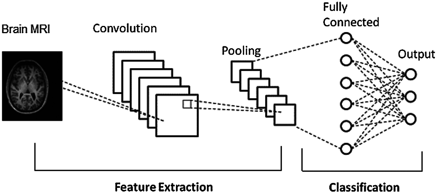
Figure 1: CNN architecture

In this section, the key components of the Histogram and Time-frequency Differential Deep (HTF-DD) method for Medical Image Classification are highlighted, providing a description of the coding network and the medical image pre-processing in Subsections 3.1 and medical image feature extraction in 3.2. In Subsection 3.3, the actual medical image classification is detailed.

Fig. 2 shows the detailed procedure of the proposed HTF-DD method which involves three different steps. In the first step, Histogram Intensity-oriented Pre-processing model is applied in the convolutional layer where pooled feature mapping is performed with the histogram function, therefore generating pooled feature maps (i.e., standardized intensified pre-processed features). Next, in the second step, time and frequency are applied in the pooling and fully connected layers, therefore extracting time-frequency maps (i.e., optimal time-frequency feature extraction). Finally, softmax function is applied to the sample features to obtain discrete probable distribution, which characterizes the probable results of a random variable that can take on one of ‘n’ possible classes, with the probability of each class separately specified.

3.1 Histogram Intensity-Oriented Pre-Processing Model

In the present study, the classification of medical images for Brain MRI images is taken into consideration. Though several researches have been conducted using these types of images, the main issue to be addressed while classifying these types of images is the intensity that differs even for the same protocol, body region, patient and scanner.

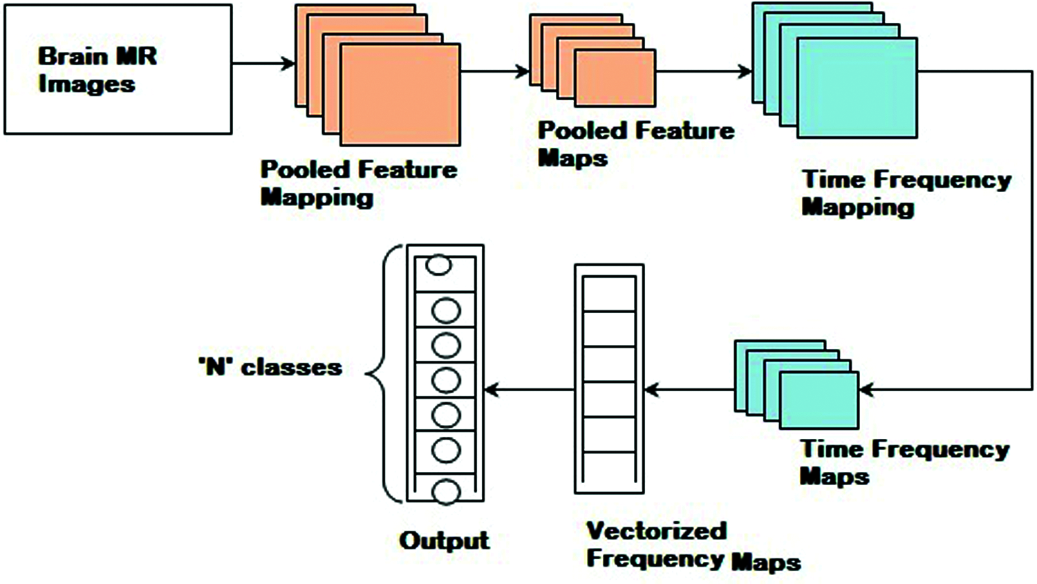
Figure 2: Block diagram of histogram and time-frequency differential deep (HTF-DD) method

In this work, intensity is concentrated during the pre-processing stage itself, therefore reducing the error rate (i.e., improving PSNR) involved in pre-processing. These Brain MR images are initially said to be standardized by means of histogram. The pseudo code representation of Histogram Intensity-oriented Pre-processing is given as Algorithm 1.

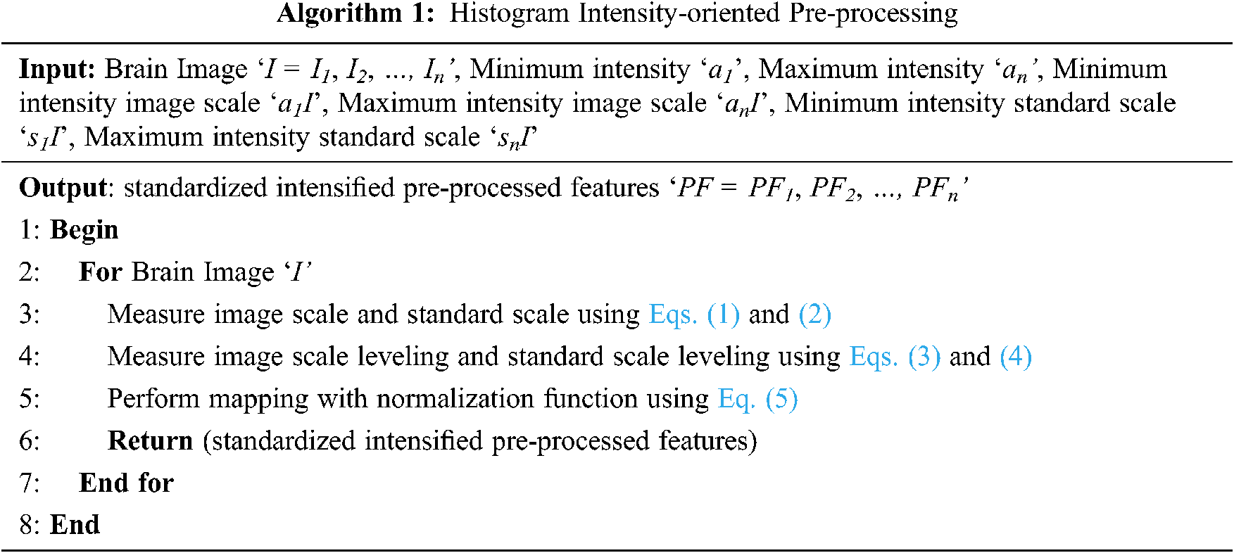
With the above supposition, for a given brain image ‘I’, minimum intensity image scale, maximum intensity image scale, minimum intensity standard scale and maximum intensity standard scale and standard scale values are obtained by means of histogram. Then the image scale ‘IS’ and standard scale ‘SS’ are represented as given below in Eqs. (1) & (2).

IS=a1I,…,s1I,…,μi,…,s2I,…,anI (1)

SS=s1I,…,s1,…,μs,…,s2,…,snI (2)

Then from the above equations, leveling is said to be performed between ‘IS’ and ‘SS’. The image scale leveling ‘ISL’ and standard scale leveling ‘SSL’ is mathematically formulated as given below as Eqs. (3) and (4).

ISL={μI−a1I,μI−a2I,…,μI−anI} (3)

SSL={μs−s1,μs−s2,…,μs−sn} (4)

Finally, with these two equations, the standardized pre-processed features ‘PF’ with optimal intensity are obtained as given below in Eq. (5) using the two conditions.

PF={b[s1−μsa1I−μI]b[s2−μsa2I−μI],ifa1I≤b≤μIandμI≤b≤anI (5)

With the above standardized pre-processed features ‘PF’, the next section concentrates on the feature extraction for medical brain image classification.

3.2 Medical Time-Frequency Feature Extraction

With the obtained pre-processed images, the part that is considered to be the most important for medical image classification is feature extraction. Feature extraction refers to the utilization of a machine to extract vital portion of images and determine its priority. The objective behind feature extraction therefore remains in partitioning the image points into several subsets. Different types of features are present in the image and based on several criteria, classifications will be made. The global or local features are said to persist based on the feature size. As several researches have been conducted using local or global features, in the present study, time-frequency algorithm is used for feature extraction to achieve faster training and testing which is shown in Fig. 3.

The time-frequency algorithm for brain MRI images involves a concurrent processing model. Due to this, the feature extraction is said to achieve faster training and testing. Based on the feature extraction of target image in time domain and frequency domain, the depth extraction technique with standardized intensified pre-processed features ‘PF’ extracts the target information from brain MRI images. To start with, time-frequency signal models for multiple standardized intensified pre-processed features of brain MRI images are created with the following Eqs. (6) and (7).

g(PF)=Sf(PF−τ) (6)

S=([ISL−SSL]/[ISL−SSL][ISL+SSL][ISL+SSL]) (7)

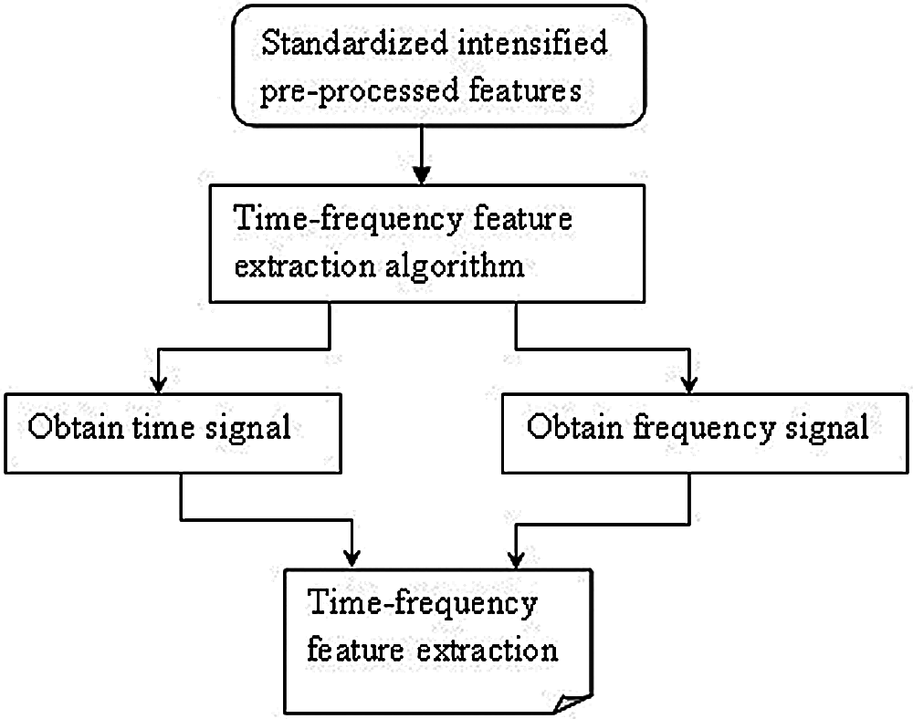
Figure 3: Block diagram of medical time-frequency feature extraction

From the previous equations, ‘S’ refers to the original pre-processed feature signal, called the image scale factor, with the size of the feature signal being ‘s’ and ‘S(i, j)’, representing the ‘ith row’, ‘jth column’ element in ‘S’ respectively. Referred to as scale, it represents the signal scaling change in the original image time-frequency feature extraction algorithm. ‘√S’ is the normalized factor of image time-frequency feature extraction algorithm. Next, the one-dimensional function is mapped to the two-dimensional function ‘b(t)’ of the time proportion ‘i’ and the time conversion ‘j’. The time-frequency transformation on the pre-processed brain MRI image using the quadrangle function is carried out as given below in Eq. (8).

Wφb(i,j)≤b,φij≥∫−∞+∞b(t)1iφ(t−ji)dt (8)

From the above equation, ‘ψij’ is ‘ψ (t)’ obtained by transforming ‘U (i ,j)’ via the affine group as given below in Eq. (9).

φij(t)=[ U(i,j)φ(t) ]= 1iφ(t−ji) (9)

Finally, by substituting the variable of the pre-processed brain MRI image ‘f (PF)’ by ‘i = 1/s’ and j = τ’, the above equation is re-written as given in Eq. (10).

fs,τ(t)=[U(1s,τ)f(t)=Sf(t[PF−τ])] (10)

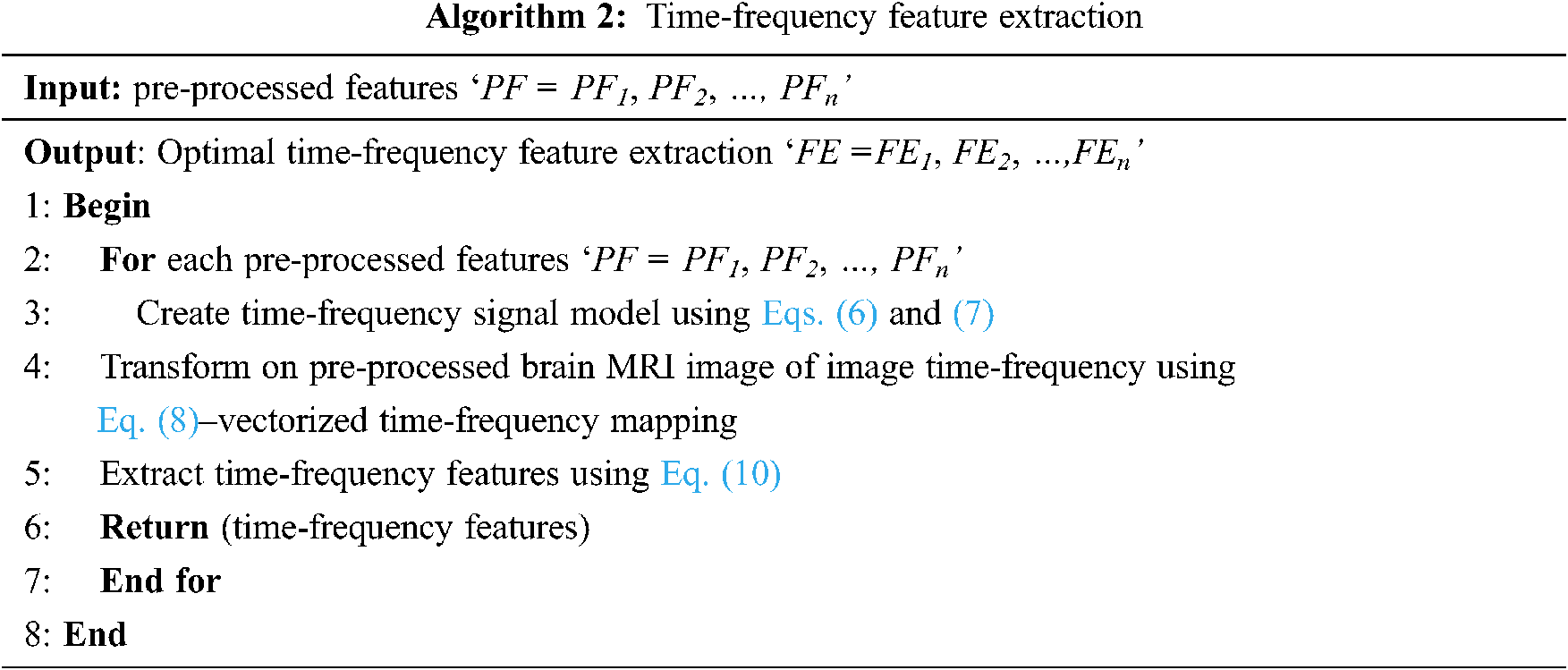
From Eq. (10), the less complex time-frequency features are extracted in a significant manner. With these, time-frequency features are extracted, and finally, the brain MR images are classified using differential deep image classification. The pseudo code representation of time-frequency feature extraction is given below as Algorithm 2.

3.3 Differential Deep Medical Image Classification

Finally, a softmax function is used in the current study to classify ‘n’ different classes via measuring the probability of belonging to each class. The softmax function is being utilized as the activation function in output layer of CNN and it regularize the output of a network to forecast the probability distribution. When compared with the sigmoid and ReLU [1], though the sigmoid functions are said to be applied in an easy manner, despite, dealing with medical image classification, only two classes are said to be obtained using the sigmoid function. Besides this, with ReLU, there is a positive bias in the network as the mean activation is greater than zero. Though the application of ReLU is said to be computationally efficient, the positive mean shift slows down learning. However, by applying the softmax function, a large number of classes are said to be formed, squashing the outputs of each unit between 0 and 1. The softmax function includes a sample vector and weight vector. The sample vector is represented as ‘FE’ and the weighted vector is represented as ‘θT’ and the function is mathematically expressed as given below from Eqs. (11)–(15).

Δw=∂∂w[12(f(a)−b)2] (11)

=12[2∗(f(a)−b)∗∂∂w(f(a)−b)] (12)

=(f(a)−b)∗∂∂w(f(a)) (13)

=(f(a)−b)∗∂∂w(11+e−(wx+b)) (14)

=f(a)−b)∗f(a)∗(1−f(a)∗a) (15)

Prob(b=j|a,θ)=eΔw(FE)∑j=1n⁡eΔw(FE) (16)

From the above equation, the sample vector in the present study represents the feature extracted from the above section using time-frequency model and the weight vector is the differential result obtained from Eq. (16). The pseudo code representation of Differential Deep Image Classification is mentioned below in Algorithm 3.

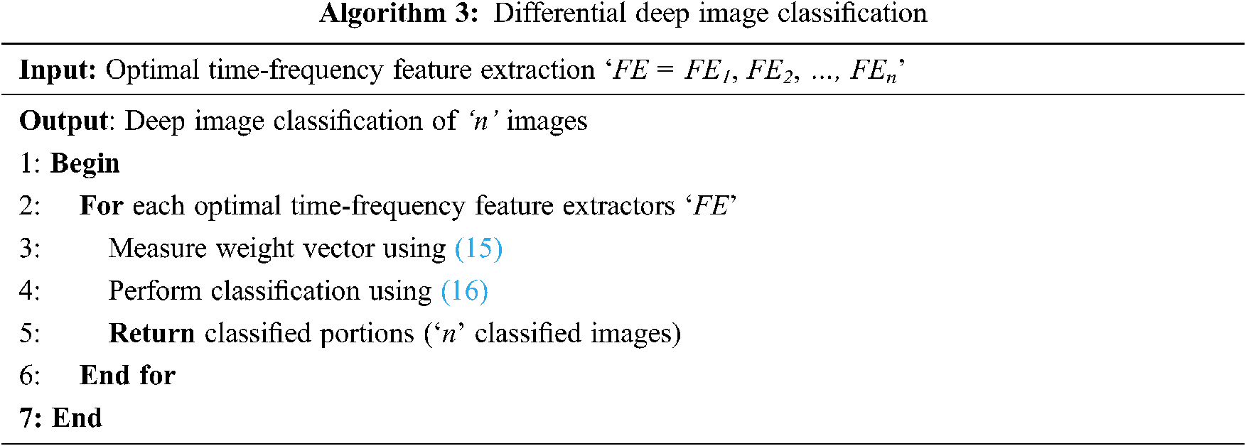
As given in Algorithm 3, for each sample vector image (i.e., time-frequency feature extractors), a weight vector is obtained. The weight vector is evaluated by means of differential function. The purpose of using the differential function is, that, as far as brain MRI is concerned, continuous changes are said to be observed at different time intervals. The process of applying differential equations in image classification helps to relate a vector of its independent variables, therefore improving the convergence speed.

4  Experimental Settings and Results

Brain medical image classification with MRI images is implemented using matlab toolbox that implements CNN as well as extracts the time-frequency features. A series of experiments have been designed to verify the effectiveness of HTF-DD method using NBIA Brain MRI images. To measure the performance, three parameters are tested; computational complexity, computational overhead and classification accuracy metrics. All the three experiments are conducted on a computer with i5-6500 3.2 GHz CPU, 32 G main memory and GTX1060 GPU. The two state-of-the-art works like convolutional neural network based approach [a] and Kernel Learning method [b] are used for comparison.

4.1 Evaluation Measures

To evaluate the proposed HTF-DD method, three metrics that are commonly used in the literature are selected. The computational complexity, computational time and classification accuracy parameters are analyzed, which shows the performance of brain medical image classification. According to the objective of HTF-DD method, i.e., to classify the brain medical image with higher accuracy with less time and overhead, evaluation metrics are chosen. These metrics are computed with respect to the number of images and the results are given Tabs. 2–4.

4.2 Dataset

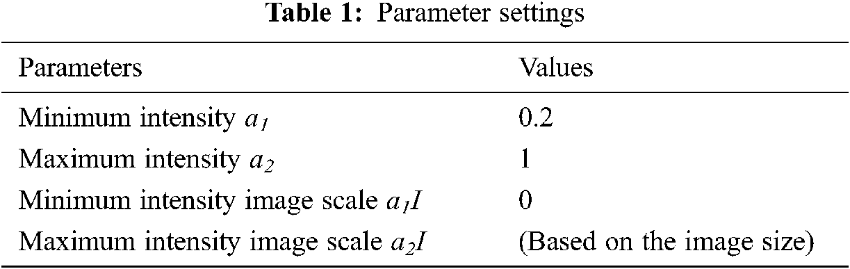
NBIA comprises a searchable repository of vivo images that ensure the biomedical research persons, industrial experts and academic profession to extract image archives to be utilized in the area of development and validation of medical image classification. This is highly suitable for detecting lesion, classifying the images, diagnosis, quantitative assessment, providing feedback and so on. The parameter settings have the intensity values in the range of 0.2 to 1 which is tabulated in Tab. 1. The sample brain images also are given below in Fig. 4.

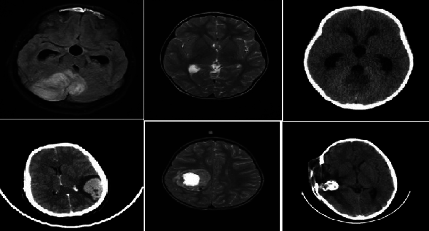
Figure 4: Sample brain tumor images

The parameter settings of the proposed algorithm are shown in Tab. 1.

4.3 Computational Complexity

Classification of medical images is of paramount importance for the success of disease diagnosis. Computational complexity refers to the complexity involved in computing the classification process. The lower the complexity, the more efficient the method is said to be and it is expressed in Eq. (17).

CC=∑i=1n⁡Ii∗MEM(IC) (17)

In the above equation, the computational complexity ‘CC’ is measured based on the number of brain MR images considered for experimentation ‘Ii’ and the memory consumed in image classification ‘MEM(IC)’. The computational complexity is measured in terms of Kilobytes (KB). The results are tabulated in Tab. 2.

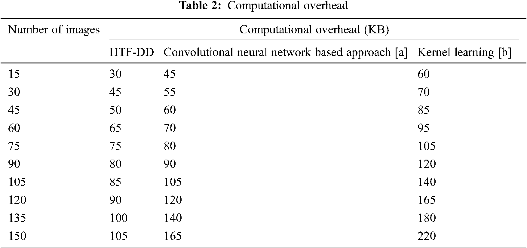
From the calculation shown in Tab. 2, with ‘15’ numbers of images used for experimentation, the computational complexity using HTF-DD is found to be ‘30 KB’ the computational complexity using convolution neural network based approach [a] is found to be ’45’ and ’60 KB’ using Kernel Learning [b]. The improvement in complexity using HTF-DD method is due to the incorporation of time-frequency feature extraction model. By applying both the time and frequency for extracting the features, faster training and testing are said to be achieved by means of vectorized time-frequency mapping. With this, optimal time-frequency features are extracted, therefore minimizing the complexity incurred in classification using HTF-DD method by 20% compared to [a] and 40% compared to [b].

4.4 Computational Time

The second most important metric for Brain MR medical image classification is the time involved in classification. This is because with the minimum time incurred in classification, the convergence speed is faster and maximum numbers of images are found to be classified and so the computational time is lower. The computational time is measured as given below in Eq. (18).

CT=∑i=1n⁡Ii∗Time(IC) (18)

From Eq. (18), the computational time ‘CT’ is measured based on the number of brain MR images considered for experimentation ‘Ii’ and the time consumed in image classification ‘Time(IC)’. The computational time is measured in terms of milliseconds (ms) which are tabulated in Tab. 3.

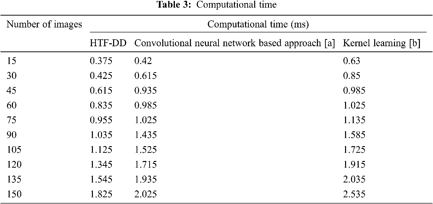
From the table, it is inferred that the number of images is directly proportional to the computational time. This is because of the reason that with the increase in the number of images, the image size increases and obviously, the computational time involved in the classification of images also increases. This is evident from the sample calculation where the computational time for classifying a single image being ‘0.025 n’ using HTF-DD method, the computational time for classifying single using [a] is found to be ‘0.028 n’ and ‘0.042 n’ by applying Kernel Learning. Therefore the overall classification time using the HTF-DD method is found to be ‘0.25 n’, ‘0.42 n’ and ‘0.63 n’ using the existing methods. This is because of the application of Histogram Intensity-oriented Pre-processing algorithm where standardized intensified pre-processed features are obtained by means of mapping image scale leveling and standard scale leveling using a normalization function. Moreover, for extracting the features based on time and frequency, the computational time using HTF-DD method is found to be reduced by 20% compared to [a] and 31% compared to [b].

4.5 Classification Accuracy

Finally, the classification accuracy or the accuracy rate with which the medical images is being classified is measured. The higher the classification accuracy, the more efficient the method is said to be. In other words, the classification accuracy refers to the percentage ratio of medical images correctly classified to the overall sample images considered for experimentation. It is mathematically expressed in the Eq. (19).

CA=Icc∗100I (19)

From Eq. (19), the classification accuracy ‘CA’ is measured according to the sample images provided as input ‘I’ and the number of images correctly classified ‘ICC’. The classification accuracy is measured in terms of percentage (%) and the results are shown in Tab. 4 and Fig. 5.

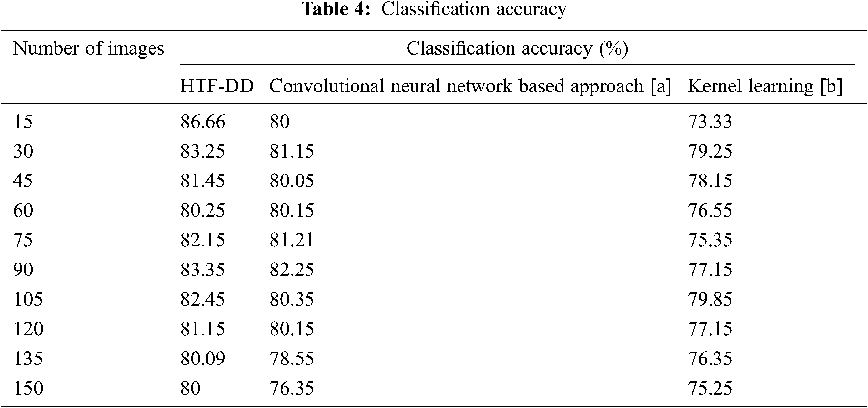
Fig. 5 illustrates the graphical representation of classification accuracy with respect to 150 different numbers of images. With the increase in the number of images, the classification accuracy gets reduced. Therefore the number of images is inversely proportional to the classification accuracy. From this, it is inferred that the classification accuracy is found to be improved by applying the HTF-DD method. This is because of the incorporation of DD classification algorithm. By applying this algorithm, two significant things are said to happen. At first, vectors are considered; one sample vector and weight vector. In the sample vector, the optimal features with standardized intensified pre-processed features are used. Next, in the weight vector, a differential function is applied so that independent variables, irrespective of time, are considered.

With these two factors, the classification is said to be performed in an efficient manner. Therefore the classification accuracy using HTF-DD method is found to be better by 3% compared to [a] and 7% compared to [b].

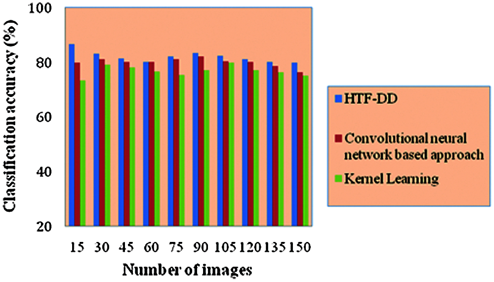
Figure 5: Performance graph of classification accuracy

This accuracy results have been compared with previous works in [18] where CNN models like AlexNet, ResNet-50 were implemented for lymph node images classification. The accuracy obtained using sequential gaussian simulation in implementing AlexNet for 138 malignant lymph node images is 57.14% and for 133 benign images is 78.57%. Brain tumor and survival prediction are experimented with benchmark dataset and achieved 61.0% of accuracy in [28]. While comparing these results, out research work performs well in terms of classification accuracy. Also, the computational time needed for classification in our research work is about 3.7 × 10−4 s for 15 images whereas in [21] the time needed is 15 × 10−4 s for 15 images. As mentioned in literature review, lot of methodologies with machine learning and deep learning algorithms exists. But it is relatively difficult to compare all the models with different datasets. Since, most of the methodologies reported accuracy and loss as the result, the same has been taken for comparison.

5  Conclusion

In this paper, a novel Brain MR Image classification method that integrates time-frequency feature extraction from a Histogram Intensity Pre-processing network and classifies it via Differential Deep Learning is presented. It is named as Histogram and Time-frequency Differential Deep (HTF-DD) method. The proposed method is analyzed in terms of complexity and accuracy. To reduce the complexity involved in the classification of medical images, Histogram Intensity-oriented pre-processing is applied at first. Next, feature extraction is performed for the pre-processed features by applying the time and frequency factors. With these two processes, the complexity involved in classification is reduced. Finally, with the optimal pre-processed features, a deep learning model based on differential factor is applied to classify the images into different classes. With this, the classification accuracy is said to be enhanced as 80% for 150 images. A sufficient improvement in computational complexity and classification accuracy is also seen from the experimental results. Although this research work HTF-DD approach performs well when compared to conventional CNN and Kernal methods, it has to be evaluated with other deep learning architectures to show its aggressive advantage.

Acknowledgement: We thank the anonymous referees for their useful suggestions.

Funding Statement: The authors received no specific funding for this study.

Conflicts of Interest: The authors declare that they have no interest to report regarding the present study.

This work is licensed under a Creative Commons Attribution 4.0 International License, which permits unrestricted use, distribution, and reproduction in any medium, provided the original work is properly cited.