Computer Systems Science & Engineering DOI:10.32604/csse.2022.020835
Article

Graphics Evolutionary Computations in Higher Order Parametric Bezier Curves

Monday Eze1,*, Charles Okunbor2, Deborah Aleburu3, Olubukola Adekola1, Ibrahim Ramon4, Nneka Richard-Nnabu5, Oghenetega Avwokuruaye6, Abisola Olayiwola3, Rume Yoro7 and Esomu Solomon8

1Department of Computer Science, Babcock University, Ogun, Nigeria
2Department of Computer Science, Admiralty University, Delta, Nigeria
3Department of Computer Science, Caleb University, Imota, Lagos, Nigeria
4Department of Computer Science Education, Federal College of Education (Tech), Akoka, Lagos, Nigeria
5Department of Computer Science, Alex Ekwueme Federal University, Ebonyi, Nigeria
6Department of Cyber Security, Admiralty University, Delta, Nigeria
7Department of Computer Science, School of ICT, Delta State Polytechnic, Ogwashi-Uku, Delta, Nigeria
8Department of Computer Science, National Open University, Nigeria
*Corresponding Author: Monday Eze. Email: ezem@babcock.edu.ng
Received: 10 June 2021; Accepted: 14 July 2021

Abstract: This work demonstrates in practical terms the evolutionary concepts and computational applications of Parametric Curves. Specific cases were drawn from higher order parametric Bezier curves of degrees 2 and above. Bezier curves find real life applications in diverse areas of Engineering and Computer Science, such as computer graphics, robotics, animations, virtual reality, among others. Some of the evolutionary issues explored in this work are in the areas of parametric equations derivations, proof of related theorems, first and second order calculus related computations, among others. A Practical case is demonstrated using a graphical design, physical hand sketching, and programmatic implementation of two opposite-faced handless cups, all evolved using quadratic Bezier curves. The actual drawing was realized using web graphics canvas programming based on HTML 5 and JavaScript. This work will no doubt find relevance in computational researches in the areas of graphics, web programming, automated theorem proofs, robotic motions, among others.

Keywords: Parametric curve; computer graphics; bezier curve; blending function; robotics

1  Introduction

The importance of parametric curves in Computer Graphics [1], Computer Aided Design (CAD), Animation, Robotics and a number of other areas of computing cannot be overemphasized. The focus of this research is on a special parametric curve known as Bezier Curves [2]. The concept of Bezier Curves originated from the works of Pirerre Biezier [3] who is renowned to have applied it in design of car chassis. A Bezier curve is a smooth parametric curve, controlled by the shape of a defining polygon. The defining polygon consists of a number of points, known as control points [4], which make up an enclosure called Convex Hall [5]. The order of a Bezier curve is equivalent to the number of control points.

For a Bezier Curve of control points P0, P1, … PN, the points P0 and PN are called end points, and the rest of the points from P1 to PN − 1 may lie outside the curve. Given that a Bezier curve is of order X, then its degree is defined as X − 1. For instance, a quadratic Bezier curve is of degree two, a cubic Bezier curve is of degree three, while a quartic Bezier curve is of degree four respectively. Computations involving Bezier curves of higher degree are said to be very expensive [6], thus, many researches tend to be limited to quadratic and cubit curves. The concept of degree elevation [7] has to do with the conversion of a Bezier curve of degree X to an entirely new one of degree X + 1 with the same shape. The De Casteljau’s algorithm [8] is one of the recursive techniques used for Bernstein polynomial evaluations.

Recent advances in Bezier curves have witnessed its applications in robotics, especially in the area of path planning and generation [9]. Engineering researches in the area of multi-material flow [10] make use of the parametric curves. The Bezier parametric curves are also utilized in creating aesthetic automobile surfaces and in evaluating reflected images in ocean research [11]. Among other applications, some of the most common are in Computer Graphics, Animation [12], and Virtual reality [13]. These and many other real-life applications of Bezier curves make adequate use of the foundational concepts. Thus, this work demystifies evolutionary concepts that touch on theorems, proofs, algorithms, and computations in parametric Bezier curves relevant to computer graphics.

This work is organized into ten sections. First is an introduction, and then a computational exploration of parametric functions. This is followed by studies on blending function derivations, Bezier matrix, Bezier curve sketching, curve join and foundational proofs of two important theorems. The concluding part of this work focused on derivatives, system implementations, and a conclusion.

2  Parametric Exploration

The general parametric equation of a Bezier curve is given by Eq. (1).

Z(x)=∑k=0nPkJN,k(x),0≪x≪1 (1)

where, Z(x) is any point on the curve, Pk is the kth Control point of the Bezier Curve, JN,K(x) is the Bernstein or Blending function, N is the degree of the Bezier Curve in question. The Blending function is the control function, also referred to in a of number previous researches as the Bezier basis functions. The components of Z(x) are further defined as follows:

JN,k(x)=CkNxk(1−x)N−k (2)

CkN=N!k!(N−1)! (3)

N!=(1).(2).(3)…N (4)

It can be deduced from the “Eqs. (1)–(4)” that the Parametric equation Z(x) is the sum of the products of Blending functions J and the corresponding control points P.

3  Blending Function Derivation

It is necessary at this stage to demonstrate the derivation of higher order blending functions. A 5th order will be used as a case study.

Given a Bezier Curve of 5th Order, one important task is to derive all the blending functions [14]. Since the Order of a Bezier Curve is same as the number of control points, it implies that a Bezier curve of 5th order has a total of five (5) control points. The relationship between the Order and the Degree of a curve is given by Eq. (5):

Degree=Order−1 (5)

Thus, for a 5th order case, the degree is N = 5 – 1, which is 4. The Blending functions are therefore computed as follows:

JN,k(x)=CkNxk(1−x)N−k=N!k!(N−1)!xk(1−x)N−k

J4,0(x)=C04x0(1−x)4−0=4!0!(4−0)!x0(1−x)4−0

Therefore,

J4,0(x)=4!0! 4!x0(1−x)4−0=(1−x)4 (6)

J4,1(x)=C14x1(1−x)4−1=4!1!(4−1)!x1(1−x)4−1

Therefore,

J4,1(x)=4!1! 3!x1(1−x)3=4x(1−x)3 (7)

J4,2(x)=C24x2(1−x)4−2=4!2!(4−2)!x2(1−x)4−2

Therefore:

J4,2(x)=4!2! 2!x2(1−x)2=6x2(1−x)2 (8)

J4,3(x)=C34x3(1−x)4−3=4!3!(4−3)!x3(1−x)4−3

Therefore:

J4,3(x)=4!3! 1!x3(1−x)1=4x3(1−x) (9)

J4,4(x)=C44x4(1−x)4−4=4!4!(4−4)!x4(1−x)4−4

Therefore:

J4,4(x)=4!4! 0!x4(1−x)0=x4 (10)

Substituting all the Blending Functions into the general Eq. (1), the exact Parametric equation for a 4-degree Bezier Curve is therefore given by:

Z(x)=P0J4,0(x)+P1J4,1(x)+P2J4,2(x)+P3J4,3(x)+P4J4,4(x) (11)

Therefore,

Z(x)=P0(1−x)4+P14x(1−x)3+P26x2(1−x)2+P34x3(1−x)+P4x4 (12)

4  Derivation of Bezier Matrix

The Bezier Matrix derivation will be demonstrated using a 4th degree case. First, the Blending functions are written in full polynomial format, and then converted to twisted coefficient formats as follows:

J4,0(x)=(1−x)4=(1−x)(1−x)(1−x)(1−x)=(1−2x+x2)(1−2x+x2)

=1−4x+6x2−4x3+x4

In twisted coefficient format, this gives

J4,0(x)=x4−4x3+6x2−4x+1 (13)

J4,1(x)=4x(1−x)3=4x(1−x)(1−2x+x2)=4x(1−2x+x2−x+2x2−x3)

=4x(1−3x+3x2−x3)=4x−12x2+12x3−4x4

In twisted coefficient format, this gives:

J4,1(x)=−4x4+12x3−12x2+4x+0 (14)

J4,2(x)=6x2(1−x)2=6x2(1−2x+x2)=6x2−12x3+6x4

In twisted coefficient format, this gives:

J4,2(x)=6x4−12x3+6x2+0x+0 (15)

J4,3(x)=4x3(1−x)=4x3−4x4

In twisted coefficient format, this gives:

J4,3(x)=−4x4+4x3+0x2+0x+0 (16)

J4,4(x)=x4

In twisted coefficient format, this gives:

J4,4(x)=x4+0x3+0x2+0x+0 (17)

The Bezier Matrix (BEZMAT) is generated by collating all the twisted coefficients of the Blending Functions as shown in Fig. 1:

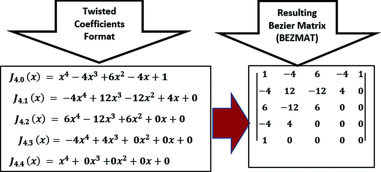
Figure 1: Sample of generated bezier matrix

Thus, the Parametric Equation in Bezier Matrix format is given by:

P(x)=[x4x3x2x1].BEZMAT.[P0P1P2P3P4] (18)

where, BEZMAT is the Bezier Matrix.

5  Bezier Curve Sketching

Suppose a Bezier Curve has four Control Points given by B0 [1, 1], B1 [4, 4], B2 [7, 3] and B3 [6, 1]. The first computational task is to determine six points lying in the curve. The second task is to sketch the curve. Since there are four control points, it implies that the curve is of Order = 4, and thus, of Degree = 3, which is a Cubic Bezier Curve. The Parametric Equation is given by:

Z(k)=B0(1−k)3+B13k(1−k)2+B23k2(1−k)+B3k3 (19)

To determine the points lying on the curve, first we select six random points (RANPO) which satisfy the inclusion condition 0 << k << 1.

LetRANPO=[0,0.2,0.4,0.5,0.8,1.0] (20)

Substituting the values of the Control Points B0, B1, B2, B3 and B4 in the Parametric equation, we have:

Z(k)=[11](1−k)3+[44]3k(1−k)3+[73]3k2(1−k)2+[61]k3 (21)

For Parameter k = 0:

Z(0)=[11](1−0)3+[44]3(0)(1−0)2+[73]3(0)2(1−0)+[61](0)3=[1.01.0]

For Parameter k = 0.2:

Z(0.2)=[11](1−0.2)3+[44]3(0.2)(1−0.2)2+[73]3(0.2)2(1−0.2)+[61](0.2)3

=[11](0.512)+[44](0.384)+[73](0.096)+[61](0.008)

=[0.5120.512]+[1.5361.536]+[0.6720.288]+[0.0480.008]=[2.7682.344]

For Parameter k = 0.4

Z(0.4)=[11](1−0.4)3+[44]3(0.4)(1−0.4)2+[73]3(0.4)2(1−0.4)+[61](0.4)3

=[11](0.216)+[44](0.432)+[73](0.288)+[61](0.064)

=[0.2160.216]+[1.7281.728]+[2.0160.864]+[0.3840.064]=[4.3442.872]

For Parameter k = 0.5

Z(0.5)=[11](1−0.5)3+[44]3(0.5)(1−0.5)2+[73]3(0.5)2(1−0.5)+[61](0.5)3

=[11](0.125)+[44](0.375)+[73](0.375)+[61](0.125)

=[0.1250.125]+[1.5001.500]+[2.6251.125]+[0.7500.125]=[5.0002.875]

For Parameter k = 0.8

Z(0.8)=[11](1−0.8)3+[44]3(0.8)(1−0.8)2+[73]3(0.8)2(1−0.8)+[61](0.8)3

=[11](0.008)+[44](0.096)+[73](0.384)+[61](0.512)

=[0.0080.008]+[0.3840.384]+[2.6881.152]+[3.0720.512]=[6.1522.056]

For Parameter k = 1.0

Z(1.0)=[11](1−1)3+[44]3(1)(1−1)2+[73]3(1)2(1−1)+[61](1)3

=[11](0.0)+[44](0.0)+[73](0.0)+[61](1.0)=[61]

The sketch of the curve is shown in Fig. 2. The control points are B0, B1, B2, and B3. The curve is shown in red colour, and the six points estimated to lie on the curve are E0, E1, E2, E3, E4 and E5. The enclosure B0 B1 B2 B3 B0 constitutes the convex hall.

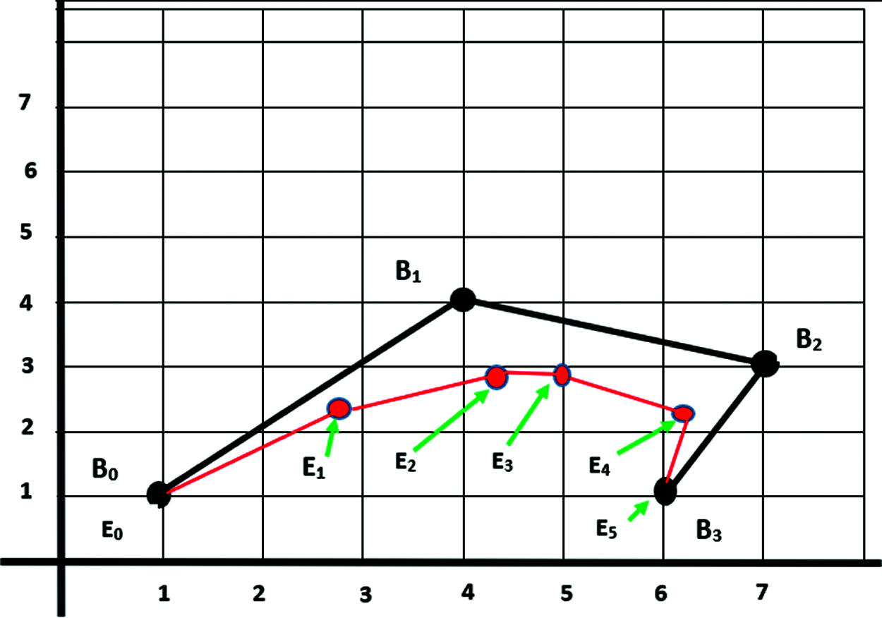
Figure 2: A sample cubic bezier curve

6  Curve Join Condition

In a number of scientific applications, there are cases where two or more parametric curves need to be joined to form a single one. This process is tagged curve continuity [15]. Imagine two separate Bezier Curves P and Q shown in the left-hand side (LHS) of Fig. 3, with P0 and Q0 as starting points of the curves, and P1 and Q1 as the end points respectively. The two separate curves are joined to form a single curve shown in the right-hand side (RHS) of the figure.

For curve continuity to hold, some computational conditions must be met. These are known as zero-order, first order, and third order parametric continuities respectively as will be discussed next.

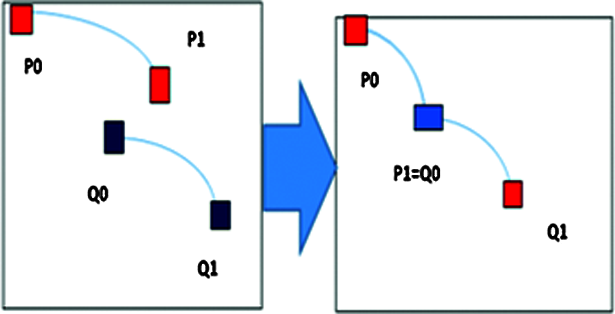
Figure 3: Demonstration of curve joining

First and foremost, for any two curves to P and Q to be joined, such that P is followed by Q, then the end point of curve P must be the beginning point of curve Q. This is known as the zero-order parametric continuity condition [16] as demonstrated in the RHS of Fig. 3. The equation is given by

P(1)=Q(0) (22)

Secondly, suppose the two curves P and Q are of degree N, then for the join to be smooth, the first-order parametric condition must hold. The conditional equation is a derivative [17] given by:

P1(1)=Q1(0) (23)

Thus, the first-order parametric continuity condition [18] ensures the smoothness of a joint curve. The implication of this rule is that the tangent at the end point of first curve P is the same as the tangent at the first point of the second curve Q. As earlier proved in this research, the first derivatives of P at end points are given by the equations:

P1(0)=n(P1−P0) (24)

P1(1)=n(PN−PN−1) (25)

Finally, second order parametric continuity condition [19] states that second derivates at the end point of the first curve P is the same as that of the beginning point of second curve Q. Mathematically:

PII(1)=QII(0) (26)

Again, the formula for the second derivatives at the beginning and end points are given by:

PII(0)=N(N−1)(P2−2P1+P0) (27)

PII(1)=N(N−1)(PN−2PN−1+PN−2) (28)

Research has shown that whenever a curve satisfies the second order parametric continuity, it also automatically satisfies the first order continuity [20].

7  Foundational Proofs

A number of foundational theorems of Bezier Curves are of key applications to Computer Graphics. Two of these theorems to be proved in this work are the partition of unity theorem and the symmetry theorem respectively.

7.1 Partition of Unity Theorem

The partition of unity theorem [21] states that the sum of the Bernstein Polynomial of degree N is equal to unity. Mathematically:

∑k=0NBk,N(t)=1,wheret∈[0,1] (29)

Proof:

Obviously, the trivial statement [(1 − t) + t] = 1 is always true for every parameter t. Substituting this statement into a general Binomial Eq. (29), we have:

1=(1)N=[(1−t)+t)N=∑k=0N[Nk](1−t)N−k(t)k=∑k=0NBk,N(t)

which completes the proof.

7.2 Bernstein Symmetry Theorem

The Bernstein Symmetry Theorem [22] states that every Berstein Polynomial follows the mathematical symmetry as follows:

BN−k,N(x)=Bk,N(1−x) for k∈[0,1] (30)

Expanding the LHS of the symmetry Eq. (30) gives:

BN−k,N(x)=N!(N−(N−k))!(N−k)!(1−x)(N−(N−k))xN−k

Therefore,

BN−k,N(x)=N!k!(N−k)!(1−x)kxN−k (31)

Expanding the RHS of the symmetry Eq. (30) gives:

Bk,N(1−x)=N!(N−k)! k!(1−(1−x))N−k(1−x)k

Therefore,

Bk,N(1−x)=N!(N−k)! k!xN−k(1−x)k (32)

By simple comparison, it is clear that “Eqs. (31) and (32)” are same. Thus, the theorem is proved.

8  Derivation of Derivatives

Derivatives of parametric curves is of key importance, due to its application in Computer Graphics and other areas of computing. Research has shown that the derivative of Bezier Curve is also in itself, another Bezier curve [23]. An unambiguous demonstration of the derivation process beginning with product rule of Calculus is as follows:

ddxBk,N(x)=N!(N−k)! k!ddx(1−x)N−k(x)k (33)

=N!(N−k)! k!(−(N−k)(1−x)N−k−1(x)k+(1−x)N−k.k.xk−1

=−(N−k)N!(N−k)! k!(1−x)N−k−1(x)k+N!k(N−k)!k!(1−x)N−k.xk−1

 =−N(N−1)!(N−k−1)!k!(1−x)N−1−k(x)k+N(N−1)!(((N−1)−(k−1))!(k−1)!)!(1−x)(N−1)−(k−1).xk−1

=−N(Bk,N−1(x))+N(Bk−1,N−1(x))

Therefore,

ddxBk,N(x)=N(Bk−1,N−1(x)−Bk,N−1(x)) (34)

which is the formula for first derivative.

9  System Implementation

Before concluding this work, it is necessary to demonstrate the generation of Bezier Curves and applications in computer graphics in programmatic terms. A number of programming languages have application programming interface (API) or re-usable modules [24] specifically available for Bezier Curves related graphical designs and implementations. For instance, in Python the Bezier module is installed using the command pip install Bezier [25], and can be invoked into the programming environment using the command import Bezier [26].

However, Python versions 3.7 to 3.8 may bring “DLL Load Failed while importing _Speedup” error message in attempt to import Bezier as shown in Fig. 4, especially due to failure in pip installation process.

This anomaly is common in a number of Python integrated development environment (IDEs) such as Spider, Jupyter and Pycham used within Anaconda [27].

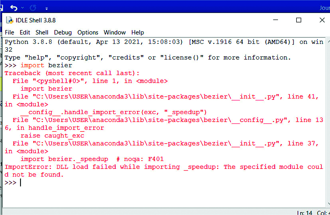
Figure 4: Load failed error message in python

One very feasible alternative is the use of Canvas tools [28] in web graphics. The hypertext markup language (HTML) canvas can be used in conjunction with JavaScript [29] to build complex graphical objects in a bottom-up approach, beginning from simple parametric Bezier curves as components. The canvas element is a graphical container, which is driven by Javascripts to generate graphical kernels such as paths, boxes, circles, text, images, images, and many others.

By its nature, a canvas is borderless and empty until it is enabled with Javascript. This is achieved by specifying an <id attribute> tag to refer it in a script. Furthermore, the width and height attributes are used to define the size of the canvas, and then the style attribute is used to add a border. The sample code snippet shown in Fig. 5 was saved as a HTML file called canvas.html and executed in a browser to give the output on the right-hand side.

Figure 5: Boarder drawing canvas code

The canvas functions for drawing quadratic and cubic Bezier curves are quadraticCurveTo and bezierCurveTo respectively.

The syntax for creating a quadratic Bezier is quadraticCurveTo (ctx, cty, a, b); where (ctx, cty) represent the coordinate of the control point, (a, b) is the coordinate of the end point, whereas the current point is achieved using the moveTo command.

In a similar way, since the cubic Bezier has two control points, the syntax for creating it is given by bezierCurveTo(ctx1, cty1, ctx2, cty2, a, b); where (ctx1, cty1) and (ctx2, cty2) represent the coordinates of the two control points.

The practical demonstration in this work uses HTML 5 Canvas in conjunction with Javascript for programming to implement the physical design shown in Fig. 6. The curve implementation is limited to use of quadratic Bezier curves only. The aim is to use quadratic Bezier curves to create handless twin-cups. One of the cups is standing up, while the second is turned upside down.

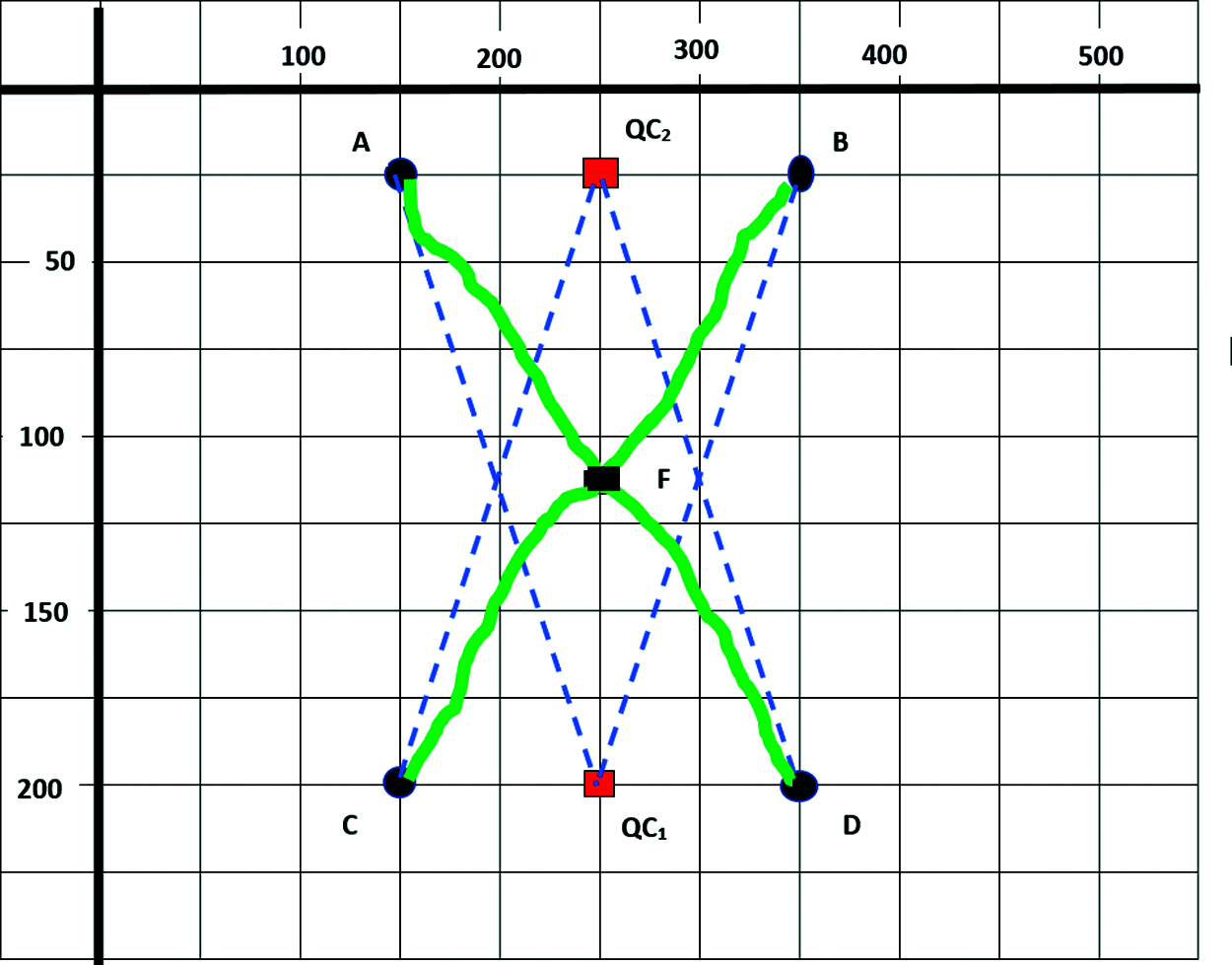
Figure 6: Physical design of bezier curves

A careful look at the diagram shows that the design space is of dimension 500 × 200. The coordinate points visibly marked are A (150, 25), B (350, 26), C (150, 200), D (350, 200), F (250, 125), QC1 (250, 200) and QC2 (250, 25).

The points QC1 and QC2 which are marked in RED colour are the control points-QC1 is the control point for the upper quadratic Bezier curve while QC2 is the control point for the lower quadratic curve. The point A and B are the end points of the upper quadratic curve, while C and D are the end points of the lower curve.

The upper cup is ABF while the lower cup turned up-side down is CFD. Both have been sketched using a handheld pencil, all of which are to be generated using Bezier curves. Both cups touch at point F. The program output is shown in Fig. 7, while the canvas program source code is shown in Section 9.1.

Figure 7: Output of program runs

9.1 Source Code

The source code is as follows:

<!DOCTYPE HTML>

<! Bezier Curve Design Sample Project. Implemented in Canvas>

<html>

<head>

<style>

body {

margin: 0px;

padding: 0px;

}

</style>

</head>

<body>

<canvas id="BezierCurveDesign" width = "500" height = "200"></canvas>

<script>

var canvas = document.getElementById('BezierCurveDesign');

var context = canvas.getContext('2d');

context.beginPath();

context.moveTo(150, 25);

context.lineTo(350, 25);

// First Quadratic curve

context.quadraticCurveTo(250, 200, 150,25);

context.moveTo(150, 200);

context.lineTo(350, 200);

// Second Quadratic curve

context.quadraticCurveTo(250, 25, 150, 200);

context.lineWidth = 10;

context.strokeStyle = 'blue';

context.stroke();

</script>

10  Conclusion

This research has presented a very unambiguous study of Bezier Parametric curves. It lays theoretical foundation of Bezier curves, and presents relevant theorems and corresponding proofs. The importance of Bezier curves in Computer Graphics, and in other fields of computing was touched. The work was concluded by showing how Bezier curves could be programmed using HTML 5 canvas and Java Script.

While Bezier parametric curves have a lot of possibilities, there are however some limitations. One limitation is the obvious computational complexity, especially for handling higher order cases [30]. This is why a number of applications tend to focus their interests on cubic and quadratic cases. Secondly, it is also difficult to get exact points on the curve. This issue however, has been resolved using a number of algorithms, for instance de Casteljau [31,32].

As a means of evaluation, it is necessary to mention other works or tools that could be comparable to the use of canvas technology, as this current study. The Open GL has been successfully explored in Bezier curves implementations in a research by [33]. However, the focus was limited to cubic cases.

A number of other comparable works are [34], which is uses Adobe Illustrator, [35] which is uses 3D Maya, based on animation techniques, both of which are mainly used for drawing the required objects. On the other hands, [36] is a computational work, though the main focus was on the control points of Bezier curves, unlike this research which covered evolutionary computational issues, as well as the programmatical implementation.

Funding Statement: The authors received no specific funding for this study.

Conflicts of Interest: The authors declare that they have no conflicts of interest to report regarding the present study.

This work is licensed under a Creative Commons Attribution 4.0 International License, which permits unrestricted use, distribution, and reproduction in any medium, provided the original work is properly cited.