Computer Systems Science & Engineering DOI:10.32604/csse.2022.020634
Article

Clustering Gene Expression Data Through Modified Agglomerative M-CURE Hierarchical Algorithm

E. Kavitha1,*, R. Tamilarasan2, N. Poonguzhali3 and M. K. Jayanthi Kannan4

1A Constituent College of Anna University, University College of Engineering, Villupuram, 605103, India
2A Constituent College of Anna University, University College of Engineering, Pattukkottai, 614701, India
3Department of Computer Science and Engineering, Manakula Vinayagar Institute of Technology, Puducherry, 605107, India
4Department of Computer Science Engineering, Faculty of Engineering and Technology, JAIN (Deemed-To-Be University), Bangalore, 562112, India
*Corresponding Author: E. Kavitha. Email: ekavitharesearch1@gmail.com
Received: 01 June 2021; Accepted: 11 July 2021

Abstract: Gene expression refers to the process in which the gene information is used in the functional gene product synthesis. They basically encode the proteins which in turn dictate the functionality of the cell. The first step in gene expression study involves the clustering usage. This is due to the reason that biological networks are very complex and the genes volume increases the comprehending challenges along with the data interpretation which itself inhibit vagueness, noise and imprecision. For a biological system to function, the essential cellular molecules must interact with its surrounding including RNA, DNA, metabolites and proteins. Clustering methods will help to expose the structures and the patterns in the original data for taking further decisions. The traditional clustering techniques involve hierarchical, model based, partitioning, density based, grid based and soft clustering methods. Though many of these methods provide a reliable output in clustering, they fail to incorporate huge data of gene expressions. Also, there are statistical issues along with choosing the right method and the choice of dissimilarity matrix when dealing with gene expression data. We propose to use a modified clustering algorithm using representatives (M-CURE) in this work which is more robust to outliers as compared to K-means clustering and also able to find clusters with size variances.

Keywords: Clustering; gene identifiers; representatives; dimension reduction

1  Introduction

As the data sets grows higher and higher, there is a need for good methods to identify the underlying patterns for effective storage and prediction purposes. One such example is dealing with high amount of gene expression data to identify biologically significant subsets of samples [1]. Tools can be used for modelling certain aspects of the biological theories. One such aspect is that a subset of genes or samples are involved in the cellular process of interest and upon receiving the stimuli, the genes of the same pathway may be suppressed or induced simultaneously. Genes with high connectivity are much lesser than genes with low connectivity. Clustering genomic data deals with high dimensional data and they are generated with the help of new technologies such as microarrays, next generation sequencing and eQTL mapping [2]. This large volume of data from microarray analysis and other clustering methods will help diagnose and treat various diseases based on gene expression profiling. All these reasons, pushes the need for identifying computational methods to process and analyse such amounts of data in depth. A classic gene expression matrix is presented in Fig. 1.

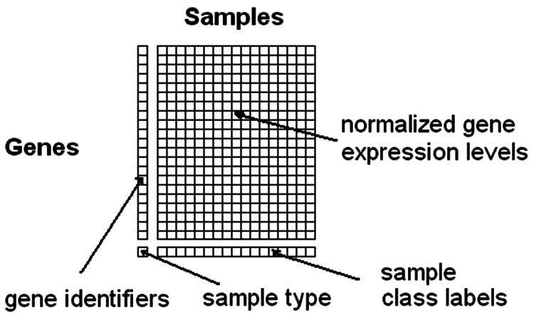
Figure 1: Gene expression matrix

The raw microarray data are converted in to gene expression matrices in which the tables with the rows will signify the genes and columns will denote different samples like tissues [3]. Hierarchical clustering is an algorithm that will help to group similar objects in to clusters. The output of the algorithm will be a cluster set where each one is different from other but the objects inside are broadly related in nature [4]. Clustering algorithms were widely applied to microarray data for years. They involve the procedure of grouping a set of nonconcrete objects in to classes of identical objects.

Consider an experimentation in which one gathers I randomly sampled objects, a J-dimensional gene expression data is represented by

Xi can represent the gene expression outline of tumour tissue comparative to normal tissue within a arbitrarily sampled patient. To see clustering as a numerical method, it is important to study Xi as an opinion of a random vector with a population spreading and we will represent it with P. These I identical and independently distributed (i.i.d.) annotations can be stored in an observed J × I data matrix X. Genes are generally characterised by I-dimensional vectors.

while the models are denoted by J-dimensional vectors Xi. The goal with this data set now would be to cluster these samples or genes. We know that a cluster is a collection of like elements in a group. Every cluster formed can be signified by a shape, either a summary portion like a cluster mean or one of the elements in it, which is called as a centroid.

Clustering process involve gene expression data analysis that involve both high-level and low-level analysis. The three main steps involved in this process are a) pre-processing of data b) designing an effective clustering algorithm with an appropriate distance measurement technique and c) database building to validate the cluster quality and further analysis. Though many problems are present in the cluster analysis and it’s a vast topic as well, we limit ourselves to micro array data clustering in this research work. Distance measurement techniques are used for finding the relationships between the different molecules of interest and the clustering algorithm chosen will use this relationship in various ways [5].

Hierarchical clustering can either be agglomerative or divisive. While agglomerative refers to bottom-up approach, they start with its own cluster before merging in pairs and moving up in hierarchy, divisive algorithms on the other hand is a top-down approach where the splits are performed recursively. The choice of the metric plays a significant role in deciding the shape of the cluster and some frequently used metrics for hierarchical clustering are Manhattan distance, Euclidean distance, Maximum distance, Squared Euclidean distance and Mahalanobis distance methods. Some commonly used criteria’s for linking two sets of observations are single linkage clustering, complete linkage clustering, unweighted average linkage clustering, weighted average linkage clustering and minimum energy clustering.

CURE (Clustering using Representatives) is one such hierarchical clustering method which overcomes the problem with the traditional hierarchical algorithm as they use centroids and assign data points to the clusters based on the distance which leads to lack of uniform shapes and sizes. CURE algorithm on the other hand uses a middle ground and a fixed number of well distributed points shrunk towards the cluster centroid by an alpha fraction. The running time is also O (n2 log n) as compared to other hierarchical agglomerative clustering which has a time complexity of O (n^3). So, we have proposed a modified CURE (M-CURE) algorithm in this work which overcomes the issues with the native CURE algorithm and helps us in clustering gene expression records as well.

The rest of the paper is structured as follows: Section 2 presents the overview of clustering algorithms relevant to this work, Section 3 details the methods including the dimensionality reduction, Section 4 deals with the proposed approach along with novelty, Section 5 discusses the proximity measures using different distance measurement techniques, Section 6 specifies the experimental results while we conclude and provide the further scope of research in Section 7.

2  Related Work

Microarrays are the latest in the molecular biology dealing with gene expression monitoring for thousands of genes thereby constructing huge quantities of data. One of the major bottle neck in this field is to analyse and handle such data and moreover these microarray data images needs to be transformed into gene expression matrices which is a cumbersome task. Brazma et al. [6] discussed about the different bioinformatics methods for such gene expression data analysis in their work. Dong et al. [7] have built a quantitative model for finding the connection between the chromatin features and the corresponding appearance levels. They found that the appearance levels and the status can be anticipated by chromatin features groups with high accuracy. Their study gives new understandings into transcriptional regulation through these features in diverse cellular contexts.

Rapaport et al. [8] provided a comprehensive assessment of different approaches using the SEQC benchmark and Encode data. They considered correctness of differential expression detection, normalization and differential expression analysis when one situation has no obvious expression.

Hierarchical clustering translates a set of data into a series of cluster mergers and also considers the distance between them. The relationship among the clusters and the distances can be represented with the help of a dendrogram as shown in Fig. 2 below. Robidoux et al. [9] identified that there are two groups of subjects differing in articulations for certain clusters.

Figure 2: A sample 2D-data (left) and dendrogram representation (right)

Sample data representation is shown in Fig. 2. Gene expression data tend to hide the important information which helps in understanding the biological procedure that takes place in a specific organism in a given environment. Due to the high volume of data present along with the complexity of biological networks, there are huge challenges in interpreting the results from this data. Clustering techniques are hence required as per Oyelade et al. [10]. They have reviewed various clustering algorithms that are utilised in gene expression data for discovering and providing knowledge about the data. They have analysed in terms of stability and accuracy in their work.

3  Data Pre-Processing and Dimensionality Reduction

Though many hierarchical clustering algorithms were discussed and used in the literature over the years for gene expression data, one of the major problem is the non-uniform sized or shaped clusters. The second issue with this data is the time taken to compute the clusters and the storage space required as the data sets grows. To reduce the running and time and storage space, CURE algorithms were found. Sandra et al. [11–13] have discussed about the study of K-means and cure clustering algorithms in their work. They point out that though CURE is a static model and can handle the outliers effectively, they still fail to explain the inter-connectivity of cluster objects. To overcome these issues, we first propose to use pre-processing of gene expression data through scale transformation, replicate handling, management of missing values, flat pattern filtering and pattern standardization and then use the modified CURE algorithm for better clustering. We also reduce the time complexity with the help of principal component analysis based dimensionality reduction.

3.1 Principal Component Analysis (PCA) Based Dimensionality Reduction

Dimensionality reduction helps to improve predict quality, decrease the overall computing time and also helps to build more robust models. Attribute selection along with the principal component analysis will help better in analysing the gene expression data sets. More features may also tend to decrease the models accuracy as there are more data to be generalized [14]. For this purpose, we use PCA as they reduce the dimensionality of the data thereby decreasing the associated computational cost of analysing the new data and avoid overfitting as well.

PCA is an unsupervised direct transformation technique and helps to discover shapes in the data based on correlation between them. They find the supreme variance in high dimensional data and project them in a new space with less dimensions. This is shown in Fig. 3.

Figure 3: PCA space (left) and PCA components (right)

The first principal component will show the direction that can maximize the data variability while the second component shows the direction that are orthogonal to the first. This method of Principal Component Analysis of dimensionality reduction in this work is implemented using the following steps:

a)   Standardize the dataset, pre-process and remove the redundant data.

b)   Build the co-variance matrix.

c)   Find the Eigen vectors and the Eigen values

d)   Rank the vectors next based on the Eigen values computed

e)   Select ‘k’ number of Eigen vectors where ‘k’ is the new feature space dimensionality

f)   Transform the input data using this to obtain the new k-dimensional feature subspace.

So, the proposed method applies PCA to the data set instead of using the full spectral information for clustering. The output of PCA is a low dimensional universal map of gene expression data. The unsupervised information about the main directions of the highest variability in the data helps in the further investigation process. Since the higher order elements mostly contain irrelevant information or noise, we have limited ourselves to first four principal components in this work. We compared the clustering results both with and without PCA and we noticed a considerable improvement in performance with the application of PCA which is detailed in the results section. It is also to be noted that the effect of PCA depends on the clustering algorithms and the similarity metrics that are used in the computation.

4  Modified CURE Method for Data Clustering

While the clustering algorithms can be categorized in to partition and hierarchical based, the former one attempts to find k partitions to optimize a norm function and the latter one deals with partition sequence where each partition is nested to the next one in the sequence. Fig. 4 represents the working principle of CURE algorithm. CURE is one such hierarchical clustering algorithm using a middle ground between the centroids and the all-point extremes. Hierarchical clustering method merge sequences of different clusters into K target clusters and it depends on the distance between the clusters.

The distance between mean is given in Eq. (1),

dmean(ci,cj)=||mi−mj|| (1)

The distance between average points is given in Eq. (2),

dave(ci,cj)=1(ninj)∑p∈ci⁡∑p′∈ci||p−p′|| (2)

The distance between two nearest point within the cluster is given in Eq. (3),

dmin(ci,cj)=min(p∈ci,p∈cj)p−p′ (3)

Figure 4: CURE working principle block diagram

CURE is more accurate as it adjusts well to geometry of non-spherical shapes and can scale to large datasets. They are less sensitive to the outliers as well. The time and space complexity also falls to O (n2) and O(n) respectively as we have already used PCA for dimensionality reduction of the data points. The CURE algorithm steps are listed as follows:

Though CURE can handle large databases and effectively detect the shape of the cluster at reduced time, they fail to detail the inter-connectivity of the objects that are present in the cluster. We address this problem in this work and propose a new modified CURE method.

4.1 Proposed M-CURE Based Hierarchical Clustering Algorithm

CURE approach differ from BIRCH (Balanced Iterative Reducing and Clustering using Hierarchies) approach in different ways. CURE does not pre-cluster all the data and begins with a random sample from the database. We introduce a mechanism to select these random samples in such a way that the inter-connectivity of the objects in the cluster are preserved and detailed.

The population needs to be divided with the help of identified characteristics of the gene expression data. We use this stratified approach in selecting the random samples. If the total data set is represented by S containing ‘n’ items as s1, s2, s3 … sn.

Given a sample size k < n, let Sk denote all k-subsets of S. This subset is picked from Sk with equal probability and that will be the random sample of S. The selection or the rejection would affect the other decisions. So, we use a probabilistic threshold on the fly for making this decision of accept, wait-list or reject the sample. This is explained as follows:

During the scan process in the algorithm, we do not reject the samples more than n-k items and at the same time, we do not choose samples more than k as well. So, the heterogeneous item set S is partitioned in to several small sets that are non-overlapping subsets called as “strata” and in turn they are clustered using the representatives discussed in the CURE algorithm. We call this approach as the M-CURE method of clustering. The block diagram of the proposed technique is represented in Fig. 5.

Figure 5: M-CURE method of stratified sampling for further clustering

The M-CURE method takes all the input data points in to the clustering tree. The CURE procedure then treats each of these points as a separate cluster and compute the closest for each cluster thereby inserting each cluster into the heap. The worst case time complexity of this proposed procedure without PCA based dimensionality reduction will be O (n2 log n) and with the PCA algorithm will be O (n2). In terms of memory, we follow the linear space for the proposed algorithms and hence it would be O (n).

As the samples are selected using a stratified approach, they have a direct explanation of their presence in the cluster thereby overcoming the issues with the native CURE method. Also, the neighbourhoods of the outliers present in the data set are usually sparse when related to the cluster points and also the distance of this outlier to the adjacent cluster is higher than those with valid points. So, we could deal with outliers as well effectively using the proposed method.

5  Proximity Measures and Cluster Validity

Proximity measures will help to find the similarities between different objects in the experimentation. While similarity refers to the degree measure to which two samples or objects are similar, dissimilarity refers to the difference between them. A transformation function can be used to convert from similarity to dissimilarity. Depending upon the data samples and the situation, different proximity measures can be used [15,16].

In our work, for measuring the dissimilarity we prefer to use the Manhattan distance over the Euclidean distance due to the following reason. If x = (x1, … , xp) and y = (y1, …, yp) represents two elements of the cluster R, then the Euclidean distance is in Eq. (4)

d(x,y):=||x−||:=[∑i=1p⁡(xi−yi)2]1/2 (4)

and the Manhattan distance is in Eq. (5)

d(x,y):=||x−||:=∑i=1p⁡|xi−yi| (5)

They both provide the dissimilarity measures. We can even use the weighted versions with appropriate weight values added to each sample based on their characteristics. Manhattan distance is more preferable for high dimensional data processing applications and the empirical test results confirm the same. This is represented in Fig. 6.

Figure 6: Distance measurement techniques Manhattan (left) and Euclidean (right)

On the other hand, the Jaccard similarity measure helps to find the similarity between sequences and is defined as the intersection size divided by the union size of the two sequences as given in Eq. (6),

J(A,B)=|A∩B||A∪B| (6)

Clustering negative data is one of the major challenge to be solved in this method. Most of the pattern similarity or the distance metrics are not robust enough to handle these negative data. But with the proposed dynamic threshold mechanism, we could exclude the outliers in a much efficient manner than the traditional methods and that helps to improve the clustering efficiency thereby building a robust system.

Even if the cluster is growing slowly and contains outliers mostly, in our proposed algorithm they are eliminated in two stages. During the first phase, the elimination occurs when the quantity of clusters is one third of the original number of sample points. During the second stage, it happens when the number of clusters is on the order of K. Also the small clusters gets eliminated during this stage. The coefficient scales will help to determine if the samples are similar or dissimilar. These scale values will be between 0 and 1. Here “1” represents that they are similar and “0” means dissimilar.

Good clustering’s can be selected based on the several validation criteria. The choice of the algorithm, number of clusters and the dissimilarity measure decides the quality of the clustering output [17]. These measures can also be classified in to relative, internal and external criteria [18]. While relative criteria is used to compare the agreements between clusters, the internal criteria will depend solely on the data themselves for assessing the quality and the external criteria will bring in external information for measuring the quality such as a-priori class labels when available.

Silhouette statistic assigns a value to every object in order to describe how well it fits to the cluster. This is represented in Eq. (7),

sil(si)=b(si)−a(si)max(a(si),b(si)) (7)

This is the silhouette value for Si. The object Si will match the cluster well if the value computed above is close to one. It will be poorly matched if the value is zero or negative. A natural metric for measuring the whole cluster quality is given in Eq. (8),

sil(c)=1n∑si∈s⁡sil(si) (8)

Based on this criteria, the number of clusters (K) is found. If the data set is updated, then the number of clusters also will vary and needs to be modified before clustering. Each cluster takes a suitable element as a representative and the dissimilarity measure is calculated. They reflect the connectedness, the compactness and the separation of the cluster partitions. Here the compactness find the closeness of the objects within the same cluster, separation measures how well the clusters are separated from each other as shown in Fig. 7 and connectivity showcases to what extent, items are placed in the similar cluster as their adjacent neighbours in the data set. This is represented as:

where α and β corresponds to weights.

Figure 7: A sample cluster plot for validation

The experimentation results at the end of this study indicates us that the internal indexes are more accurate as compared to the other methods in a given clustering group determining structure. We discuss in detail about this in the next section.

6  Implementation and Results

Many different clustering methods are discussed in the literature for effective separation of data and to infer information from the clusters. Some of them are frequently used and discussed for practical applications. So, when we started our work, we made a comparative study of these algorithms before proposing our method to overcome the limitations with the existing methods. Tab. 1. below presents the different methods in the literature, their category along with the implementation details using R and MATLAB language.

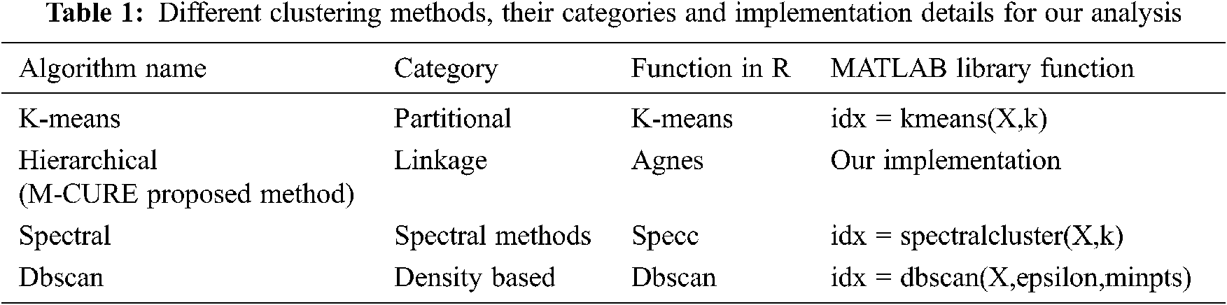
In Tab. 1, X corresponds to the data set, k is the number of clusters, epsilon refers to neighbourhood search radius and minpts is the minimum number of neighbours to identify a core point. The a priori setting of the total number of clusters is the foremost challenge with k-means algorithm. This pushes the need for other clustering algorithms based on hierarchy, representatives etc. CURE is one such effectual clustering algorithm for large databases. We have proposed a modified CURE method in this research work and the implementation is done using the R language. The experimentation contains 5 steps namely the:

a)   Installation of required packages

b)   Data Preparation

c)   Determine the relative measures

d)   Clustering analysis

e)   Clustering validation through internal and external methods

Four different data sets were used to compare our proposed technique with other state-of-the-art clustering algorithms and the quantitative measures of the cluster quality were found to be positively related with outward standards of cluster quality. The data sets include:

a)   The Barrett’s esophagus data set

b)   The rat CNS data set

c)   The yeast cell cycle data set

d)   The ovary data set

Figure 8: Snapshot of the Barrett’s esophagus data set

Fig. 8 shows the Barrett’s esophagus dataset which refers to gastroesophageal reflux disease. Patients with symptoms of indigestion and heart burn should seek medical attention before cancer development. For studying this human neoplasia, the endoscopic biopsies can be acquired from the patients. This data set consists of 7306 genes under 10 conditions [19]. Clusters can be formed to differentiate expression profiles of gastric, duodenal and squamous epithelium. The clustering algorithm performance comparison in terms of time with different methods is plotted in Fig. 9 and the readings are shown in Tab. 2.

Figure 9: Time complexity comparison of the Barrett esophagus dataset

The Rat CNS data set is obtained to examine the expression levels by reverse transcription-coupled PCR method on a set of 112 genes during rat CNS growth over 9 time points [20]. Global gene profiles were obtained from six dissimilar brain regions and three non-CNS tissues in three individual rats. It is found that the patterns were highly preserved among individual rats at the end of the study.

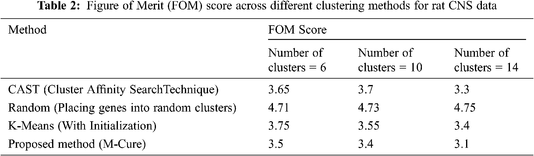
A metric called as figure of merit (FOM) is used to estimate the predictive power of the different clustering methods. FOM is defined as the is the root mean square deviation in the left-out condition of the individual gene expression levels relative to their cluster means. A small figure of merit value indicates that the clustering algorithm having high predictive power and vice versa. The FOM score comparison across different clustering methods for the RAT CNS data is shown in Fig. 10.

Figure 10: Clustering algorithm output on the rat CNS dataset

Tab. 2 shows the FOM score across different clustering methods. In the yeast data set, the promoter is the important tool for gene expression controlling. Most promoters respond to environmental signals as they are endogenous and the signals are given through up or down regulation. They change over time based on the cultivation conditions present in the industrial process.

Ovarian cancer stands as one of the leading cancer based deaths cause and the ‘curated Ovarian Data’ database is created to provide the high quality data reserve for any cancer. This gene expression medical data is obtained from 2970 cancer patients crossing 11 gene expression data from 23 studies in the form of documented expression set objects. A plot of this dataset is shown in Fig. 11.

Figure 11: Visualization of latent subclasses in the ovarian cancer dataset

The Jaccard similarity index (JC) compares members for two data sets to see which members of the set are shared and which are distinct. It's a similarity measure for the given two sets of data that ranges between 0% and 100%. The higher the percentage means that two populations are more similar. Fig. 12. represents JC for Yeast cell-cycle data set.

Figure 12: Clustering algorithm comparison on the Yeast cell-cycle data set

We have used MATLAB for exploring the microarray gene expression data. The MAT file ‘cns expression data’ contains the data matrix objects which are associated with the values and pre-processed using the RMA.

7  Conclusion

This paper presents a modified CURE algorithm for clustering the gene expression data. Though CURE can handle large databases and detect proper cluster shape with the help of representatives, they ignore the aggregate object inter-connectivity information which is addressed in this M-CURE work with the help of dynamic thresholding and effective selection of samples for clustering. The vagueness, noise and imprecision present in the gene expression data is handled effectively with the proposed algorithm and the experimental results also confirm the same. The proposed method can be extended or applied for medical sector applications for identifying and analysing severe ailments like cancer, tuberculosis etc. The complexity of biological networks along with the large number of genes increases the challenges of understanding and inferring the mass data and so the reliability of the clustering results can be improved further with the help of domain specific inputs which would be the future directions of this research work. In future, this research can be validated with machine learning and AI techniques for good clustering approach. The clustering gene expression is challenging problem, hence intelligent algorithms can process efficiently and in future it will be used and tested.

Funding Statement: The authors received no specific funding for this study.

Conflicts of Interest: The authors declare that they have no conflicts of interest to report regarding the present study.

This work is licensed under a Creative Commons Attribution 4.0 International License, which permits unrestricted use, distribution, and reproduction in any medium, provided the original work is properly cited.