DOI:10.32604/csse.2022.021750
| Computer Systems Science & Engineering DOI:10.32604/csse.2022.021750 | |
| Article |
Defect Prediction Using Akaike and Bayesian Information Criterion
1Department of Information Technology, College of Computer, Qassim University, Buraydah, Saudi Arabia
2Department of Electrical and Computer Engineering, Air University, Islamabad, Pakistan
*Corresponding Author: Saleh Albahli. Email: salbahli@qu.edu.sa
Received: 13 July 2021; Accepted: 18 August 2021
Abstract: Data available in software engineering for many applications contains variability and it is not possible to say which variable helps in the process of the prediction. Most of the work present in software defect prediction is focused on the selection of best prediction techniques. For this purpose, deep learning and ensemble models have shown promising results. In contrast, there are very few researches that deals with cleaning the training data and selection of best parameter values from the data. Sometimes data available for training the models have high variability and this variability may cause a decrease in model accuracy. To deal with this problem we used the Akaike information criterion (AIC) and the Bayesian information criterion (BIC) for selection of the best variables to train the model. A simple ANN model with one input, one output and two hidden layers was used for the training instead of a very deep and complex model. AIC and BIC values are calculated and combination for minimum AIC and BIC values to be selected for the best model. At first, variables were narrowed down to a smaller number using correlation values. Then subsets for all the possible variable combinations were formed. In the end, an artificial neural network (ANN) model was trained for each subset and the best model was selected on the basis of the smallest AIC and BIC value. It was found that combination of only two variables’ ns and entropy are best for software defect prediction as it gives minimum AIC and BIC values. While, nm and npt is the worst combination and gives maximum AIC and BIC values.
Keywords: Software defect prediction; machine learning; AIC; BIC; model selection; cross-project defect prediction
Software defect prediction is a crucial task that has been given a lot of importance recently. Researchers focus on defect prediction in order to improve the user experience and overall quality of software. When a product is introduced into the market it takes a lot of time to reach its maturity level. It passes through changes; some changes improve the product and some of them conflict with the product and cause a defect. These changes are called “defect-inducing-change” and needed to be found and removed [1]. Defect prediction is the process of predicting if the newly installed change is defect-inducing or not. There are two types of defect prediction used:
• With-in-project defect prediction
• Cross-project defect prediction
The effectiveness of a machine learning or deep learning model depends greatly on the technique used and also the quality of data used for training [2]. Usually, defect prediction models are investigated in the literature using with-in project concept that assumes the existence of previous defect data for a given project [3]. This approach is called With-in-project defect prediction. However, in practice, not all companies maintain a clear historical defect data records or sufficient data from previous versions of the project [4]. Cases like this call for an alternative approach that assembles a training set composed of known external projects. This approach is called Cross-project defect prediction and it has in recent years attracted the interest of researches due to its border applicability [5].
Machine learning and deep learning have proved to be a great source of detecting these changes on the basis of certain parameters. Machine learning and deep learning has been used for classification purposes for a long time now and has shown their worth. These techniques are supervised and need some input data. In supervised machine learning, the algorithm tries to find a pattern in the input data, and on the basis of that pattern, it tries to classify future data into a specific number of classes. Deep learning has shown better performance over the classical machine learning algorithms in many applications. Although ensemble machine learning algorithms compete with deep learning algorithms.
With-in-project defect prediction is the process in which data to train the machine learning or deep learning model is taken from the same project on which the model will be implemented for future prediction. While the cross-project defect prediction model is trained from data of one software project and is used to make predictions on data of some other software project. Cross-project defect prediction is mostly applied to the projects which are new and does not have enough data to train a machine learning or deep learning model.
Data available in software engineering for many applications is contained variability and it is not possible to say that which variable is helping in the process of prediction. In order to deal with this problem combination of different independent variables needed to be checked to find a combination that is most efficient in the prediction process. Akaike information criterion (AIC) and Bayesian information criterion (BIC) are the techniques that are used to help with this type of model selection. Model is trained for a specific combination of independent variables, AIC and BIC values are calculated and combination for minimum AIC and BIC values is selected to be the best model.
This paper deals with the problem of training a model for data of variability for both with-in-project and cross-project defect prediction. Data is first narrowed down to four variables on the basis of correlation with the output variable. Then, all the possible combinations of independent variables are used to train the Artificial Neural Network (ANN) model. In the end, AIC and BIC values for each combination are used to select the best combination. Aims of this paper are:
a) Correlation analysis of independent variables in software defect prediction dataset of six open source projects for variability analysis.
b) With-in-project and cross-project model selection on the basis of AIC and BIC
Rest of the paper is divided as follow: Section 2 highlight the previous work in the field of defect prediction and motivation for the use of AIC and BIC. Section 3 explains all the datasets used in the project along with all the variables present in those datasets. Section 4 explains the methodology used. Preprocessing of data, ANN architecture and model selection are part of this section. In short, this section explains the experimental environment. Section 5 presents all the results and gives an analysis of which model is the best and why. In the end, Section 6 concludes the paper.
2.1 Just-in-Time Software Defect Prediction
Just-in-time defect prediction is the process of finding errors inducing changes with minimum cost and there has been a lot of work done in the field using machine learning and deep learning techniques. Fan et al. [6] considered the impact of mislabeled changes on defect prediction models and took variants of SZZ i.e., B-SZZ (Basic SZZ), AG-SZZ (Annotation Graph SZZ), MA-SZZ (Meta-change Aware SZZ) and RA-SZZ (Refactoring Aware SZZ) for testing the impact. They took a prediction model trained on data labeled using RA-SZZ as a base model and tested the accuracy of other models based on it. They found that the model trained on data labeled by B-SZZ and MA-SZZ does not cause a considerable reduction in accuracy but AG-SZZ causes a considerable decline in the accuracy. Tu et al. [7] worked on better data labeling using a proposed approach known as EMBLEM. In this approach first AI labels the data and then human experts check the labels which in turn updates the AI. According to their study EMBLEM improved Popt20 and G-scores performance. Yuan et al. [8] worked on data labeling in cross-project defect prediction. The proposed method is called ALTRA which uses active learning and TrAdaBoost (Transfer learning Adaboost). They first selected similar labeled modules in the source project after analyzing the target project. Then they ask experts to label the unlabeled modules. After that TrAdaBoost was used to assign weights to labeled modules in source and target project. In the end, the model was constructed through a weighted support vector machine.
Yang et al. [9] conducted a comparative study between local and global training of models for defect prediction. For local training data was divided homogeneously using k-medoids. Logistic regression and effort-aware linear regression (EALR) was used as classification models. They found that local models work better than global models. Yang et al. [10] found that using MULTI (Multi-objective optimization) for software defect prediction sometimes results in poor performance. In order to improve the performance, they proposed three strategies: Benefit priority (BP), cost priority (CP) and combination of the two (CCB). They found that the BP-based solution improves the performance of MULTI in defect prediction. Ni et al. [11] carried out a comparative study between supervised and unsupervised defect prediction in effort aware and non-effort aware performance measures. They found that supervised models are more promising than unsupervised methods.
Tabassum et al. [12] worked on finding that to what extent cross-project data is useful. Is it useful for just starting phase of the new project or it can also work when the project is old? Chen et al. [13] carried out a comparative study between eight supervised and four unsupervised defect prediction models. The main idea was to check if different models predict the same defective modules. Xu et al. [14] considered the possibility of heterogeneous features in cross-project data and proposed a method called Multiple View Spectral Embedding (MVSE). They saw data in two different views and mapped it on a consistent space with maximum similarity.
When it comes to the use of deep learning, ANN has been used for defect prediction in different manners. Qiao et al. [15] used deep learning for defect prediction after normalizing and log-transforming the data. They found that deep learning approaches can compete with state-of-the-art approaches. Qiao et al. [16] considered selecting useful features from the overall features in order to increase the accuracy of the models.
AIC and BIC are the techniques that are used for selecting the best features from the data for training. Burnham et al. [17] give an explanation of AIC and BIC in model selection. Kuha [18] carried out a comparative study between AIC and BIC. Rodriguez et al. [19] worked on selecting different techniques for defect prediction on the basis of AIC as a selection criterion. Bettenburg et al. [20] worked on a study based on defect prediction and development effort. They trained one model globally and some local models on clustered data locally. They also used AIC and BIC as a model selection criterion.
Data from six different open-source projects was used for the study [21], which are:
• Bugzilla (4620 entries)
• Columba (4455 entries)
• JDT (35386 entries)
• Mozilla (98275 entries)
• Platform (64250 entries)
• PostgreSQL (20431 entries)
Each file consists of 14 independent variables and 1 dependent binary variable. These 14 independent variables are [22]:
• NS: Number of modified subsystems
• ND: Number of modified directories
• NF: Number of modified files
• Entropy: Distribution of the modified code across each file
• LA: Lines of code added.
• LD: Lines of code deleted.
• LT: Lines of code in a file before the current change.
• FIX: Whether or not the change is a defect fix.
• NDEV: Number of developers that changed the modified files.
• AGE: The average time interval between the last and the current change.
• NUC: The number of unique changes to the modified files.
• EXP: The developer experience in terms of the number of changes.
• REXP: Recent developer experience.
• SEXP: Developer experience on a subsystem.
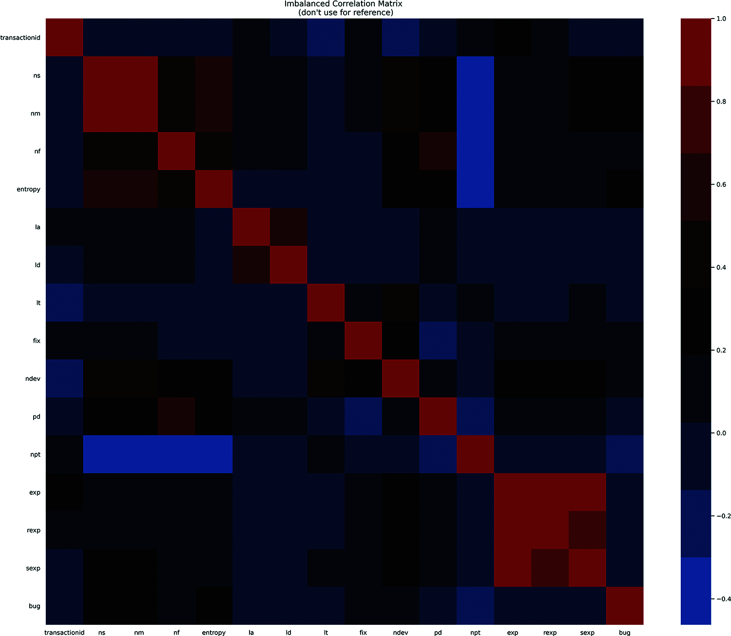
Figure 1: Heatmap of correlation matrix for Bugzilla
Tab. 1 shows all the statistics of the projects under study.
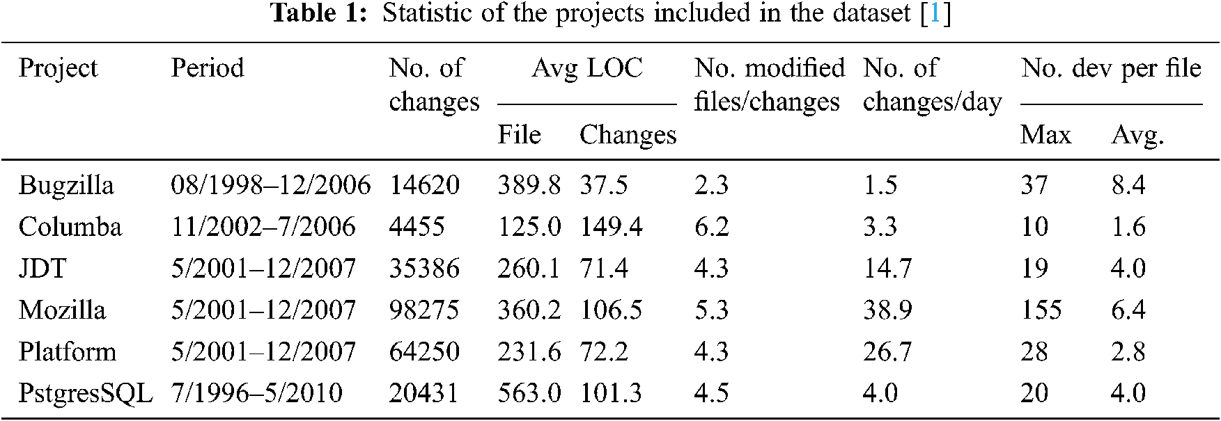
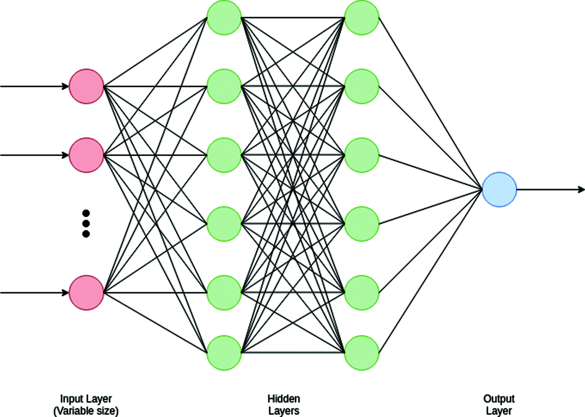
Figure 2: Architectural diagram of ANN
The overall methodology used for cross-project defect prediction models is based on the fact that not all the individual variables can’t help in better defect prediction in cross-project defect prediction. In some cases, this case is true but the fact of some variables being unnecessary can’t be ignored. Keeping this in mind, this paper proposes the use of model selection using AIC and BIC in both with-in-project and cross-project defect prediction. “Bugzilla” project was used for training the model and model selection was also applied on its basis.
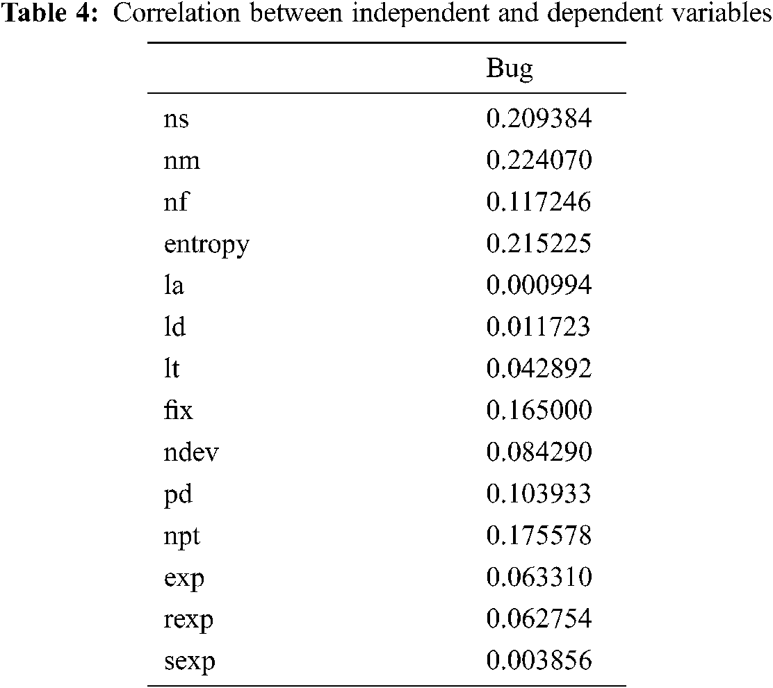
AIC and BIC are the techniques that apply model selection on all the possible pairs of variables which can be calculated by the formula of 2n where n is the total number of variables. In our case, n is 14, which makes the number of combinations to be checked equals to 214 = 16,384. It is highly inefficient to check all these combinations. To eliminate redundant variables in the first step, the correlation was used. The correlation matrix is shown in Fig. 1. The correlation value of each independent variable was observed with the dependent variable and after taking absolute of the values, top 4 valued variables were selected (ns, nm, entropy, npt). With only 4 variables left, model selection becomes fast as now there are only 16 combinations to be tested.
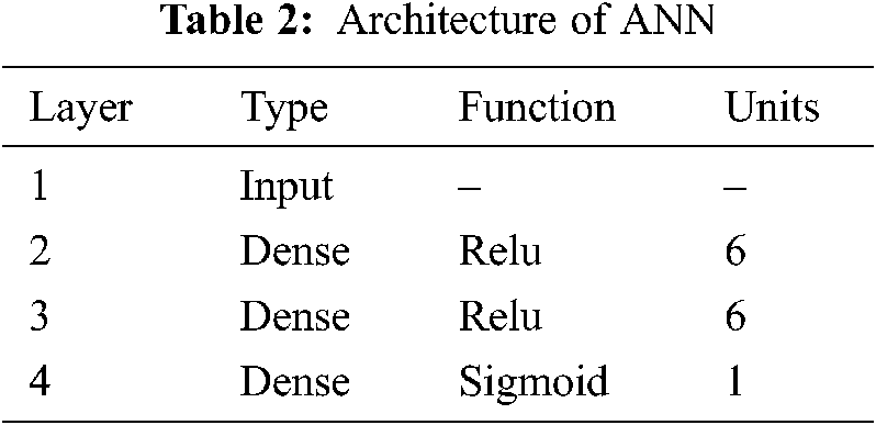
An Artificial Neural Network (ANN) was selected for binary classification of the defect prediction. ANNs are used for modelling problems and to predict the output values for given input parameter from their training values [23,24]. ANNs are a type of computer program that can be ‘taught’ to emulate relationships in sets of data. Once the ANN has been ‘trained’, it can be used to predict the outcome of another new set of input data [25]. Our ANN is designed with 1 input layer (where initial data is inserted into the neural network), 2 hidden layers (an intermediate between the input and output layers where all computation is done) and 1 output layer (which produces the final results for given inputs). The architecture of the ANN is shown in Tab. 2 and Fig. 2.
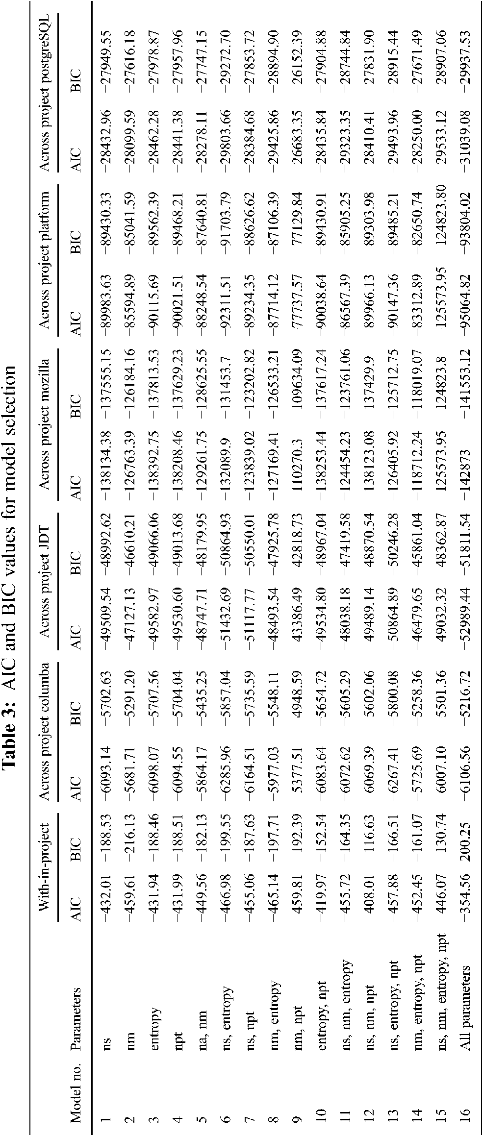
In total 16 combinations were taken ranging from single variables to all 4 variables and for reference all the 14 variables. Combinations used are shown in Tab. 3 of the results.
ANN model was trained for all the proposed combination and test accuracies were observed along with AIC and BIC values. AIC and BIC were calculated by:
Here, n is the total number of observed entries, k is the number of parameters which is equal to parameters of ANN and SSD is y–ŷ. Here y represents real outcomes and ŷ represents predicted outcomes. While calculating accuracy ŷ is rounded off to 0 or 1 but in the case of AIC and BIC while calculating SSD ŷ is not rounded off. Thus, AIC and BIC give a more accurate view of prediction i.e., how close are the values to the threshold.
At first, as described above correlation was found between all the independent variables and dependent variables meaning for the most part, there is a relation between the independent and dependent variables. Correlation values after taking absolute are shown in Tab. 4. It can be seen from Tab. 4 that ns, nm, entropy and npt are the variables with maximum correlation with output variable, bug.
After specifying 4 variables to be used for model selection are confirmed, the model was trained for all possible combinations. For with-in-project defect prediction data was divided into 80% and 20% for the train and test dataset respectively. After the model was trained it was tested for data of all the other projects in order to check cross-project defect prediction.
Tab. 3 shows the AIC and BIC values for all the possible combinations in cases of with-in-project and cross-project defect prediction. It is difficult to differentiate and compare which model has a minimum value of AIC and BIC for which model. In order to simplify it, AIC and BIC values were normalized and mapped between 0 and 1. After that average of these values was taken for selection of the optimal model. Fig. 3 shows the AIC, BIC and test accuracy plots after normalizing, and before and after averaging.
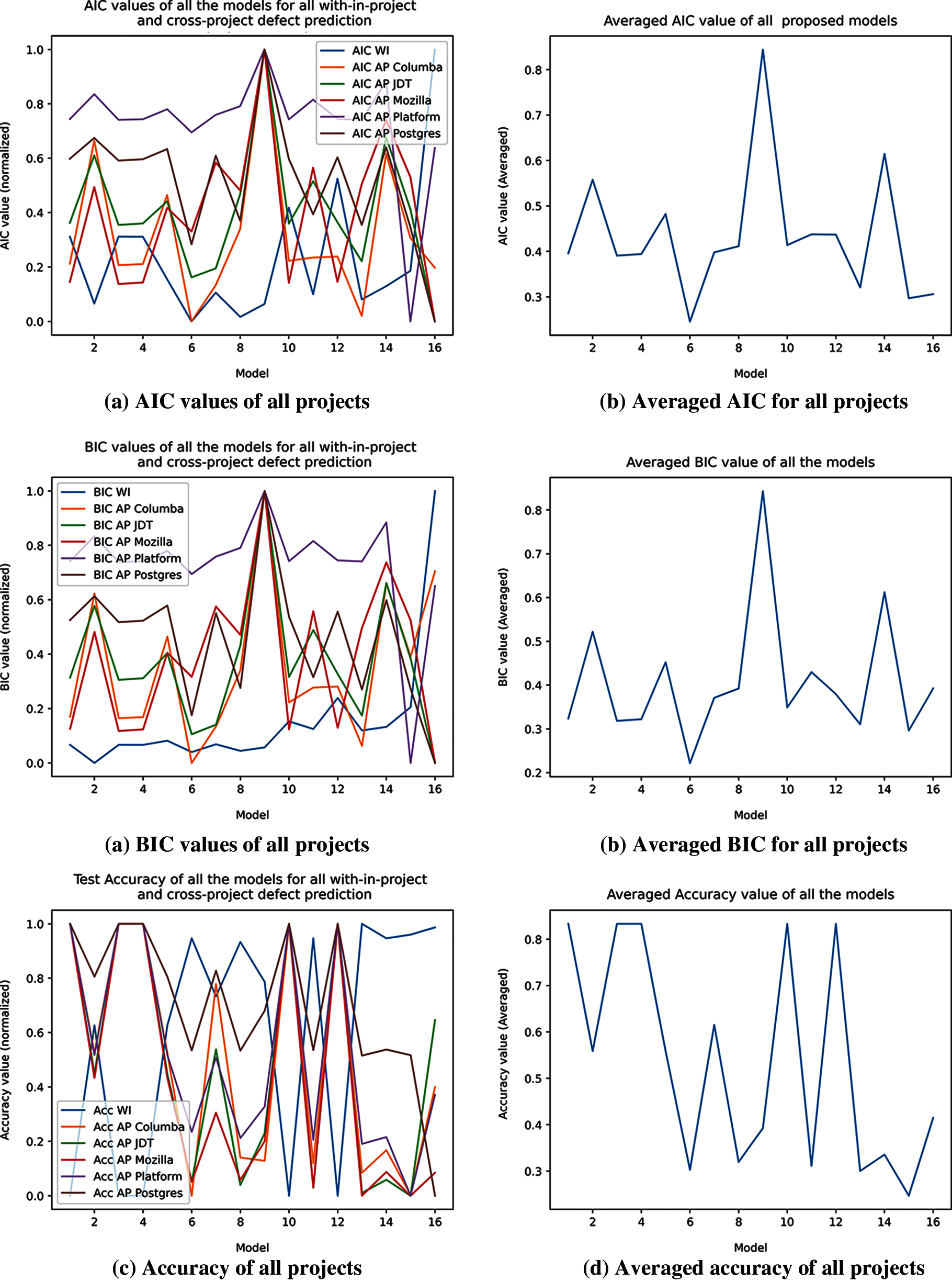
Figure 3: AIC, BIC and accuracy of all project over each model (a) AIC values of all projects (b) Averaged AIC for all projects (c) BIC values of all projects (d) Averaged BIC for all projects (e) Accuracy of all projects (f) Averaged accuracy of all projects
It is clear from the graphs that minimum values of AIC and BIC occur at model number 6, which is a combination of ns and entropy. Maximum AIC and BIC values occur at model 9 which is a combination of nm and npt. When looking at test accuracies, it can be seen that most of the models give a similar average accuracy. This is because of the fact that the model was overfitting and was predicting all the values as 0 (bug free), which is not true. Consequently, these values are ignored.
The values of the test accuracies are close and similar due to the correlation that most of them have and led to overfitting, in the future when more data has been gathered, the same experiment could still yield much better results since the model will have more dataset to train on.
Software defect prediction has been an important task in order to detect and deal with defects causing changes. It might show good performance for with-in-project defect prediction but there is no guarantee that the same case remains for cross-project defect prediction. Plus, it is not possible for each variable in assisting the prediction process and some variables might deteriorate the accuracy of prediction. Keeping this fact in mind an experiment was conducted where AIC and BIC model selection techniques were applied for highlighting the variables that are most important in the prediction process. These techniques showed that a combination of two variables “ns” and “entropy” in model training are the best fit with the minimum AIC and BIC values. Our model also showed that model 6 (ns, entropy) is the best for both with-in and cross-project defect prediction.
Acknowledgement: We would like to thank the Deanship of Scientific Research, Qassim University for covering the publication of this project.
Funding Statement: The authors received no specific funding for this study.
Conflicts of Interest: The authors declare that they have no conflicts of interest to report regarding the present study.
1. S. Albahli, “A deep ensemble learning method for effort-aware just-in-time defect prediction,” Future Internet, vol. 11, no. 12, pp. 246, 2019. [Google Scholar]
2. S. Albahli, M. Nawaz, A. Javed and A. Irtaza, “An improved faster-RCNN model for handwritten character recognition,” Arabian Journal for Science and Engineering, vol. 30, no. 1, pp. 1–5, 2021. [Google Scholar]
3. S. Herbold, A. Trautsch and J. Grabowski, “Global vs. local models for cross-project defect prediction,” Empirical Software Engineering, vol. 22, no. 3, pp. 1–37, 2017. [Google Scholar]
4. B. A. Kitchenham, E. Mendes and G. H. Travassos, “Cross versus within-company cost estimation studies: A systematic review,” IEEE Transactions on Software Engineering, vol. 33, no. 5, pp. 316–329, 2007. [Google Scholar]
5. D. Gunarathna, B. Turhan and S. Hosseini, “A systematic literature review on cross-project defect prediction,” Master’s thesis. University of Oulu, Finland, 2016. [Google Scholar]
6. Y. Fan, X. Xia, D. A. da Costa, D. Lo, A. E. Hassan et al., “The impact of changes mislabeled by SZZ on just-in-time defect prediction,” IEEE Transactions on Software Engineering, vol. 15, no. 1, pp. 1–26, 2019. [Google Scholar]
7. H. Tu, Z. Yu and T. Menzies, “Better data labelling with emblem (and how that impacts defect prediction),” IEEE Transactions on Software Engineering, vol. 56, no. 1, pp. 99, 2020. [Google Scholar]
8. Z. Yuan, X. Chen, Z. Cui and Y. Mu, “Altra: Cross-project software defect prediction via active learning and tradaboost,” IEEE Access, vol. 8, pp. 37–49, 2020. [Google Scholar]
9. X. Yang, H. Yu, G. Fan, K. Shi and L. Chen, “Local vs. global models for just-in-time software defect prediction,” Scientific Programming, vol. 2019, no. 1, pp. 1–13, 2019. [Google Scholar]
10. X. Yang, H. Yu, G. Fan, K. Yang and K. Shi, “An empirical study on progressive sampling for just-in-time software defect prediction,” in QuASoQ@ APSEC, 7th Int. Workshop on Quantitative Approaches to Software Quality, Putrajaya, Malaysia, pp. 12–18, 2019. [Google Scholar]
11. C. Ni, X. Xia, D. Lo, X. Chen and Q. Gu, “Revisiting supervised and unsupervised methods for effort-aware cross-project defect prediction,” IEEE Transactions on Software Engineering, vol. 14, no. 2, pp. 1–12, 2020. [Google Scholar]
12. S. Tabassum, L. L. Minku, D. Feng, G. G. Cabral and L. Song, “An investigation of cross-project learning in online just-in-time software defect prediction,” in Proc. of the ACM/IEEE, 42nd Int. Conf. on Software Engineering, OHIO, USA, pp. 554–565, 2020. [Google Scholar]
13. X. Chen, Y. Mu, Y. Qu, C. Ni, M. Liu et al., “Do different cross-project defect prediction methods identify the same defective mod-ules?,” Journal of Software: Evolution and Process, vol. 32, no. 5, pp. 22–34, 2020. [Google Scholar]
14. Z. Xu, S. Ye, T. Zhang, Z. Xia, S. Pang et al., “Mvse: Effort-aware heterogeneous defect prediction via multiple-view spectral embedding,” in IEEE, 19th Int. Conf. on Software Quality, Reliability and Security (QRSUSA, IEEE, pp. 10–17, 2019. [Google Scholar]
15. L. Qiao, X. Li, Q. Umer and P. Guo, “Deep learning-based software defect prediction,” Neurocomputing, vol. 385, no. 3, pp. 100–110, 2020. [Google Scholar]
16. L. Qiao and Y. Wang, “Effort-aware and just-in-time defect prediction with neural network,” PLOS ONE, vol. 14, no. 2, pp. 45–59, 2019. [Google Scholar]
17. K. P. Burnham and D. R. Anderson, “Multimodal inference: Understand ingaic and bic in model selection,” Sociological methods & research, vol. 33, no. 2, pp. 261–304, 2004. [Google Scholar]
18. J. Kuha, “Aic and bic: Comparisons of assumptions and performance,” Sociological Methods & Research, vol. 33, no. 2, pp. 188–229, 2004. [Google Scholar]
19. D. Rodriguez, J. Dolado, J. Tuya and D. Pfahl, “Software defect prediction with zero-inflated poisson models,” in MADSESE, 5th Madrilenian Seminar on Software Research. Madrid, Spain: Universidad Rey Juan Carlos, 2019. [Google Scholar]
20. N. Bettenburg, M. Nagappan and A. E. Hassan, “Think locally, act globally: Improving defect and effort prediction models,” in MSR, 9th IEEE working Conf. on Mining Software Repositories (MSRUSA, IEEE, pp. 60–69, 2012. [Google Scholar]
21. W. Fu and T. Menzies, “Revisiting unsupervised learning for defect prediction,” in Proc. of the 2017 11th Joint Meeting on Foundations of Software Engineering, pp. 72–83, 2017. [Google Scholar]
22. Y. Yang, Y. Zhou, J. Liu, Y. Zhao, H. Lu et al., “Effort-aware just-in-time defect prediction: simple unsupervised models could be better than supervised models,” in Proc of the 2016 24th ACM SIGSOFT international symposium on foundations of software engineering, New York, NY, USA, pp. 157–168, 2019. [Google Scholar]
23. A. K. Choudhury, Principles of colour and appearance measurement: Object appearance. In: The Colour Perception and Instrumental Measurement, 1st ed., vol. 1. USA: Elsevier, 2014. [Google Scholar]
24. S. Albahli, “A deep neural network to distinguish covid-19 from other chest diseases using x-ray images,” Current Medical Imaging, vol. 17, no. 1, pp. 19–29, 2021. [Google Scholar]
25. J. Lee and D. P. Almond, “A neural-network approach to fatigue-life prediction,” Fatigue in Composites, vol. 22, no. 4, pp. 569–589, 2003. [Google Scholar]
 | This work is licensed under a Creative Commons Attribution 4.0 International License, which permits unrestricted use, distribution, and reproduction in any medium, provided the original work is properly cited. |