DOI:10.32604/csse.2022.021412
| Computer Systems Science & Engineering DOI:10.32604/csse.2022.021412 | |
| Article |
Development of Efficient Classification Systems for the Diagnosis of Melanoma
1Department of Computer Science and Engineering, Shri Andal Alagar College of Engineering, Chengalpet, 603111, Tamil Nadu, India
2Department of Electronics and Communication Engineering, Kongu Engineering College, Perundurai, 638060, Erode, Tamil Nadu, India
*Corresponding Author: S. Palpandi. Email: s.palpandiphd1@gmail.com
Received: 02 July 2021; Accepted: 10 August 2021
Abstract: Skin cancer is usually classified as melanoma and non-melanoma. Melanoma now represents 75% of humans passing away worldwide and is one of the most brutal types of cancer. Previously, studies were not mainly focused on feature extraction of Melanoma, which caused the classification accuracy. However, in this work, Histograms of orientation gradients and local binary patterns feature extraction procedures are used to extract the important features such as asymmetry, symmetry, boundary irregularity, color, diameter, etc., and are removed from both melanoma and non-melanoma images. This proposed Efficient Classification Systems for the Diagnosis of Melanoma (ECSDM) framework consists of different schemes such as preprocessing, segmentation, feature extraction, and classification. We used Machine Learning (ML) and Deep Learning (DL) classifiers in the classification framework. The ML classifier is Naïve Bayes (NB) and Support Vector Machines (SVM). And also, DL classification framework of the Convolution Neural Network (CNN) is used to classify the melanoma and benign images. The results show that the Neural Network (NNET) classifier’ achieves 97.17% of accuracy when contrasting with ML classifiers.
Keywords: Melanoma; benign; classification systems; performance parameters
Melanoma is a typical type of cancer that occurs on the skin. It starts with pigment melanin-forming cells which are responsible for melanocytes-skin shading. It can spread to different parts of the system after it enters the bloodstream, affecting certain areas of the skin (the dermis). Skin melanoma is the most widely accepted type of melanoma on the skin [1]. Melanoma was granted the 2018 Nobel Prize in Medicine for finding out how to maximize the immune system to attack cancer cells, a discovery that helped in the emergence of immunotherapy drugs. As of late, the progress of practical ML classifiers prompted the development of analytical help structures for mechanization. Similarly, different ML classifiers have developed chaos within a few specialized human physiological structures [2–4].
Faruque et al. [5] have recommended a model for predicting diabetes disease using different ML algorithms such as SVM, KNN, NB, C4.5 Selection Tree. The creators assembled other diabetics and prepared additional instructions with information. Toprak [6] designed a method in which he classified 9 features based on image segmentation using an Extreme Learning Machine in the UC Irvine ML Repository database. The developed method’s performance was compared to that of other ML methods (NB, SVM, and ANN), and it proved the best result, with a score of 98.99%.
Zarshenas et al. [7] have discussed the CNN function, which analyzes different lung-related diseases. The most commonly used imaging procedure for determining the lungs is chest eczema-related disorders, yet these techniques are inaccurate. For example, lung cancer can be reasonably expected to allow for better inference. In traditional techniques, some people with pulmonary hair loss are probably unable to find anatomical structures due to overuse, for example, ribs with too many alkaline bones. These were considered inadequate when planning the NNC.
Mall et al. [8] have used mammograms to analyze the proximity of women's breast cancer cells. In the wake of different mammograms gathered from various radiographs, radiology assessments were similarly taken and contributed to CNN's preparation. Accordingly, the results were due to high accuracy and low misclassification. An overview of the papers on DL biomedical applications is distributed [9–11]. We can discover all or features of the biomedical sub-fields, yet with various applications [12,13]. By these reviews, we found an absence of harmonization for the meanings of specific sub-fields. Recently, CNN [14] has been presented in this area, and their models have been broadly acknowledged for including extraction and prompting for improved classification [15].
In such arrangements, deep discriminant features are removed by different layers as pooling, convolution, and feed-forward layers from the images by implanting an idea of Transfer Learning using tweaking and features descriptors. Notwithstanding various utilizations of CNNs in image handling, they have particularly encouraged execution in various clinical image issues like lesion classification, malignant growth, tumor determination, brain investigation, panoptic examination, and MR image combination. In the CNN applications, the image must be first extracted into a small pixel, and afterwards, the strategies must be performed on the entire superpixels. The CNN models improve the determination framework execution [16–19].
Fig. 1 displays the ECSDM proposed system’s prediction of melanoma diseases. The experiment was conducted by using dermoscopic images. The dermoscopic Melanoma and benign images are downloaded from the Kaggle database, which is initially preprocessed by using the Bottom Hat Filter (BHF) algorithm—and then preprocessing images sent to the segmentation scheme, feature extraction, and classification process. In this work, we used two different classification frameworks, as ML and DL framework. An example of ML classifiers is NB and SVM classifiers. ML is classified as the linear and polynomial regions. Another classification framework is created using the CNN classifier. We compare the prediction accuracy of both ML and DL-based CNN algorithms.
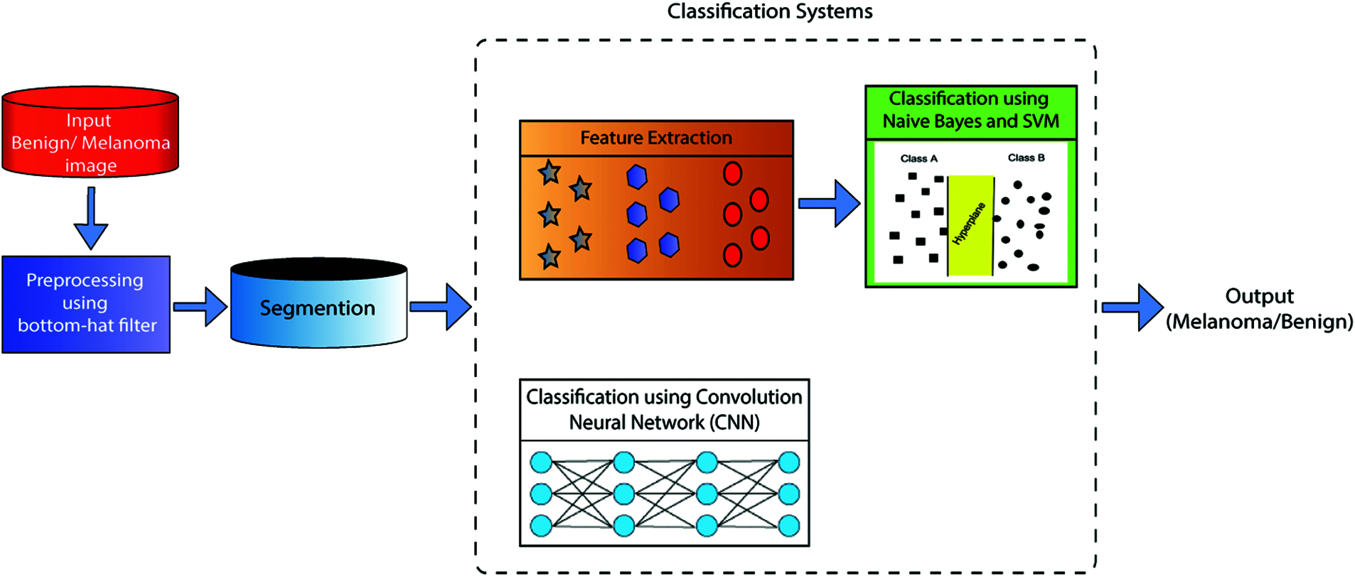
Figure 1: The proposed ECSDM
The Otsu technique is processed by converting a binary image into a binary image of any force initialized worldwide.
Initially, the melanoma and benign images are converted from colour into grayscale images and preprocess it using a BHF. To enhance the classification result. Similarly, the images that start functioning are contributed by the OTIS. The Otsu technique is processed by converting a binary image into a binary image of any force initialized worldwide.
2.1 Preprocessing – Bottom Hat Filter
A BHF improves dark spots in a white foundation. It takes away the morphological resemblance of the image from the test image. The neighbouring image performs enlargement followed by disintegration. The impact is to fill gaps and connect neighbouring objects. In numerical morphology and advanced image handling, BHF change is an activity that assists in featuring the dull spots in given images. The BHF adequately alters high-recurrence areas. BHF changes are utilized for different image handling methods, including extraction, foundation evening out, image improvement, etc. The BHF is characterized by condition, Eq. (1)
where,
2.2 Otsu Threshold-Based Image Segmentation
Otsu’s technique is a method for finding an ideal threshold dependent on the watched dissemination of pixel esteems. Otsu technique looks for the threshold that limits the intraclass fluctuation and thus expands the interclass change. This strategy depends on the pixel esteems and image space region, for example, attributes of images. Threshold-based strategy segment the image into two classes; pixel having a place with a particular scope of power esteems communicates with one class, and the remaining pixels in the image communicates with the other class. Greater separation suggests better inter-class variance between light and shadow. When the inter-class variance of the two parts varies significantly, the OTSU threshold value will be biased towards the data type with the larger variance, resulting in incorrect segmentation. When the threshold value is segmented to maximize the inter-class variance, the probability of misclassification is minimal. The following image is a two-fold image. Numerically, thresholding is characterized as beneath, Eq. (2)
where,
Empirically the chosen threshold value in our study is (normalized value).
Typically, the edges of the injuries are darkened or beaten and ragged. Also, skin lesions are not synonymous with color. Similarly, skin lesions are more significant than 6 mm.
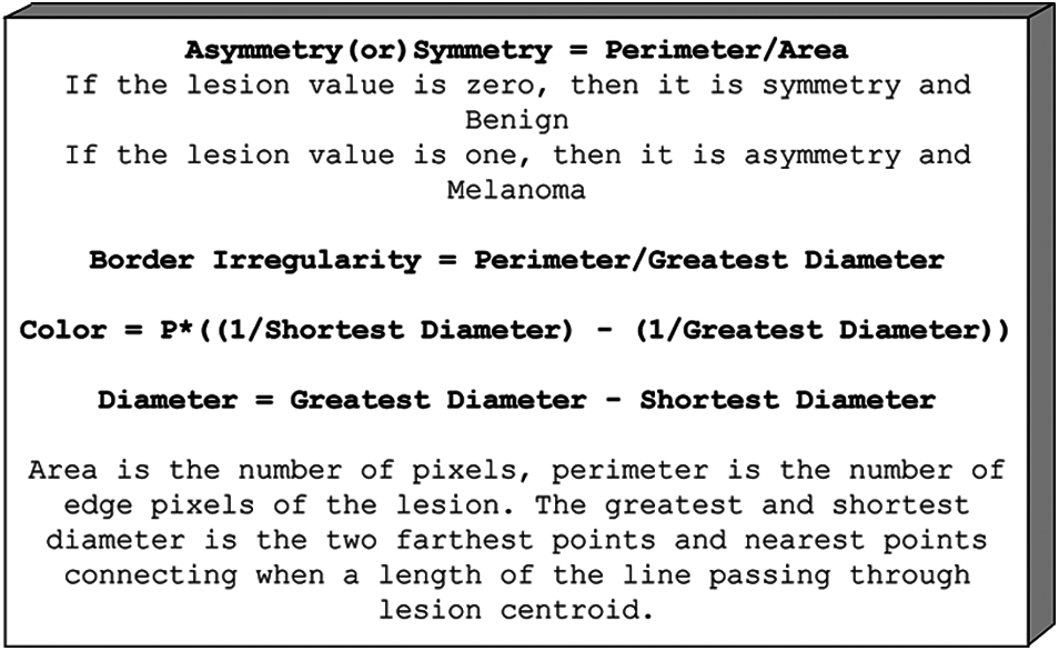
Figure 2: Melanoma feature
As a result, the characteristics of this working example include asymmetry, symmetry, border irregularity, color, diameter, LBP, and HoG, as illustrated in Fig. 2. For both melanoma and benign, preprocessed images and classification, the given frameworks have created the use of NB and SVM classifiers for the conclusion of melanoma. The above terms are all used to calculate the embraced highlights. Ojala [20] proposed the local binary pattern and were initially used for texture classification. And above all, information images are turned into grayscale. Furthermore, the local pixel, which includes the center pixel, is picked with the size of R as each pixel in the grayscale image changes. The binary example may be processed in a given image's center pixel by directly calculating the skewed pixel value and contrasting its adjacent nation pixels, as shown in Fig. 3.
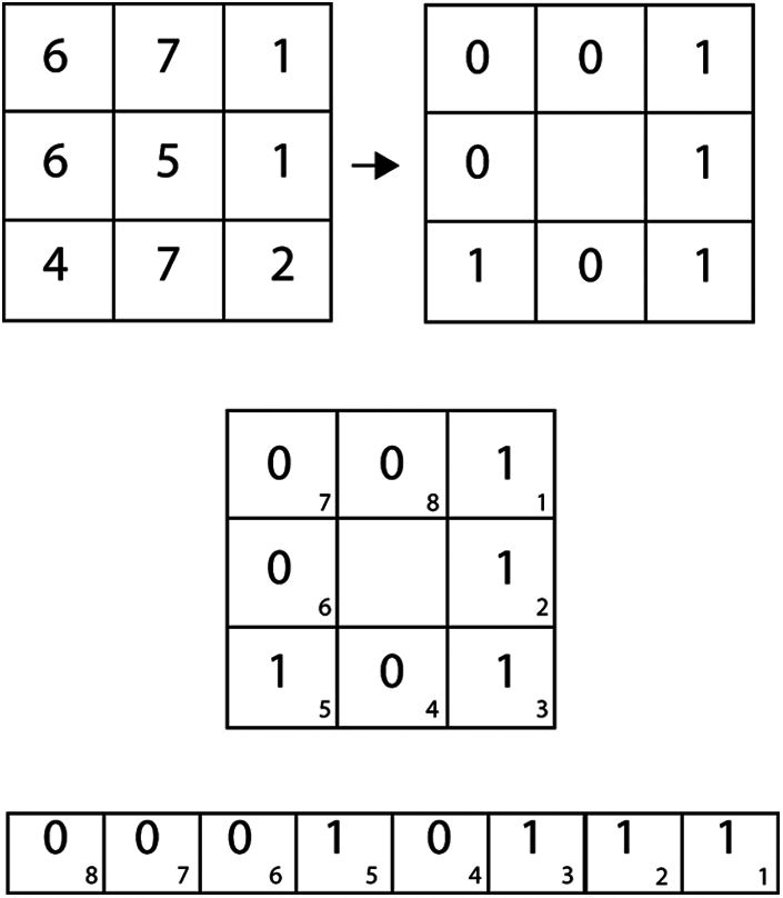
Figure 3: Local binary pattern
The estimate of the center pixel, which is more notable or equivalent than that for its neighboring country pixel at that point’s worth, will be set to 1; In either case, the value will be set to 0. After that, the LBP honor for the mid-point pixel can be determined by resizing an 8-bit binary array based on either clockwise or counter-clockwise orchestrating neighbouring pixels. For example, the registered LBP for the center pixel 4 is 23. Additionally, a HOG can be used to cut the transparent local edge directions [21].
2.4 CNN Classification Methods
The NB classifier is a Bayes theorem algorithm for object classification. NB classifiers presume that the data points are strong or Naïve independent. Spam filtering, text analysis, and medical diagnostics are significant features of NB classifiers. NB relies on the contingent possibility that a specific class has different characteristics freed from the different highlights for the class. It is sent as Eq. (3):
where
Let
The pair
From (2) and (3), it follows that Eq. (6)
Therefore
The primary way information is to be released as a place item
A kernel is used in training calculations. All direct SVM models are still carried out as a straight detachment. Since the previous approximation, as far as practical, supplanting the dot with kernel work is yet an alternative space. Using Polynomial Kernel Functions in SVM, Eq. (8)
Falling capabilities require computation. Accordingly, they are not challenging to take action. It remains to know which kernel capacity may be related to a given potential. In this manner, the customer operates from “E Trial and Error”. A favorable condition is that the main parameters are required when doing a SVM training kernel task ‘k’.
2.4.3 Convolution Neural Network
A typical CNN architecture is shown in Fig. 4. In this work, an intensive ML model is built using the CNN with LetNet design. Pooling layers include convolutional, two actuation mechanisms, and LeNet engineering, followed by a fully connected layer, initiation, another fully connected, and finally a softmax classifier. The use of the CNN classifier model is executed in Keras and Python with LeNet network design. Similarly, 5340 images are aggregated from the Kaggle database, with 90% used for training and 10% used to study the classifier’s presentation.
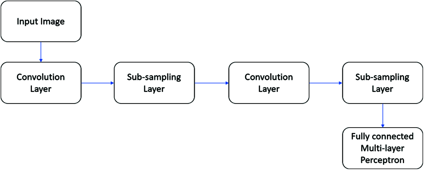
Figure 4: A typical CNN architecture
In short, the received CNN design can be [INPUT-CONV-RELU-POOL-FC], which is clarified as
• Input as (32 × 32 × 3) captures the raw pixel projections of the image. In contrast, the image of 32 widths, 32 heights, and with 3 RGB shading channels CONV layer yield data of a neuron registering a blur item between the regions associated with surrounding regions in the information, each with its load and a small area they are associated within the amount of data. This can bring about volume. For example, the (32 × 32 × 42) filter size is set to 42.
• Relu layer maximum (0, x) thresholding at zero applies an element-wise activation function. The shape of this leaf volume is unaltered (32 × 32 × 42).
• The pooling layer plays an observation activity with spatial measurements (width, height), bringing about the volume, for example, below (16 × 16 × 42).
• Between FC or fully connected layer of two classifications (benign or melanoma), the amount of size (1 × 1 × 2), where each one of the two numbers brings about a comparison of a class score, for example, class F1 Score statistics.
For example, a total of six measurements, Sensitivity, Specificity, Positive Predictive Value (PPV), Negative Predictive Value (NPV), and F1 Score, are fitted to assess the exposition of two specific classification frameworks Scores. The accompanying position is used to perform the measurement operation of both classification frameworks. Fig. 5 shows the confusion matrix formulae.
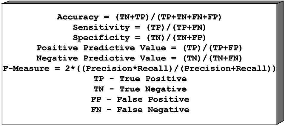
Figure 5: Confusion matrix
The typical dermoscopy melanoma, benign images, and OTIS images are shown in Figs. 6a and 6b; Figs. 7a and 7b, respectively.

Figure 6: (a) Classic dermoscopy melanoma and (b) Segmented image

Figure 7: (a) Classic dermoscopy benign and (b) Segmented image
Figs. 8a and 8b indicate a typical yield of NNETs of inflection using a classification framework. When train images and test images are given to the CNN classifier, it is observed that the CNN classifier can effectively classify tests of benign and melanoma images.

Figure 8: Result of classification system using (a) CNN Benign (b) Melanoma
Fig. 9 shows the exhibition parameters of the NB classifier using a classification framework. The NB classifier’s accuracy is 69.4%, and the performance measurement is imperfect when contrasted with different classifiers.
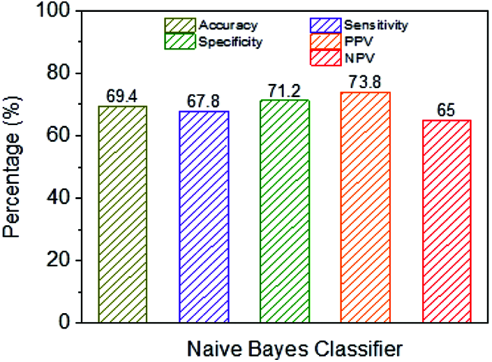
Figure 9: Performance analysis of NB classifier
Figs. 10a and 10b show the classification framework using a SVM classifier. It has been proved that the proposed SVM with polynomial kernels is dramatically different from that of SVM with linear kernels. Furthermore, the polynomial kernel SVM classifier has a better Outcome than the SVM classifier.

Figure 10: Performance metrics of Linear SVM and (b) Polynomial SVM Kernel
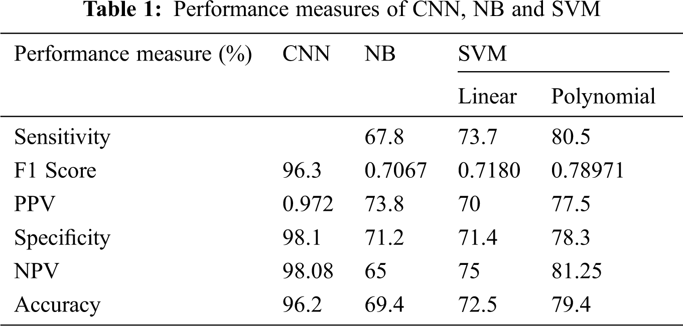
Fig. 11 shows the classification performance using CNN. The CNN classifier has an accuracy of 97.17% in addition to NB, linear and polynomial kernel SVM, which have been observed as lower performance parameters. For example, sensitivity is higher when contrasted with different classifiers. For example, Specificity, NPV, and PPV are higher when compared to SVM classifiers. From the results, it has been demonstrated that the use of the classification framework exhibits CNN classifiers acceptable when the classification framework is skewed with the presentation of NB, SVM and used with direct and polynomial kernels.
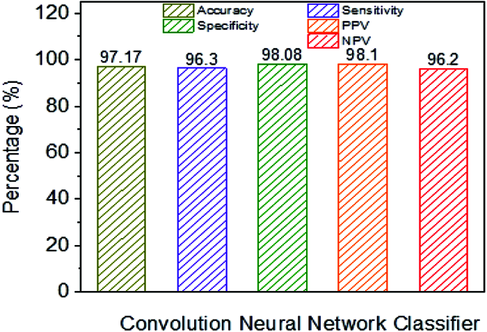
Figure 11: Performance analysis CNN classifier
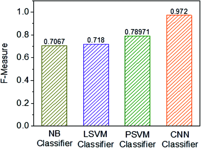
Figure 12: Performance analysis of F1 Score
Fig. 12 shows the F1 Score of four individual classifiers, for example, NB, Linear SVM, Polynomial SVM, and CNN classifier. Furthermore, it has been observed that the F1 Score of the CNN classifier is 0.972%, which is higher when contrasted with other embraced classifiers. Along these lines, the classification framework of CNN classifier use is exceptionally productive when using other classification frameworks instead of NB, LSVM, and PSVM classifiers (Tab. 1).
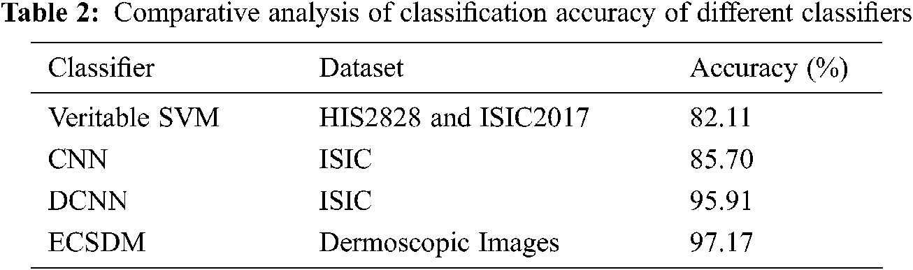
Tab. 2 shows the comparative analysis of the classification accuracy of the proposed ECSDM model with the existing CNN approach. Lingaraj et al. [22] suggested the veritable SVM to classify Melanoma to use the HIS2828 and ISIC2017 datasets and achieved the accuracy of 82.11% and 88.10% on HIS2828 and ISIC2017 medical image datasets. Li et al. [23] have used the CNN method to achieve the classification accuracy of 85.70%. Also, Hosny et al. [24] have projected the DCNN method to achieve an accuracy of 95.91%; however, our proposed ECSDM model achieves the classification accuracy of 97.17%, respectively.
In this work, classification frameworks of melanoma are investigated. The HOG and local binary patterns are used to preprocess the images. Then, the classification frameworks as ML and DL classifiers are used. Naive Bayes and SVM are the ML classifiers. In this study, the DL technique as CNN achieves a better classification performance than Naive Bayes and SVM to diagnose melanoma or benign. Results display presentation measurements, for example, accuracy, sensitivity, specificity, PPV, NPV, and rotate using a classification framework NNET classifier of F1 Score that is high (0.972) when the classification framework exhibits measurement using ML classifiers. For example, with odd direct and polynomial kernels, NB, and SVM classifiers. Additionally, it has been observed that the proposed ECSDM-CNN classifier exhibits higher (97.17%) than any classifiers already presented, which have an accuracy of 90.3%. When the network is designed, test images can be gathered by using cameras for classification frameworks, and finding melanoma should be as powerful as possible in the future.
Funding Statement: The authors received no specific funding for this study.
Conflicts of Interest: The authors declare that they have no conflicts of interest to report regarding the present study.
1. A. Dascalu and E. O. David, “Skin cancer detection by deep learning and sound analysis algorithms: A prospective clinical study of an elementary dermoscope,” EBioMedicine, vol. 43, no. 1, pp. 107–113, 2019. [Google Scholar]
2. D. Venugopal, T. Jayasankar, M. Yacin Sikkandar, M. Ibrahim Waly, V. Pustokhina et al., “A novel deep neural network for intracranial haemorrhage detection and classification,” Computers Materials & Continua, vol. 68, no. 3, pp. 2877–2893, 2021. [Google Scholar]
3. Q. Tao and R. Veldhuis, “Robust biometric score fusion by naive likelihood ratio via receiver operating characteristics,” IEEE Transactions on Information Forensics and Security, vol. 8, no. 2, pp. 305–313, 2013. [Google Scholar]
4. Q. Wu, X. Shen, Y. Li, G. Xu, W. Yan et al., “Classifying the multiplicity of the EEG source models using sphere-shaped support vector machines,” IEEE Transactions on Magnetics, vol. 41, no. 5, pp. 1912–1915, 2005. [Google Scholar]
5. M. Faruque and I. H. Sarker, “Performance analysis of machine learning techniques to predict diabetes mellitus,” in Int. Conf. on Electrical, Computer and Communication Engineering (ECCECox's Bazar, Bangladesh, pp. 1–4, 2019. [Google Scholar]
6. A. Toprak, “Extreme Learning Machine (ELM)-based classification of benign and malignant cells in breast cancer, Medical Science Monitor,” International Medical Journal of Experimental and Clinical Research, vol. 24, no. 4, pp. 6526–6537, 2018. [Google Scholar]
7. A. Zarshenas, J. Liu, P. Forti and K. Suzuki, “Separation of bones from soft tissue in chest radiographs: Anatomy-specific orientation-frequency-specific deep neural network convolution,” Medical Physics, vol. 46, no. 5, pp. 2232–2242, 2019. [Google Scholar]
8. S. Mall, P. C. Brennan and C. Mello-Thoms, “Modeling visual search behavior of breast radiologists using a deep convolution neural network,” Journal of Medical Imaging, vol. 5, no. 3, pp. 35489–35502, 2018. [Google Scholar]
9. S. H. Kassani and P. H. Kassani, “A comparative study of deep learning architectures on melanoma detection,” Tissue and Cell, vol. 58, no. 5, pp. 76–83, 2019. [Google Scholar]
10. C. Cao, F. Liu, H. Tan, D. Song, W. Shu et al., “Deep learning and its applications in biomedicine,” Genomics, Proteomics & Bioinformatics, vol. 16, no. 1, pp. 17–32, 2018. [Google Scholar]
11. D. Ravi, C. Wong, F. Deligianni, M. Berthelot, J. Andreu Perez et al., “Deep learning for health informatics,” IEEE Journal of Biomedical and Health Informatics, vol. 21, no. 7, pp. 4–21, 2017. [Google Scholar]
12. W. Jones, K. Alasoo, D. Fishman and L. Parts, “Computational biology: Deep learning,” Emerging Topics in Life Sciences, vol. 1, no. 3, pp. 257–274, 2017. [Google Scholar]
13. S. Sudhakar, L. Arokia Jesu Prabhu, V. Ramachandran, V. Priya, R. Logesh et al., “Images super-resolution by optimal deep AlexNet architecture for medical application: A novel DOCALN,” Journal of Intelligent & Fuzzy Systems, vol. 39, no. 6, pp. 8259–8272, 2020. [Google Scholar]
14. S. Min, B. Lee and S. Yoon, “Deep learning in bioinformatics,” Briefings in Bioinformatics, vol. 18, no. 5, pp. 851–869, 2016. [Google Scholar]
15. S. B. Shrestha and Q. Song, “Adaptive learning rate of SpikeProp based on weight convergence analysis,” Neural Networks, vol. 63, no. 12, pp. 185–198, 2015. [Google Scholar]
16. Y. Li and L. Shen, “Skin lesion analysis towards melanoma detection using deep learning network,” Sensors, vol. 18, no. 2, pp. 548– 556, 2018. [Google Scholar]
17. S. Sudhakar, V. Priya, A. Syed Musthafa, R. Logesh, P. Saravanan et al., “A fuzzy-based high-resolution multi-view deep CNN for breast cancer diagnosis through SVM classifier on visual analysis,” Journal of Intelligent & Fuzzy Systems, vol. 39, no. 6, pp. 8573–8586, 2020. [Google Scholar]
18. Y. Zhou, J. Xu, Q. Liu, C. Li, Z. Liu et al., “A radiomics approach with CNN for shear-wave elastography breast tumor classification,” IEEE Transactions on Biomedical Engineering, vol. 65, no. 9, pp. 1935–1942, 2018. [Google Scholar]
19. L. Zhang, F. Yin and J. Cai, “A multi-source adaptive MR image fusion technique for MR-guided radiation herapy,” International Journal of Radiation Oncology, vol. 102, no. 3, pp. 541–552, 2018. [Google Scholar]
20. T. Ojala, M. Pietikainen and T. Maenpaa, “Multiresolution grayscale and rotation invariant texture classification with local binary patterns,” IEEE Transactions on Pattern Analysis and Machine Intelligence, vol. 24, no. 7, pp. 971–987, 2002. [Google Scholar]
21. N. Dalal and B. Triggs, “Histograms of oriented gradients for human detection,” IEEE Computer Society Conf. on Computer Vision and Pattern Recognition (CVPR'05), vol. 1, no. 13, pp. 886–893, 2005. [Google Scholar]
22. M. Lingaraj, A. Senthilkumar and J. Ramkumar, “Prediction of melanoma skin cancer using veritable support vector machine,” Annals of the Romanian Society for Cell Biology, vol. 18, no. 02, pp. 2623–2636, 2021. [Google Scholar]
23. Y. Li and L. Shen, “Skin lesion analysis towards melanoma detection using deep learning network,” Sensors, vol. 18, no. 2, pp. 556–568, 2018. [Google Scholar]
24. K. M. Hosny, M. A. Kassem and M. M. Foaud, “Classification of skin lesions using transfer learning and augmentation with Alex-net,” PLoS One, vol. 14, no. 4, pp. 55–72, 2019. [Google Scholar]
 | This work is licensed under a Creative Commons Attribution 4.0 International License, which permits unrestricted use, distribution, and reproduction in any medium, provided the original work is properly cited. |