DOI:10.32604/csse.2022.021698
| Computer Systems Science & Engineering DOI:10.32604/csse.2022.021698 | |
| Article |
Automated Deep Learning Based Cardiovascular Disease Diagnosis Using ECG Signals
1Department of Computer Science & Engineering, SNS College of Technology, Coimbatore, 641035, India
2Department of Information Technology, Karpagam Institute of Technology, Coimbatore, 641105, India
*Corresponding Author: M. Santhosh. Email: santhoshsnsphd@gmail.com
Received: 10 July 2021; Accepted: 11 August 2021
Abstract: Automated biomedical signal processing becomes an essential process to determine the indicators of diseased states. At the same time, latest developments of artificial intelligence (AI) techniques have the ability to manage and analyzing massive amounts of biomedical datasets results in clinical decisions and real time applications. They can be employed for medical imaging; however, the 1D biomedical signal recognition process is still needing to be improved. Electrocardiogram (ECG) is one of the widely used 1-dimensional biomedical signals, which is used to diagnose cardiovascular diseases. Computer assisted diagnostic models find it difficult to automatically classify the 1D ECG signals owing to time-varying dynamics and diverse profiles of ECG signals. To resolve these issues, this study designs automated deep learning based 1D biomedical ECG signal recognition for cardiovascular disease diagnosis (DLECG-CVD) model. The DLECG-CVD model involves different stages of operations such as pre-processing, feature extraction, hyperparameter tuning, and classification. At the initial stage, data pre-processing takes place to convert the ECG report to valuable data and transform it into a compatible format for further processing. In addition, deep belief network (DBN) model is applied to derive a set of feature vectors. Besides, improved swallow swarm optimization (ISSO) algorithm is used for the hyperparameter tuning of the DBN model. Lastly, extreme gradient boosting (XGBoost) classifier is employed to allocate proper class labels to the test ECG signals. In order to verify the improved diagnostic performance of the DLECG-CVD model, a set of simulations is carried out on the benchmark PTB-XL dataset. A detailed comparative study highlighted the betterment of the DLECG-CVD model interms of accuracy, sensitivity, specificity, kappa, Mathew correlation coefficient, and Hamming loss.
Keywords: Biomedical signals; 1-dimensional signal; electrocardiogram; artificial intelligence; deep learning; cardiovascular disease; decision making
Cardiovascular Disease (CVD) is the major reason for human mortality, which is accountable for thirty-one percentage of global mortalities in 2016 [1], from which eighty-five percentage occurred because of heart attack. The yearly burden of CVD on American and European economies is calculated to be $555 billion and €210 billion, correspondingly. The conventional CVD diagnosis model is depending upon single person's medicinal history and investigations. This result is interpreted based on set of quantitative medicinal variables for classifying the person according to the taxonomy of medicinal disease. Medically, cardiovascular diseases are frequently acquired using arrhythmia. Severe arrhythmia could result in heart failure/sudden death [2]. Thus, accurate and timely recognition of arrhythmia is necessary and urgent. Electrocardiogram (ECG) is a 1-dimensional physiological signal which describes the state of the heart, is very important to detect and diagnose arrhythmia.
ECG analyses were determined as the fundamental cardiovascular pathology diagnoses in the present century. The ECG signal reflects the electrical activity of the heart. Therefore, heart rhythm disorder/alteration in the ECG waveform is evidence of basic cardiovascular issues like arrhythmias. Non-invasive arrhythmia diagnoses are depending upon typical twelve leading ECGs that measure electrical potential from ten electrodes located at distinct portions of the body surface, 6 in the chest, and 4 in the limbs. To give an efficient medication for arrhythmias, an earlier diagnosis is significant. Globally millions of ECG records are gathered yearly, mostly analyzed automatically and interpreted via computers [3,4]. It executes the need for ECG interpretation approaches for accurate and fast however person and device autonomous. The extensive digitization of ECG information combined with the growth of DL techniques that could process huge number of raw data has presented novel opportunities to improve the automatic ECG interpretation. In fact, DNN has currently attained cardiologist level classification efficiency if trained on a huge (n = 91,232) dataset of raw ECG records. But, presented ECG datasets are frequently lesser that creates complexity for attaining required efficiency level.
Earlier recognition of specific kinds of transient, short-term/infrequent arrhythmias needs long-term observing (over 24 h) of electrical activity of the heart. The rapid growth of digital industry was enabled to improvement of data acquisition, devices, and CAD approaches. The open-access to ECG database has result in the improvement of several approaches and techniques for CAD ECG arrhythmia classification in past few years, raising the productive cross disciplinary effort where the physicists’ engineers, and nonlinear dynamics scientists are no strangers [5]. Nearly each CAD ECG classification method includes 4 major phases, such as FS, pre-processing of ECG signal, feature extraction, classification creation, and heartbeat recognition. Recently, they have observed significant developments in automated ECG interpretation methods. Particularly, DL based techniques have attained or exceeded cardiologist level efficiency for certain sub-tasks [6,7] or allowed statements are highly complex for making cardiologists, for instance, precisely infer age and gender from the ECG. Because of obvious easiness and decreased dimension related to imaging data, the broader ML communities have attained several attentions in ECG classification as recorded via several studies.
This study designs automated deep learning based 1D biomedical ECG signal recognition for cardiovascular disease diagnosis (DLECG-CVD) model. The DLECG-CVD model involves different stages of operations namely pre-processing, feature extraction, hyperparameter tuning, and classification. At the same time, improved swallow swarm optimization (ISSO) algorithm based deep belief network (DBN) model is applied to derive a set of feature vectors. In addition, extreme gradient boosting (XGBoost) classifier is employed to allocate proper class labels to the test ECG signals. For examining the enhanced diagnostic outcome of the DLECG-CVD model, a series of experimentations take place on the benchmark PTB-XL dataset.
The key contribution of the paper is given as follows.
▪ An efficient 1D biomedical ECG signal recognition model using DLECG-CVD model is presented for cardiovascular diseases. To the best of our knowledge, the DLECG-CVD model has been never presented in the literature.
▪ A novel ISSO based feature selection technique is introduced by incorporating the concepts of levy flight to the SSO algorithm in order to avoid the local optima problem. The design of ISSO algorithm shows the novelty of the work.
▪ Besides, the inclusion of ISSO algorithm as a hyperparameter optimizer helps to improve the classification performance of the DLECG-CVD model for unseen data.
▪ A detailed experimental validation process takes place using PTB-XL dataset and examined the outcomes under several dimensions.
The organization of the paper is given as follows. Section 2 reviews the recent state of art ECG recognition techniques. Section 3 discusses the materials and methods involved in the proposed model. Next, section 4 offers the detailed experimental analysis and section 5 draws the conclusions.
This section offers a comprehensive survey of recently developed ECG recognition and classification models. In Li et al. [8], the morphology and rhythm of heartbeats are merged to 2D data vector to process consequently using CNN which includes biased dropout and adaptive learning rate approaches. The result demonstrates the projected CNN module is efficient to detect abnormal heartbeats/arrhythmias by automated feature extraction. Weimann and Conrad [9] used DCNN for classifying raw ECG records. But, training CNN for ECG classification frequently needs a huge number of annotated instances that are costly to obtain. In this study, they address the issue with the help of TL technique. Initially, they pretrain CNN on the large public dataset of continued raw ECG signals. Then, they fine-tune the network on a smaller dataset for classification of Atrial Fibrillation that is one of the popular heart arrhythmia.
In Pandey et al. [10], an 11-layer DCNN module is presented to classification of MIT-BIH arrhythmia database into five classes based on ANSI AAMI principles. In this CNN module, they implemented a comprehensive end to end structure of the classification technique and employed with no other denoising processes of the database. The main benefit of the novel method was presented in the several classifications that would decrease and should identify, and segmented the QRS complex, avoided. This MIT-BIH database was artificially over-sampled for handling the minority class, class imbalance challenge utilizing SMOTE method. Jeon et al. [11] presented a baseline module with RNN for ECG classification. Moreover, they proposed a light weighted module with combined RNN to accelerate the predictive time on CPU.
Shaker et al. [12] presented a new data augmentation model utilizing GAN technique for restoring the balance of dataset. The 2 DL an end-to-end method and a 2-phase hierarchical approach depending upon DCNN is utilized for eliminating hand engineering features with the combination of feature reduction, classification, and feature extraction to a single learning technique. Nurmaini et al. [13], DL is presented in the fine-tuning and pre-training stages for producing an automatic feature depiction to multi class classification of arrhythmia condition. In pre-training stage, stacked DAE and AE are utilized to feature learning; in fine-tuning stage, DNN is designed as classifiers. Huang et al. [14] presented an accurate classification model based on intelligent ECG utilizing FCResNet. In this introduced system, the MOWPT gives a comprehensive time scale paving pattern and possesses time invariance features that are employed for decomposing the real ECG signal to sub signal samples of various scales. Then, the sample of five arrhythmia forms is employed as input to the FCResNet; hence, ECG arrhythmia types are categorized and recognized. Han et al. [15] enhanced a technique for constructing a smoothed adversarial instance to ECG tracing which is not visible to human expert's analysis and shows that the DL technique to detect arrhythmia from single lead ECG is vulnerable to adversarial attacks. Furthermore, they offer common method to collate and perturb known adversary instances for creating many novel ones.
Wang et al. [16] presented an automated ECG classification technique depending upon Continuous Wavelet Transform (CWT) and Convolutional Neural Network (CNN). The CWT is utilized for decomposing ECG signals to attain various time frequency modules, and CNN is utilized for extracting features in two-dimensional scalogram consist of aforementioned modules. Consider the nearby R peak interval (named RR interval) is beneficial to diagnose arrhythmia, 4 RR interval features are combined and extracted by CNN features to input for fully connected (FC) layer to ECG classification. Peimankar et al. [17] proposed a DL module for real time segmentation of heartbeats. The presented DENS ECG technique, integrates LSTM and CNN module for detecting offset, onset, and peak of distinct heartbeat waveforms like NW, T-waves, P-waves, and QRS complexes. By utilizing ECG as input, the module learns for extracting higher level feature by trained procedure that contrasting to other traditional ML based techniques, removes the feature engineering stage. In Wang et al. [18], a new CNN with NCBAM is presented for classifying automatic ECG heartbeats. Approaches: this presented technique contains 33-layer CNN framework accompanied by NCBAM module. At first, pre-processed ECG signals are provide for CNN framework for extracting the channel and spatial features. Additionally, longer range dependences of illustrative features together with channel and spatial axes are taken using non-local attention. Lastly, the temporal, spatial, and channel data of ECG is combined using learned matrix.
This study utilizes PTB-XL dataset [19] which comprises 21837 ECG signals of 10 s duration from 18885 persons in which 52% of persons are male and the remaining 48% of the persons are female. The ECG data employed for annotation follows the SCP-ECG standard and are allocated to 3 non-mutually exclusive classes such as diagnostic, form, and rhythm. Totally, 71 distinct records have existed that decomposed into 44 diagnostics, 12 rhythm, and 19 form statements. Moreover, the PTB-XL data encompasses 5 classes such as normal ECG (NORM), conduction disturbance (CD), myocardial infarction (MI), hypertrophy (HYP), and: ST/T changes (STTC). Furthermore, a total of 24 subclass labels are also provided.
3.2 Overall System Architecture
The overall system architecture of the presented model is illustrated in Fig. 1. The figure showcases that the input ECG signals are primarily pre-processed to convert into a compatible format. Then, the DBN model is applied to extract a useful set of feature vectors. At the same time, the ISSO algorithm is employed to optimize the hyperparameters of the DBN model. At last, the XGBoost classifier is used to allocate the class labels of the input ECG signals. These processes are briefly discussed in the succeeding subsections.
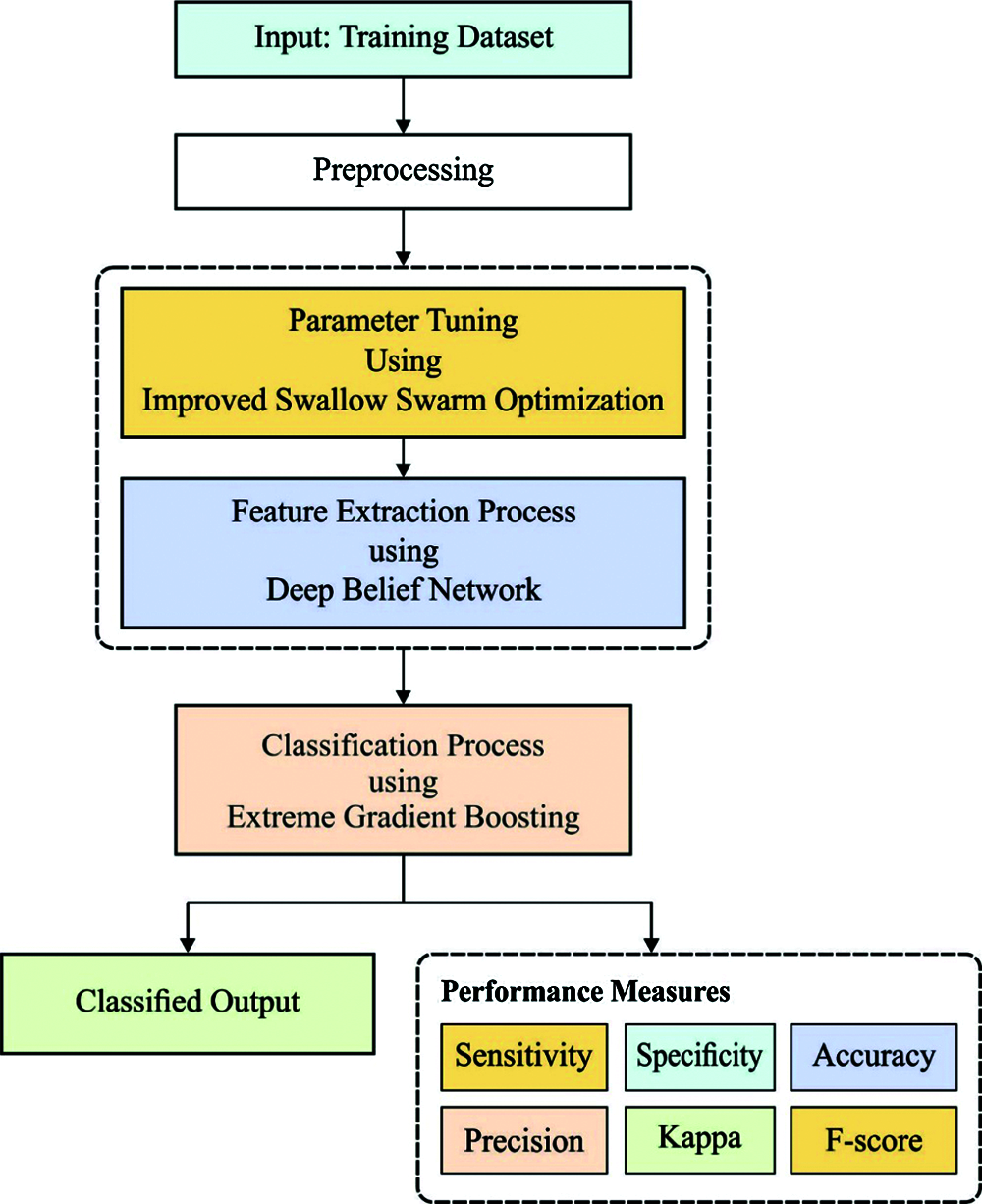
Figure 1: The working process of DLECG-CVD model
During data pre-processing, a collection of 3000 ECG signals is used for experimental analysis. As a set of 35 ECG signals include NULL as class label, they get eliminated from the dataset and the remaining 2965 ECG records are employed for simulation. In addition, a sampling rate of 100 is selected among the two sampling rates of 100 and 500 from the dataset.
Once the 1-D ECG signals are processed, they are inputted to the DBN model to filter the required feature vectors. The DBN presented by Hinton et al. [20] is a typical DNN method that has various RBMs and classifier layers. In standard DNNs, the trained DBN has unsupervised pre-trained of deep RBMs and supervised fine-tuned of the classifier layer. The DBN depicts an optimal feature extraction efficiency and most suitable to feature learning in data. The DBN is a representative FC networks which is simpler than other classic DNNs. It allows the presented model in rule extraction and insertion as to DBN for ECG signal recognition. All RBMs are combined of visible layer which includes the visible unit
where ωij refers the connection weight amongst visible units vi if whole number is I and hidden units h. When the whole number is J, bi and aj represents the bias terms of visible and hidden units correspondingly [21]. The joint distribution of the entire units is estimated dependent upon the energy function E (v, h; θ) as given in Eq. (2):
where
where δ denotes the logistic function, for instance, δ(x) = 1/1 + exp(x). The RBMs are trained for maximizing the joint probabilities. It is formed by stacking multiple RBMs, in which the output of lth layer (hidden units) is employed as input of l + 1th layer (visible units). The trained process of DBN is generalized as to 2 stages like pre-training and fine-tuning. During the pre-training stage, the data is provide for visible layers of an initial RBM and changed into hidden layers that are frequently applied from next RBM. Next, the layer-to-layer unsupervised trained is complete, and feature learnt automatic by DBN in the provided data is feed as to classifier layer of DBN. Lastly, fine-tuning is carried out on the classifier layer for enhancing DBN. Fig. 2 demonstrates the architecture of DBN model.
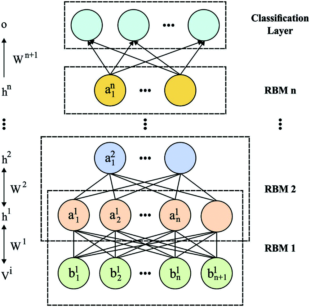
Figure 2: The structure of DBN
3.5 Design of ISSO Algorithm for Hyperparameter Optimization
For improving the performance of the DBN model, its hyperparameters are optimally tuned by the use of ISSO algorithm. SSO is a population based metaheuristic dependent technique presented by Neshat et al. [22]. Initially, in all iterations, the population is sorted depending upon the value of objective functions. Afterward, the subsequent parts are allocated as follows:
1) The head leader (HL) is the particles with an optimal value of objective functions;
2) The local leaders (LL) are l particles which follow the HL according to the value of objective functions;
3) The random particles are k particle with worse value of objective functions;
4) Explorers are every particle.
At the present iteration, HLs do not transfer, performing as beacons to explore particles that, sequentially, explores the search space among the adjacent LL and HL. The explorer particle varies its locations with the following equations:
where θe implies the location of explorers, θHL represents the location of HL, θLL refers the location of LL adjacent to explorers,
where θO implies the location of random particles, θj refers the location of j-th particle, N represents the entire number of particles from the population, and k signifies the number of random particles. When the end criteria are met, the technique returns the location of HL as novel solution.
The presented techniques give extraordinary optimal solutions. SSO technique is general to their simplicity and their exploitation ability to search for global or near-global solutions. Also, the SSO technique gives an enhanced local search model with optimal first evaluates for resolving the filtered proposal problems. The technique also lies within the model of exploitation, for avoiding the local minimal, to get a global or near-global solution. At this point, additional numbers of younger swallow birds are exploited for searching optimal feed arbitrarily, thus it is never stuck off with local minimal. It gives them exploited birds. At times, it also gives us helpful global data [24]. The product
where α refers the step size recently established in this technique, Levy (λ) is attained in the Levy distribution. Here, Mantegna's technique is utilized. The step size α is selected to optimize exploitation of local search space. At every equation, the coefficients are computed utilizing the mathematically expression is given. The adding of Levy term as in Eq. (15) uses to update the location earlier by exploiting the optimal solution in the solution space. The features of Levy flight create the step size adaptive outcome from faster selective of the optimal solution.
3.6 XGBoost Based Classification
At the final stage, the extracted features from the 1-D ECG signals are fed as to XGBoost model to determine the class labels of the input ECG signals. The XGBoost is extreme gradient boosting that signifies their recent benefits from the investigation of ML. Additional benefits are maximum accuracy of standard boosting methods, along with use of sparse data effectually and apply distributed with parallel calculating adaptably. For achieving the target variable computing, the XGBoost technique creates a series of DTs and allocates all leaf nodes a quantized weight [25]. For a given n*m feature matrix of trained data, the forecaster utilizes the K additive functions for the ensemble outcomes.
where Xi refers the majority instances (i = 1, 2, …, n),
For getting the minimal loss function, the greedy search rules are utilized for reducing one of loss, the loss function is demonstrated as:
where gi and hi are the 1st and 2nd order gradient statistics on loss function,
where
where l signifies the indicator function that is connected to squared-influence, vt denotes the split variable related to node t, and
where
This section validates the performance of the proposed model. The simulation process take place using Python 3.6.5 tool and the results are examined. A detailed comparative results analysis is performed to highlight the superior performance of the proposed model.
A set of confusion matrices generated by the DLECG-CVD model on the classification of five classes under three different runs are shown in Fig. 3. Figs. 3a–3c depicts the confusion matrix produced by the DLECG-CVD model on the classification of CD class labels under execution run 1. Figs. 3d–3f depicts the confusion matrix produced by the DLECG-CVD model on the classification of HYP class labels under execution run 1. Figs. 3g–3i depicts the confusion matrix produced by the DLECG-CVD model on the classification of MI class labels under the execution run 1. Figs. 3j–3l depicts the confusion matrix produced by the DLECG-CVD model on the classification of NORM class labels under the execution run 1. Figs. 3m–3o depicts the confusion matrix produced by the DLECG-CVD model on the classification of STTC class labels under the execution run 1.


Figure 3: Confusion matrix of proposed DLECG-CVD model on different classes (a–c) CD class under runs 1-3, (d–f) HYP class under runs 1-3, (g–i) MI class under runs 1-3, (j–l) NORM class under runs 1-3 and (m–o) STTC class under runs 1-3
A brief ECG recognition analysis of the proposed DLECG-CVD model under different runs is shown in Tab. 1. The resultant values demonstrated that the DLECG-CVD model has effectively classified all the different classes of the ECG signals under distinct runs.
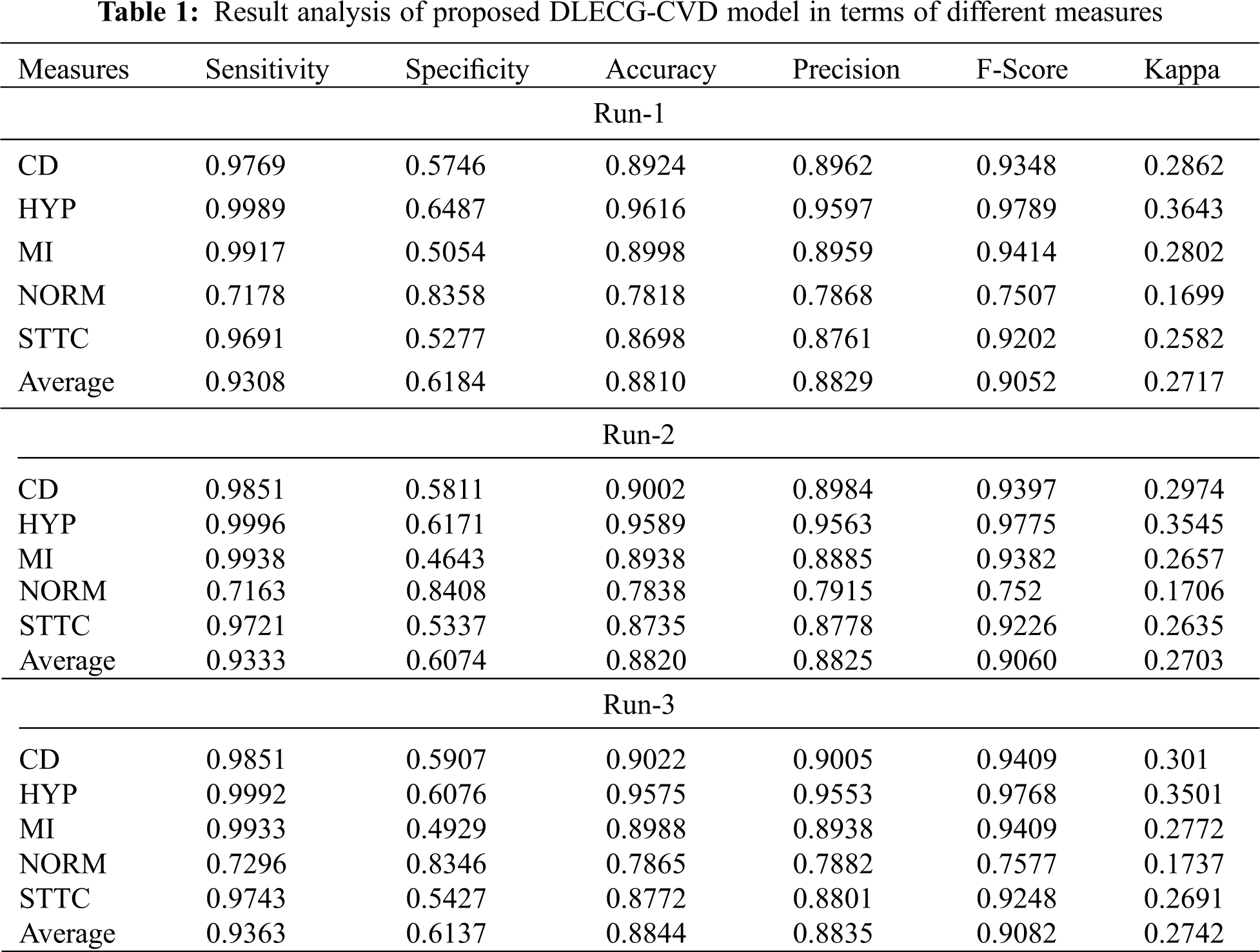
Fig. 4 depicts the ECG recognition result analysis of the DLECG-CVD model under execution run 1. The DLECG-CVD model has classified the CD class with the sens. of 0.9769, spec. of 0.5746, accuracy of 0.8924, precision of 0.8962, F-measure of 0.9348, and kappa of 0.2862. In addition, the DLECG-CVD model has classified the HYP class with the sens. of 0.9989, spec. of 0.6487, accuracy of 0.9616, precision of 0.9597, F-measure of 0.9789, and kappa of 0.3643. Also, the DLECG-CVD model has classified the MI class with the sens. of 0.9917, spec. of 0.5054, accuracy of 0.8998, precision of 0.8959, F-measure of 0.9414, and kappa of 0.2802. Additionally, the DLECG-CVD model has classified the NORM class with the sens. of 0.7178, spec. of 0.8358, accuracy of 0.7818, precision of 0.7868, F-measure of 0.7507, and kappa of 0.1699. Besides, the DLECG-CVD model has classified the STTC class with the sens. of 0.9691, spec. of 0.5277, accuracy of 0.8698, precision of 0.8761, F-measure of 0.9202, and kappa of 0.2582.
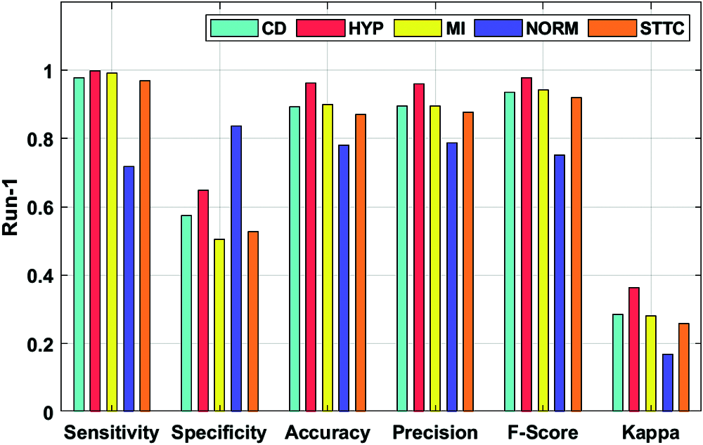
Figure 4: Result analysis of DLECG-CVD model under run-1
Fig. 5 showcases the ECG recognition outcome analysis of the DLECG-CVD model under execution run 2. The DLECG-CVD model has classified the CD class with the sens. of 0.9851, spec. of 0.5811, accuracy of 0.9002, precision of 0.8984, F-measure of 0.9397, and kappa of 0.2974. Moreover, the DLECG-CVD technique has classified the HYP class with the sens. of 0.9996, spec. of 0.6171, accuracy of 0.9589, precision of 0.9563, F-measure of 0.9775, and kappa of 0.3545. Furthermore, the DLECG-CVD approach has classified the MI class with the sens. of 0.9938, spec. of 0.4643, accuracy of 0.8938, precision of 0.8885, F-measure of 0.9382, and kappa of 0.2657. In the meantime, the DLECG-CVD model has classified the NORM class with the sens. of 0.7163, spec. of 0.8408, accuracy of 0.7838, precision of 0.7915, F-measure of 0.752, and kappa of 0.1706. At the same time, the DLECG-VD model has classified the STTC class with a sens. of 0.9721, spec. of 0.5337, accuracy of 0.8735, precision of 0.8778, F-measure of 0.9226, and kappa of 0.2635.

Figure 5: Result analysis of DLECG-CVD model under run-2
Fig. 6 portrays the ECG recognition result analysis of the DLECG-CVD technique under execution run 3. The DLECG-CVD model has classified the CD class with the sens. of 0.9851, spec. of 0.5907, accuracy of 0.9022, precision of 0.9005, F-measure of 0.9409, and kappa of 0.301. Meanwhile, the DLECG-CVD model has classified the HYP class with the sens. of 0.9992, spec. of 0.6076, accuracy of 0.9575, precision of 0.9553, F-measure of 0.9768, and kappa of 0.3501. In line with, the DLECG-CVD model has classified the MI class with the sens. of 0.9933, spec. of 0.4929, accuracy of 0.8988, precision of 0.8938, F-measure of 0.9409, and kappa of 0.2772. Simultaneously, the DLECG-CVD model has classified the NORM class with the sens. of 0.7296, spec. of 0.8346, accuracy of 0.7865, precision of 0.7882, F-measure of 0.7577, and kappa of 0.1737. Eventually, the DLECG-VD methodology has classified the STTC class with the sens. of 0.9743, spec. of 0.5427, accuracy of 0.8772, precision of 0.8801, F-measure of 0.9248, and kappa of 0.2691.
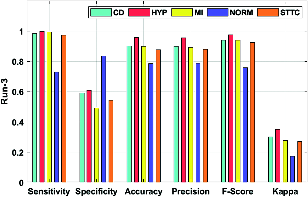
Figure 6: Result analysis of DLECG-CVD model under run-3
An average results analysis of the DLECG-CVD model on the ECG signal classification is given in Fig. 7. The DLECG-CVD model has effectively classified the ECG signals at round 1 with the maximum average sens. of 0.9308, spec. of 0.6184, accuracy of 0.8810, precision of 0.8829, F-measure of 0.9052, and kappa of 0.2717. Similarly, the DLECG-CVD model has effectively classified the ECG signals at round 2 with the maximum average sens. of 0.9333, spec. of 0.6074, accuracy of 0.8820, precision of 0.8825, F-measure of 0.9060, and kappa of 0.2703. Likewise, the DLECG-CVD model has effectively classified the ECG signals at round 3 with the maximal average sens. of 0.9363, spec. of 0.6137, accuracy of 0.8844, precision of 0.8835, F-measure of 0.9082, and kappa of 0.2742.
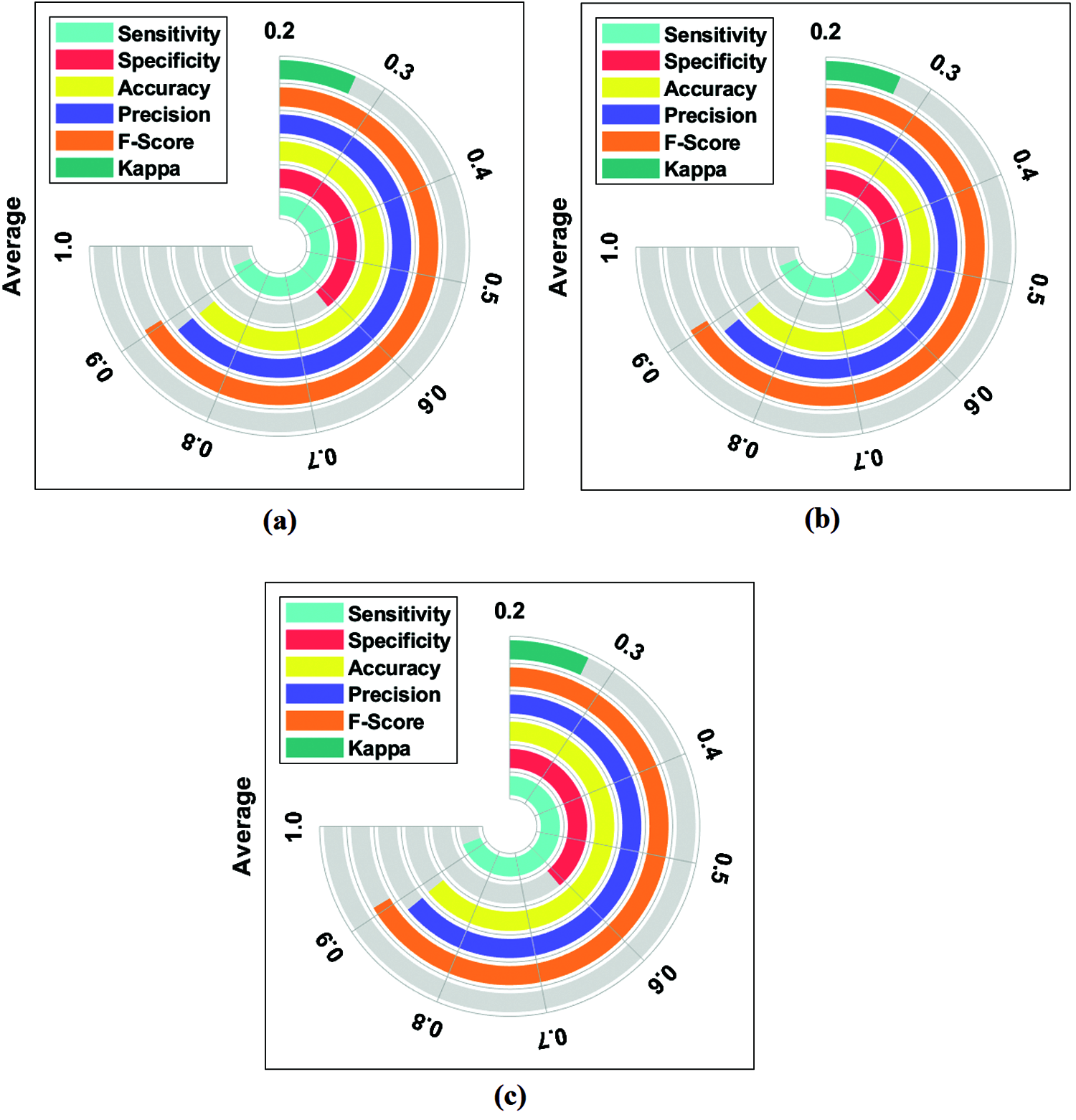
Figure 7: (a) Run-1, (b) Run-2, (c) Run-3: Average analysis of DLECG-CVD model
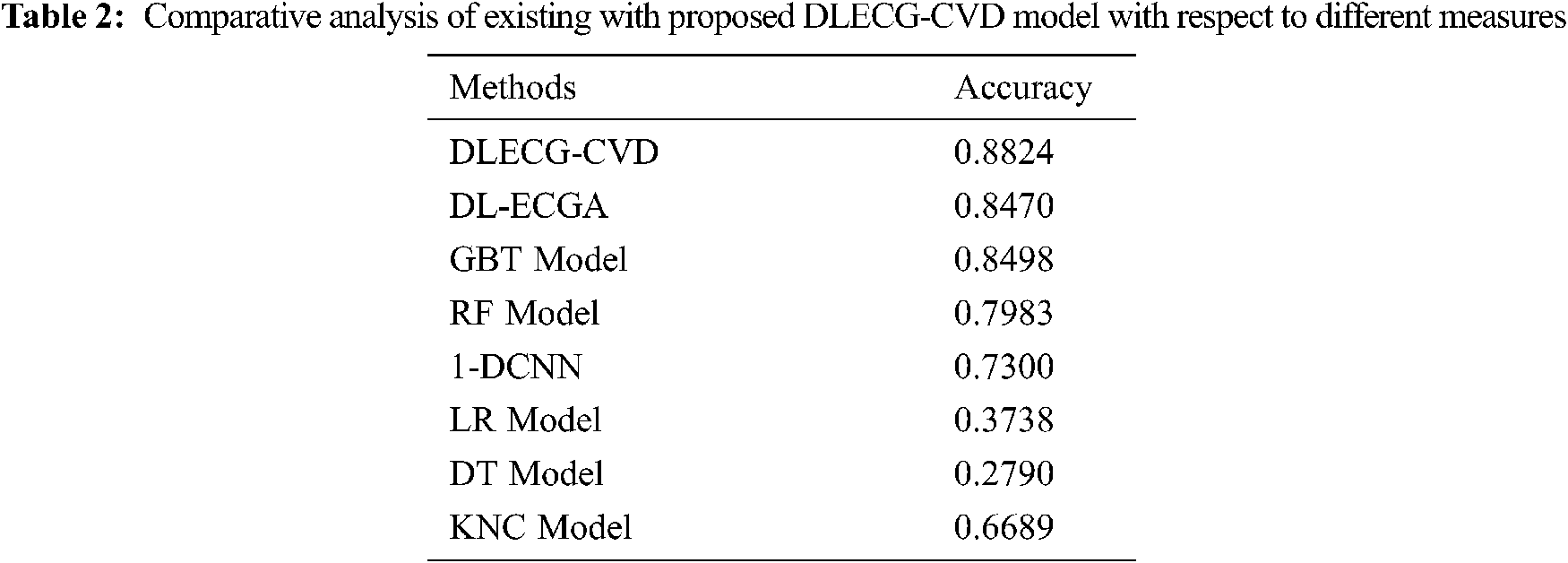
A comparative study of the DLECG-CVD model with existing techniques takes place in Tab. 2 and Fig. 8 [5]. The results showcased that the DT model has failed to show effective results with an accuracy of 0.279. Then, the LR model has attained a slightly increased result with an accuracy of 0.3738. Likewise, the KNC technique has obtained moderate performance with an accuracy of 0.6689. Afterward, the 1-DCNN and RF models have demonstrated closer results with the accuracy of 0.73 and 0.7983 respectively. Simultaneously, the DL-ECGA and GBT models have exhibited competitive accuracy values of 0.847 and 0.8498 respectively. At last, the DLECG-CVD model has outperformed the other methods with a maximum accuracy of 0.8824. Besides, the inclusion of the ISSO algorithm as a hyperparameter optimizer helps to enhance the classification performance of the DLECG-CVD model for unseen data. From the above-mentioned results, it is apparent that the DLECG-CVD model has been found to be an appropriate tool to recognize the 1D-ECG signals.
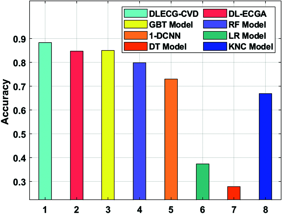
Figure 8: Accuracy analysis of DLECG-CVD model with recent methods
This paper has designed a 1-D ECG signal recognition model named DLECG-CVD. The presented model involves pre-processing, DBN based feature extraction, ISSSO based parameter tuning, and XGBoost based classification. A novel ISSO based feature selection technique is introduced by incorporating the concepts of levy flight to the SSO algorithm in order to avoid the local optima problem. Besides, the inclusion of the ISSO algorithm as a hyperparameter optimizer helps to enhance the classification performance of the DLECG-CVD model for unseen data. A detailed experimental validation process takes place using PTB-XL dataset and examined the outcomes under several dimensions. The comparative study of the DLECG-CVD model highlighted better performance over the existing techniques with the maximum accuracy of 0.8824. As a part of future scope, the performance of the DLECG-CVD model can be further increased by utilize of DL based classification models instead of XGBoost technique.
Funding Statement: The authors received no specific funding for this study.
Conflicts of Interest: The authors declare that they have no conflicts of interest to report regarding the present study.
1. M. T. Sadiq, X. Yu, Z. Yuan, Z. Fan, A. U. Rehman et al., “Motor imagery eeg signals classification based on mode amplitude and frequency components using empirical wavelet transform,” IEEE Access, vol. 7, pp. 127678–127692, 2019. [Google Scholar]
2. I. A. Doush, A. L. Quran, M. A. A. Betarand and M. A. Awadallah, “MAX-Sat problem using hybrid harmony search algorithm,” Journal of Intelligent Systems, vol. 27, no. 4, pp. 643–658, 2018. [Google Scholar]
3. M. T. Sadiq, X. Yu, Z. Yuan, F. Zeming, A. U. Rehman et al., “Motor imagery eeg signals decoding by multivariate empirical wavelet transform-based framework for robust brain–computer interfaces,” IEEE Access, vol. 7, pp. 171431–171451, 2019. [Google Scholar]
4. J. Schläpfer and H. J. Wellens, “Computer-interpreted electrocardiograms,” Journal of the American College of Cardiology, vol. 70, no. 9, pp. 1183–1192, 2017. [Google Scholar]
5. M. T. Sadiq, X. Yu and Z. Yuan, “Exploiting dimensionality reduction and neural network techniques for the development of expert brain–computer interfaces,” Expert Systems with Applications, vol. 164, pp. 114031, 2021. [Google Scholar]
6. Z. I. Attia, C. V. DeSimone, J. J. Dillon, Y. Sapir, V. K. Somers et al., “Novel bloodless potassium determination using a signal-processed single-lead ecg,” Journal of the American Heart Association, vol. 5, no. 1, pp. 1–9, 2016. [Google Scholar]
7. S. K. Lakshmanaprabu, S. N. Mohanty, S. S. Rani, S. Krishnamoorthy, J. Uthayakumar et al., “Online clinical decision support system using optimal deep neural networks,” Applied Soft Computing, vol. 81, pp. 105487, 2019. [Google Scholar]
8. J. Li, Y. Si, T. Xu and S. Jiang, “Deep convolutional neural network based ecg classification system using information fusion and one-hot encoding techniques,” Mathematical Problems in Engineering, vol. 2018, pp. 1–10, 2018. [Google Scholar]
9. K. Weimann and T. O. F. Conrad, “Transfer learning for ECG classification,” Scientific Reports, vol. 11, no. 1, pp. 5251, 2021. [Google Scholar]
10. S. K. Pandey and R. R. Janghel, “Automatic detection of arrhythmia from imbalanced ECG database using CNN model with SMOTE,” Australasian Physical & Engineering Sciences in Medicine, vol. 42, no. 4, pp. 1129–1139, 2019. [Google Scholar]
11. E. Jeon, K. Oh, S. Kwon, H. Son, Y. Yun et al., “A lightweight deep learning model for fast electrocardiographic beats classification with a wearable cardiac monitor: Development and validation study,” JMIR Medical Informatics, vol. 8, no. 3, pp. e17037, 2020. [Google Scholar]
12. A. M. Shaker, M. Tantawi, H. A. Shedeed and M. F. Tolba, “Generalization of convolutional neural networks for ecg classification using generative adversarial networks,” IEEE Access, vol. 8, pp. 35592–35605, 2020. [Google Scholar]
13. S. Nurmaini, A. Darmawahyuni, A. N. S. Mukti, M. N. Rachmatullah, F. Firdaus et al., “Deep learning-based stacked denoising and autoencoder for ecg heartbeat classification,” Electronics, vol. 9, no. 1, pp. 135, 2020. [Google Scholar]
14. J. S. Huang, B. Q. Chen, N. Y. Zeng, X. C. Cao and Y. Li, “Accurate classification of ECG arrhythmia using MOWPT enhanced fast compression deep learning networks,” Journal of Ambient Intelligence and Humanized Computing, pp. 1–18, 2020. [Google Scholar]
15. X. Han, Y. Hu, L. Foschini, L. Chinitz, L. Jankelson et al., “Deep learning models for electrocardiograms are susceptible to adversarial attack,” Nature Medicine, vol. 26, no. 3, pp. 360–363, 2020. [Google Scholar]
16. T. Wang, C. Lu, Y. Sun, M. Yang, C. Liu et al., “Automatic ECG classification using continuous wavelet transform and convolutional neural network,” Entropy, vol. 23, no. 1, pp. 119, 2021. [Google Scholar]
17. A. Peimankar and S. Puthusserypady, “DENS-Ecg: A deep learning approach for ECG signal delineation,” Expert Systems with Applications, vol. 165, pp. 113911, 2021. [Google Scholar]
18. J. Wang, X. Qiao, C. Liu, X. Wang, Y. Liu et al., “Automated ECG classification using a non-local convolutional block attention module,” Computer Methods and Programs in Biomedicine, vol. 203, pp. 106006, May 2021. [Google Scholar]
19. P. Wagner, N. Strodthoff, R. D. Bousseljot, D. Kreiseler, F. I. Lunze et al., “PTB-Xl, a large publicly available electrocardiography dataset,” Scientific Data, vol. 7, no. 1, pp. 1–15, 2020. [Google Scholar]
20. G. E. Hinton, S. Osindero and Y. -W. Teh, “A fast learning algorithm for deep belief nets,” Neural Computation, vol. 18, no. 7, pp. 1527–1554, 2006. [Google Scholar]
21. J. Yu and G. Liu, “Knowledge extraction and insertion to deep belief network for gearbox fault diagnosis,” Knowledge-Based Systems, vol. 197, pp. 105883, 2020. [Google Scholar]
22. M. Neshat, G. Sepidnam and M. Sargolzaei, “Swallow swarm optimization algorithm: A new method to optimization,” Neural Computing and Applications, vol. 23, no. 2, pp. 429–454, 2013. [Google Scholar]
23. I. Hodashinsky, K. Sarin, A. Shelupanov and A. Slezkin, “Feature selection based on swallow swarm optimization for fuzzy classification,” Symmetry, vol. 11, no. 11, pp. 1423, 2019. [Google Scholar]
24. S. K. Sarangi, R. Panda and A. Abraham, “Design of optimal low-pass filter by a new levy swallow swarm algorithm,” Soft Computing, vol. 24, no. 23, pp. 18113–18128, 2020. [Google Scholar]
25. X. Zhao, Y. Zhang, Q. Ning, H. Zhang, J. Ji et al., “Identifying N6-methyladenosine sites using extreme gradient boosting system optimized by particle swarm optimizer,” Journal of Theoretical Biology, vol. 467, pp. 39–47, 2019. [Google Scholar]
 | This work is licensed under a Creative Commons Attribution 4.0 International License, which permits unrestricted use, distribution, and reproduction in any medium, provided the original work is properly cited. |