DOI:10.32604/csse.2022.022314
| Computer Systems Science & Engineering DOI:10.32604/csse.2022.022314 | |
| Article |
Make U-Net Greater: An Easy-to-Embed Approach to Improve Segmentation Performance Using Hypergraph
1Chengdu Institute of Computer Application, University of Chinese Academy of Sciences, Chengdu, 610041, China
2School of Computer Science, Chengdu University of Information Technology, Chengdu, 610225, China
3University of Chinese Academy of Sciences, Beijing, 100049, China
4Department of Experimental Rheumatology, Nijmegen, 6525GA, Netherlands
*Corresponding Author: Zhe Cui. Email: cuizhe@casit.com.cn
Received: 02 August 2021; Accepted: 03 September 2021
Abstract: Cardiac anatomy segmentation is essential for cardiomyopathy clinical diagnosis and treatment planning. Thus, accurate delineation of target volumes at risk in cardiac anatomy is important. However, manual delineation is a time-consuming and labor-intensive process for cardiologists and has been shown to lead to significant inter-and intra-practitioner variability. Thus, computer-aided or fully automatic segmentation methods are required. They can significantly economize on manpower and improve treatment efficiency. Recently, deep convolutional neural network (CNN) based methods have achieved remarkable successes in various kinds of vision tasks, such as classification, segmentation and object detection. Semantic segmentation can be considered as a pixel-wise task, it requires high-level abstract semantics information while maintaining spatial detail contexts. Long-range context information plays a crucial role in this scenario. However, the traditional convolution kernel only provides the local and small size of the receptive field. To address the problem, we propose a plug-and-play module aggregating both local and global information (aka LGIA module) to capture the high-order relationship between nodes that are far apart. We incorporate both local and global correlations into hypergraph which is able to capture high-order relationships between nodes via the concept of a hyperedge connecting a subset of nodes. The local correlation considers neighborhood nodes that are spatially adjacent and similar in the same CNN feature maps of magnetic resonance (MR) image; and the global correlation is searched from a batch of CNN feature maps of MR images in feature space. The influence of these two correlations on semantic segmentation is complementary. We validated our LGIA module on various CNN segmentation models with the cardiac MR images dataset. Experimental results demonstrate that our approach outperformed several baseline models.
Keywords: Convolutional neural network; semantic segmentation; hypergraph neural network; LGIA module
Heart disease is one of the most serious causes of sudden death. The number of sudden deaths caused by heart disease increases year by year. In routine heart disease diagnosis, treatment planning and prognostic estimation, cardiologists are required to delineate the myocardium outline. However, manual delineation is a time-consuming and labor-intensive process for cardiologists and has been shown to lead to significant inter-and intra-practitioner variability. To improve efficiency and accuracy, clinicians often use computer-aided tools [1] to fulfill the segmentation task. In this regard, fully computer-aided diagnosis systems are highly desirable.
In recent years, deep convolutional neural networks (CNNs) make remarkable achievements in various computer vision tasks, such as classification [2–4], [5,6], semantic segmentation [7–9], object detection [10–13], and object tracking [14,15]. Different from the image classification task which assigns category labels for the whole image, the semantic segmentation task is required to predict the category label of each pixel in an image. Large receptive field size is a necessary factor to understand the scene context and the essential prerequisite to the success of various vision tasks. To achieve good performance, traditional CNNs generally stack pooling layers and striding convolution layers to obtain a large receptive field size. Unfortunately, the semantic segmentation task needs preserving of the spatial size, which is a natural contradiction between high-level semantic and fine space details.
More frustratingly, too many down-sampling operators will significantly reduce the spatial size of the feature map. The segmentation task requires getting a size-equal mask as the original image, so the reduction in spatial size is catastrophic. Fully Convolutional Networks (FCN) [7] popularized CNN architectures for dense predictions without any fully connected layers. It is an end-to-end network and can accept input images of different sizes without requiring all training images and test images to have the same size [16]. FCN attempts to recover the category to which each pixel belongs from the abstract features. That is, further extend the image level classification to the pixel level classification. However, each pixel is classified without considering the relationship between pixels, ignoring the spatial regularization steps used in the segmentation method based on the pixel classification, and lacking spatial consistency. Encoder-decoder architectures like U-net [8] are state-of-art methods for pixel-wise prediction tasks in the computer vision field. U-net is based on FCN and is a full-convolution network that replaces a fully connected layer with a convolutional layer. It combines the feature of each upsampling layer with the features of the corresponding downsampling layer. Both FCN and U-net can only bring about a linear growth of the receptive field size.
To gain a larger feature map spatial resolution meanwhile providing a larger receptive field size, the atrous convolution [17] was used in later CNN networks. The difference between the atrous convolution kernel and the traditional convolution kernel is that the atrous convolution introduces the concept of dilated rates into the convolution filter template. By inserting a varied number of zero values between positions of successive filter value, atrous convolution can prompt neurons to have larger receptive field sizes than traditional convolution at the same downsampling rate. It seems that using larger dilated rates can bring a larger receptive field size at the same feature map spatial resolution. This way can bring about the exponential growth of the receptive field size. Unfortunately, as the dilated rate continues to increase, especially beyond 24, the atrous convolution gradually loses its effectiveness and results in a decline in performance [18].
Graph-based methods [19,20] have attracted much attention because of their ability to directly capture the connections between objects. This allows us to alleviate the contradiction between high-level semantic and fine space details mentioned below. However, the majority of these works are based on modeling the pair-wise relationships between samples, failing to capture their higher-order relationships. Hypergraph Neural Networks (HGNN) [21] enables us to more directly implement the requirements of relation modeling across long spatial distances. The network utilizes a hypergraph structure for data relational modeling. The main difference between a traditional graph and a hypergraph is that graphs are only able to represent one-to-one node relationships via edges while hypergraphs can capture high-order relationships between nodes via the concept of a hyperedge connecting a subset of nodes. A hyperedge links one central node and its neighbors according to the similarity relationship on the graph.
In this paper, we propose an easy-to-embed module aggregating both local and global information (aka LGIA module) to capture the high-order relationship between nodes that are far apart. It can be integrated into ready-made CNN-based segmentation models to improve baseline models, such as U-Net and FCN on medical image datasets. Inspired by the recent success of CNN segmentation networks and popular graph-based methods, our LGIA module exploits hypergraph convolutional layers to capture both short-range and long-range contextual information respectively for semantic segmentation. High-level semantic information is indispensable for the correct identification of objects. To obtain higher-level information, the model adopts a larger receptive field size to make the neurons look wider and facilitates long-range interactions. The overview of our proposed method is illustrated in Fig. 1. The LGIA module is applied to the traditional CNN-based model for left ventricular myocardium segmentation. Here the traditional CNN-based model consists of an encoder and decoder. A hypergraph is constructed according to CNN encoder feature maps, and the feature maps processed by hyperedge convolutions continue to be input into the CNN decoder. The two main key contributions of this paper are as follows:
(1) We propose an easy-to-embed module (LGIA module) which can be inserted into existing CNN-based models like U-Net and FCN, and models both local and global context information efficiently to improve semantic segmentation performance.
(2) We employ HGNN to get both local and global information aggregation graph which is beneficial to semantic segmentation. Both closeness in spatial distance and feature activation distance is exploited to achieve this aggregation.
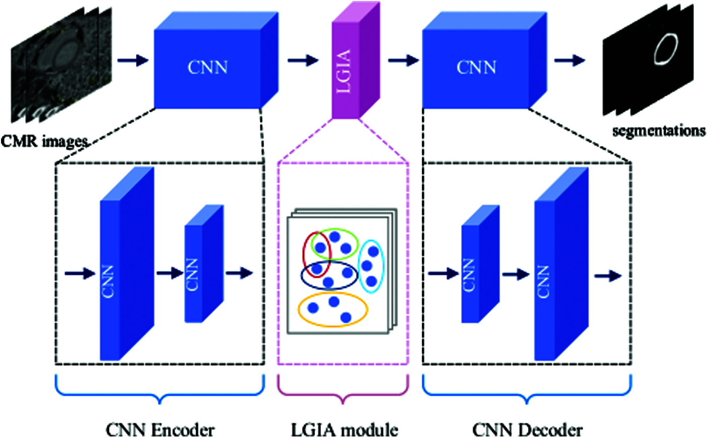
Figure 1: Overview construction of the proposed plug-and-play LGIA module
CNN-based methods have achieved extraordinary performance in numerous computer vision tasks in recent years. From AlexNet [2], VGGNet [3] to ResNet [4] and Xception [22], the object recognition score records are constantly refreshed in various classification tasks. The CNN models take advantage of convolution layers and pooling layers to continuously concentrate implicit knowledge to obtain feature maps that contain dense and abstract semantic information. With CNN architectures, models have powerful feature representation ability, can accurately identify the semantic information in the image in an end-to-end manner. Semantic segmentation is another fundamental task related to classification, but it is more challenging. Segmentation aims at producing a label mask of all pixels and therefore it can be regarded as a pixel-wise classification. More particularly, the segmentation problem can be solved by classifying each pixel of an image into different object categories.
2.1 Patch-Based Semantic Segmentation Methods
One of the popular initial deep learning approaches is patch classification where each pixel is separately classified using a patch of the image around it. The main reason to use patches is that classification networks usually have full connected layers and therefore require fixed-size images. Moreover, a single pixel only contains very limited information, especially the one-channel grayscale medical image. Consequently, many segmentation methods [23–25] use image patches instead of pixels as network input. In the training phase, several patches are extracted randomly from images, and overlap is allowed between patches. The method regards the label of the patch center pixel as the label of this patch. All the patches and the corresponding labels obtained from ground-truth are composed of training sets, which are input into the CNN network for training. In the reasoning stage, the method thinks of each pixel as a patch center, continuously and closely extracting the patches represented by all the pixels in the image. And the classification model infers the label of each patch representing a pixel for prediction on the testing dataset. The classification model generates the pixel-wise segmentation probability response map by inferring the label of each patch. Patch-based methods can only see limited local pixels and can't learn the relationship between objects from remote context information.
2.2 FCN-Based Semantic Segmentation Methods
Image-based methods are proposed to solve the drawback of pixel-based or patch-based methods. Recently advanced segmentation networks are inspired by the fully convolutional network (FCN) [7]. Compared to a patch-based CNN for segmentation, FCN takes full images as input and yields a size-equal prediction mask as the original image. This allows segmentation maps to be generated for an image of any size and was also much faster compared to the patch classification approach. This end-to-end training and testing fashion are widely adopted by later works, such as U-Net [8]. These methods have been successfully applied on many pixel-wise prediction tasks and usually consist of two parts, encoder and decoder [26,27]. The encoder adopts CNN as the backbone which cascades striding convolution layers and pooling layers to extract high-level representations from the original image. The decoder adopts transposed convolution [28] to recover precise localization information by gradually applying up-sampling. Since up-sampling is a sparse operation and always causes spatial distortion, the U-Net designs skip connection to concatenate the high-resolution but poor-semantic feature maps from the decoder to the low-resolution but rich-semantic feature maps from the decoder to learn better spatial location information. The large receptive field is the key factor to achieve high segmentation performance, hence the encoder stacks convolutional components to gain receptive fields. Unfortunately, stacked convolutional components can only lead to the linear growth of the receptive fields. DeepLab series [9,17,18,29] relieve this obstacle by adopting atrous convolutions and atrous spatial pyramid pooling (ASPP).
2.3 Graph Convolutional Networks
Many methods can utilize a graph to achieve reliable performance in various fields. Graph Convolution Networks (GCN) [19] are proposed for semi-supervised classification on graph-structured data. The graph-based method shows the promise of the modeling ability of the relationship between objects. Unlike standard convolutions, GCNs learn with a graph that can be represented using the adjacency matrix. The graph-based method CRFs [30] are proposed to apply in the image segmentation task. And the DeepLab v1 [9] also uses fully connected CRFs as a part of the model. Gadde et al. introduced a bilateral inception module [31] that can be inserted in existing CNN architectures for semantic image segmentation. Gao et al. [32] proposed Graph U-Net (GUnet) which applies an encoder-decoder architecture leveraging graph convolution and it improves on GCN by generalizing the seminal U-Net designed for Euclidean spaces to non-Euclidean spaces, allowing high-level feature encoding and receptive field enlargement through the sampling of important nodes in a graph. Different from the graph, the hypergraphs can connect multiple nodes with one hyperedge, this can represent more complex relationships than a graph. Another difference is that hypergraphs can be described by the incidence matrix which is composed of the relationship between vertexes and edges. This feature makes hypergraph easier to expand by combining multiple matrices. Yadati et al. [33] applied Hypergraph Convolutional Networks (HyperGCN) to the problem of semi-supervised learning (SSL) on attributed hypergraphs. Lostar et al. [34] proposed the Hypergraph U-Net (HUNet) architecture for high-order data embedding by generalizing the graph U-Net [32] to hypergraphs. Jin et al. [35] proposed a hypergraph induced Convolutional Manifold Networks (H-CMN) which was efficient for the large-scale dataset. They define convolutions over super-pixels by defining connectivity among them.
In this section, we introduce our proposed LGIA module which can be easily embedded into current CNN image semantic segmentation models. Consider given gray-scale MR image
In traditional graph convolutional neural network methods, the pairwise connections among data are employed [21]. However, the data structure in real practice could be beyond pairwise connections and even far more complicated. Compared with the traditional graph which only connects two nodes with one edge, the hypergraph can include more than two nodes within a hyperedge. Therefore, hypergraphs can model more complex relations among data beyond pairwise connections.
A hypergraph can be defined as
where a vertex v belongs to vertex set V, and an edge
With the hypergraph incidence matrix
where the
In our experiments, images in the dataset are all gray-scale with only a single scalar. Consequently, due to the lack of enough semantic information, it is not recommended to use information from the shallow stage as a node for hyperedges constructing. The high-level semantic features which are produced from a series of convolution layers and pooling layers are employed in our hyperedge construction strategy. As deeper layers gain greater receptive field size, the output feature maps contain more advanced abstractions in both feature dimensions and spatial dimensions. The reduced size feature map encodes the hidden information of the original large size image, which not only provides a reliable basis for us to find the similarity among nodes but also facilitates the modeling of the relationship between objects across a distant range.
Our proposed LGIA module is illustrated in the middle of Fig. 2. There are two hyperedge construction schemes are adopted, local and global. Each node is selected as the central node (yellow block) in both schemes, then K nodes (red block) closest to it are found to form a hyperedge. In the local scheme, the K nodes are chosen from the 8-connected coordinate space. In the global scheme, the K nodes are selected from all feature maps in one batch of feature space. The LGIA module consists of two hyperedge convolution layers, and each convolution layer is followed by a nonlinear activation function and a dropout. The first hyperedge convolution layer takes C1 channels as input which equals the channel of CNN feature map, and output feature maps with C2 channels which are defined as the dimension of the hidden layer. And the second hyperedge convolution layer takes feature maps with C2 channels then produces C3 channels which are required by the following CNN layers.
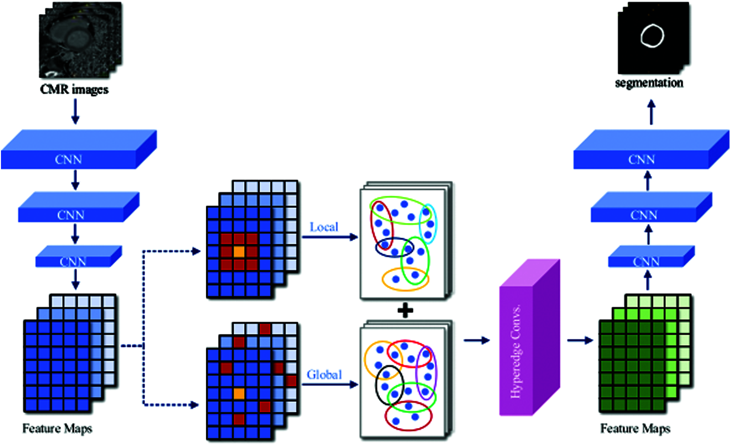
Figure 2: Overview of CNN segmentation architecture with embedded LGIA module
The LGIA module takes a batch of feature maps with the shape of
3.3 Local and Global Information Aggregation
Traditional CNNs focus only on local features and ignore global region features, which are both important for pixel classification and recognition [36]. Hypergraph allows a more direct way to model these local and global connections. In this method, we use hypergraph to integrate local and global correlation in coordinate space and feature space straightforwardly. Each node contains its own attributes, and each hyperedge contains numerous nodes with some correlation according to the correlation between each other. K Nearest Neighbors (KNN) is one of the most commonly used methods for building hyperedge. In this way, a hyperedge will contain the most similar K nodes of the central node on a kind of measure. The correlation between nodes will be enhanced by the information aggregation of hyperedge.
In our proposed method, there are two modes of hyperedges constructing methods, they are the relationship in local coordinate space and the relationship in global feature space. These two modes of hyperedges could be represented as two hypergraph incidence matrixes which are subsequently concatenated to one incidence matrix
3.3.1 Neighbors in Local Coordinate Space
Because of the local self-similarity of images, pixels adjacent to one pixel are quite potential belong to the same category of object. The adjacent context information around the center pixel can be used to infer the current category. Local similarity theory exists in both low-level and high-level feature maps. Therefore, we need to model the local similarity relationship.
To achieve this goal, an 8-connected nearest neighbor relationship in coordinate space is adopted. Each hyperedge contains eight nodes that are connected to the central node horizontally, vertically, and diagonally. This natural spatial neighborhood information of objects is conducive to the correct classification of objects. Note that the nodes on the four boundaries of the image have incomplete adjacent nodes, and there are only three adjacent nodes of the four corners nodes. With the flexibility of hyperedge, a varying number of nodes can be connected.
3.3.2 Neighbors in Global Feature Space
The relationship between objects in long-distance is the key to success for correct segmentation which can be considered as pixel-level classification.
To explore the association between objects in the global scope, we introduce the similarity on the whole batch of feature maps. In general, KNN is often used to select nodes with similar features. The feature maps operated by convolution filters repeatedly have fewer noisy and higher semantic. Furthermore, the size of reduced feature maps can characterize high-resolution features with dense information. In this manner, each hyperedge contains Kglobal nearest neighbor nodes from each feature map in one batch, and the similarity is measured by Euclidean distance between the central.
The plug-and-play module we proposed consists of two hyperedge convolution layers. The first hyperedge convolution layer takes features with the input dimension as the output of the upper layer CNN and turns out a feature map with the acceptance dimension of the latter CNN layer. The last hyperedge convolution layer takes the output feature map of the previous layer as input. In order to reduce overfitting, we use a drop layer with p = 0.2 to follow each hyperedge convolution layer. To obtain nonlinearly, we choose Leaky ReLU [37] as the activation function for each hyperedge convolution layer.
In our experiments, U-Net [8] and FCN [7] with three times downsampling are selected for the control experiments. We replace the proposed LGIA module with the shallow, deep, and bottleneck layers of the CNN segmentation network to explore its impact on performance with the position. During the training phase, Adam optimizer [38] with a base learning rate value of 5e−3 is used to minimize the Cross-Entropy loss function. The proposed method is implemented with the PyTorch library [29] and trained from scratch for 300 epochs. Then test on randomly selected 10% of the datasets.
To illustrate the effectiveness of our proposed method, we conduct experiments of different methods on the same dataset with equivalent experimental conditions and same post-processing. Comparison methods include advanced CNN-based segmentation models U-Net and FCN.
Our dataset contains Cardiac Magnetic Resonance (CMR) images from 80 different patients with cardiomyopathy. All images are 2D short-axis native T1 mapping CMR images [39]. The spacing size of those images is range from 1.172 × 1.172 × 1.0 mm3 to 1.406 × 1.406 × 1.0 mm3. The original spatial dimension of those images is 256 × 218 × 1 pixels.
In order to ensure the isotropy of data in each dimension, we use the interpolation method to re-sample the spacing size to 1.0 × 1.0 × 1.0 mm3. Because a CMR image contains a wide scan range of chest, we crop and resize the image to 80 × 80 based on the consideration of computational efficiency and space utilization. Since the large range of grayscale in the CMR image, we normalize each CMR image to ensure intensities range of [−1.0, 1.0] for efficiently processing by the deep model.
In order to evaluate the network performance objectively and quantitatively, we investigated a variety of evaluation indicators. And Dice Similarity Coefficient (DSC) [40] is widely used to evaluate the accuracy of segmentation methods. The DSC is defined as Eq. (3):
where
In this part, we conduct several sets of ablation studies about our proposed LGIA module and considering four scenarios: 1) which position of CNN segmentation network will LGIA module be embedded in; 2) K value in the hyperedge construction strategy should be chosen; 3) how many hyperedge convolution layers does LGIA module consist of; 4) how the performance varies with only the local block and only the global block. Then, different CNN segmentation networks are adopted for further experiments to verify the effectiveness and reliability of the proposed LGIA module.
5.3.1 Embedded Position of LGIA Module
CNN repeatedly stacks the pooling layers and striding convolution layers to obtain a larger receptive field size, which results in a progressively shrinking size of feature maps. The shallow layers in CNNs are more concentrated on learning low-level features, like object edges and curves. The feature maps in shallower layers are richly detailed but poorly semantic. Instead, the feature maps in deeper layers are richly semantic but poorly detailed. Feature maps in different network stages contain various information, so the hypergraphs constructed above are not identical. In order to explore the impact of this difference on the segmentation performance, we conduct experiments that use dissimilar feature maps from different network stages as LGIA module inputs. Feature maps with the too-small resolution are count against to hypergraph construction, so we adopt 3 max-pooling layers in U-Net and FCN to avoid oversized resolution reduction caused by excessive downsampling operations. Therefore, the size of feature maps is reduced by up to 8 times compared with the original image size.
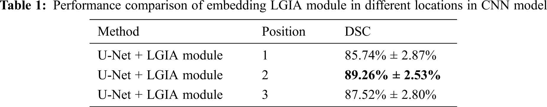
For the convenience of description, we number different possible embedded locations in the original CNN network. In U-Net experiments, we embed the LGIA module in the shallow and deep stages of the encoder, and the deep stage of the decoder respectively. We define shallow encoder embedded location (position 1) as in front of the first pooling layer, the shape of the feature maps fed in LGIA module here is (Batch Size, 1,
The results of embedded positions are illustrated in Tab. 1. In this embedding position experiment, the number of hyperedge convolution layers is 2, and the Kglobal value is 9. The observations support that the segmentation performance improvements achieved by embedding the LGIA module in the deep stage of the CNN model. From the results in the table, we can further investigate that when embedded in the shallow encoder layer (position 1), deep encoder stage (position 2) and deep decoder stage (position 3) of U-Net, 85.74% ± 2.87%, 89.26% ± 2.53% and 87.52% ± 2.80% DSC values are obtained respectively. The worst results are obtained when embedded in the shallow encoder layer (position 1) because the input images of the LGIA module in this layer are not smooth enough and contains a lot of noise, which will result in an inaccurate hypergraph being created. The best results are obtained when embedded in the deep encoder stage (position 2) because the input feature maps of the LGIA module in this stage are noise-free and richly semantic. In addition, it is easier to model long-distance relationships by constructing a hypergraph in these reduced feature maps.
5.3.2 K Value in Hyperedge Construction Schemes
For the ordinary graph, each edge connects two nodes. This can be formed by selecting one node as the central node and then looking for another node that is most similar to it. But for hypergraph, one of the most significant differences is that each edge in hypergraph (called hyperedge) will link more than two nodes. A hyperedge consists of one selected central node and its K nearest neighbors.
In our experiments, two hyperedge construction schemes are adopted, local and global. The local hyperedge construction strategy according to the 8-connected in coordinate space of each central node. In this mode, each hyperedge connects eight nodes, the Klocal = 8. For the global hyperedge construction strategy, the K nearest neighbors are selected by the similarity with the central node in feature space. In practice, we choose the most similar first k nodes. In order to explore the influence of Kglobal in global hyperedge construction strategy on the performance, we conducted experiments that adopt 5, 7, 9, 11, 13 and 15 layers when choosing the most similar first k nodes.
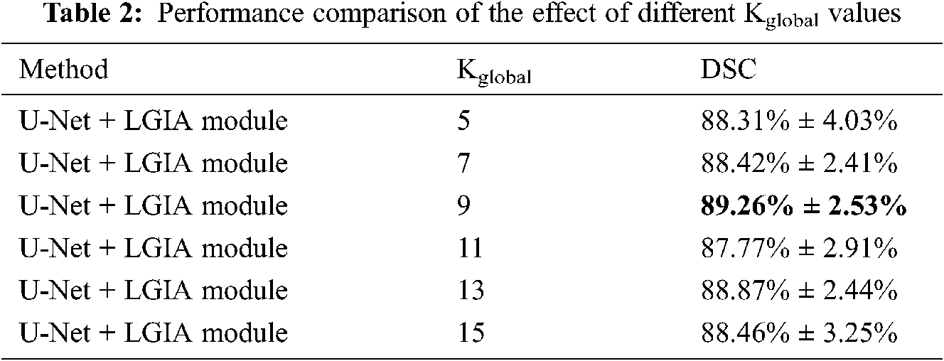
The results of the influence of the Kglobal value are shown in Tab. 2. In this Kglobal value experiment, the embedding position is 2, and the number of hyperedge convolution layers is 2. Detailed results are that adopt 5, 7, 9, 11, and 13 of the Kglobal value in global hyperedge construction strategy, 88.31% ± 4.03%, 88.42% ± 2.41%, 89.26% ± 2.53%, 87.77% ± 2.91%, 88.87% ± 2.44% and 88.46% ± 3.25% DSC values are obtained, respectively. We can observe that as the Kglobal value increases from 5 to 9, the model reports better results, but as the Kglobal value continues to increase, the performance has declined. The best result was obtained at Kglobal = 9.
5.3.3 The Number of Layers of the LGIA Module
The deeper CNN has stronger representation capabilities. But the problem of the vanishing gradients once hindered the development of technology and the improvement of performance until the appearance of ResNet [4]. Features can be performed node-edge-node transformed by hyperedge convolution operation, with a hypergraph structure that can perform better aggregate information and refine features. Using fewer hyperedge convolutional layers will result in weak describing ability. But stacking too many hyperedge convolutional layers can cause the gradient to disappear. The excessive propagation on hypergraph will reach the state of over-smoothing, which will eventually lead to the convergence of the graph vertices features [41]. Like most state-of-the-art GCNs, models generally have no more than 4 layers [42].
In order to explore the influence of the number of hyperedge convolutional layers in the LGIA module on the performance, we conducted experiments that adopt 1–4 layers in the LGIA module.
The results of the influence of hypergraph convolution layers are shown in Tab. 3. In this number of hyperedge convolution layers experiment, the embedding position is 2, and the Kglobal value is 9. We can notice that adopt 1–4 hyperedge convolutional layers in LGIA module, 87.71% ± 2.87%, 89.26% ± 2.53%, 88.49% ± 2.74% and 88.62% ± 3.77% DSC values are obtained, respectively.
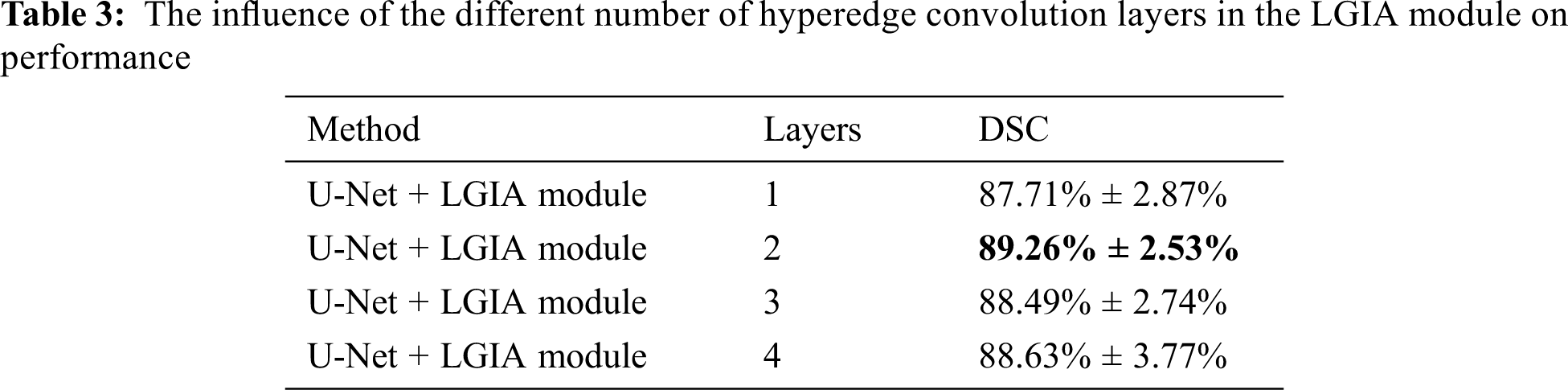
When there is only one hyperedge convolutional layer in the LGIA module, the model reported a poor score. Because it is not powerful enough in parameter quantity and representation ability. The best results are brought out by the two layers of the LGIA module. At this point, the network has enough parameter quantities to fit data patterns, and it can also effectively perform information aggregation. However, when the LGIA module depth continues to increase to 4, the performance will not increase but will decrease slightly. This is consistent with previous researches that too deep a network structure is likely to lead to vanishing gradients.
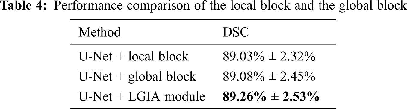
5.3.4 Effectiveness of Local or Global Aggregation
In order to explore the performance of the local or global block in the LGIA module on the performance, we conducted experiments that adopt local block only and global block only in the LGIA module.
The results of the influence of local and global blocks are shown in Tab. 4. In this local and global block experiment, the embedding position is 2, the number of hyperedge convolution layers is 2, and the Kglobal value is 9. We can notice that adopt local and global blocks only in the LGIA module, 89.03% ± 2.32% and 89.08% ± 2.45% DSC values are obtained, respectively. When we adopt the LGIA module which contains local and global blocks, the DSC value is 89.26% ± 2.53%.
5.4 Experimental Results
In this part, we present our segmentation performance comparisons with vanilla CNN-based segmentation models and the models after the insertion of our proposed LGIA module. In these controlled experiments, the network configuration and experimental conditions are all the same except whether the LGIA module is embedded or not.
In order to visually illustrate the effectiveness of our proposed LGIA module, we visualized the error analysis map of the segmentation masks.
In Fig. 3, there are three examples of the qualitative segmentation error analysis results are shown. Columns from left to right: original MR images, ground-truth, segmentation results by U-Net, segmentation results by U-Net + LGIA module. The color representation of the last two columns: blue: correct pixels, red: unidentified pixels, green: misidentified pixels. According to the color identifications in the figure, we can observe that the segmentation masks have a more correctly segmented area and less mistakenly segmented pixels after applying the LGIA module. Thus, compared to vanilla U-Net, the model with embedded LGIA module archive better results, which are closer to manual ground truth.
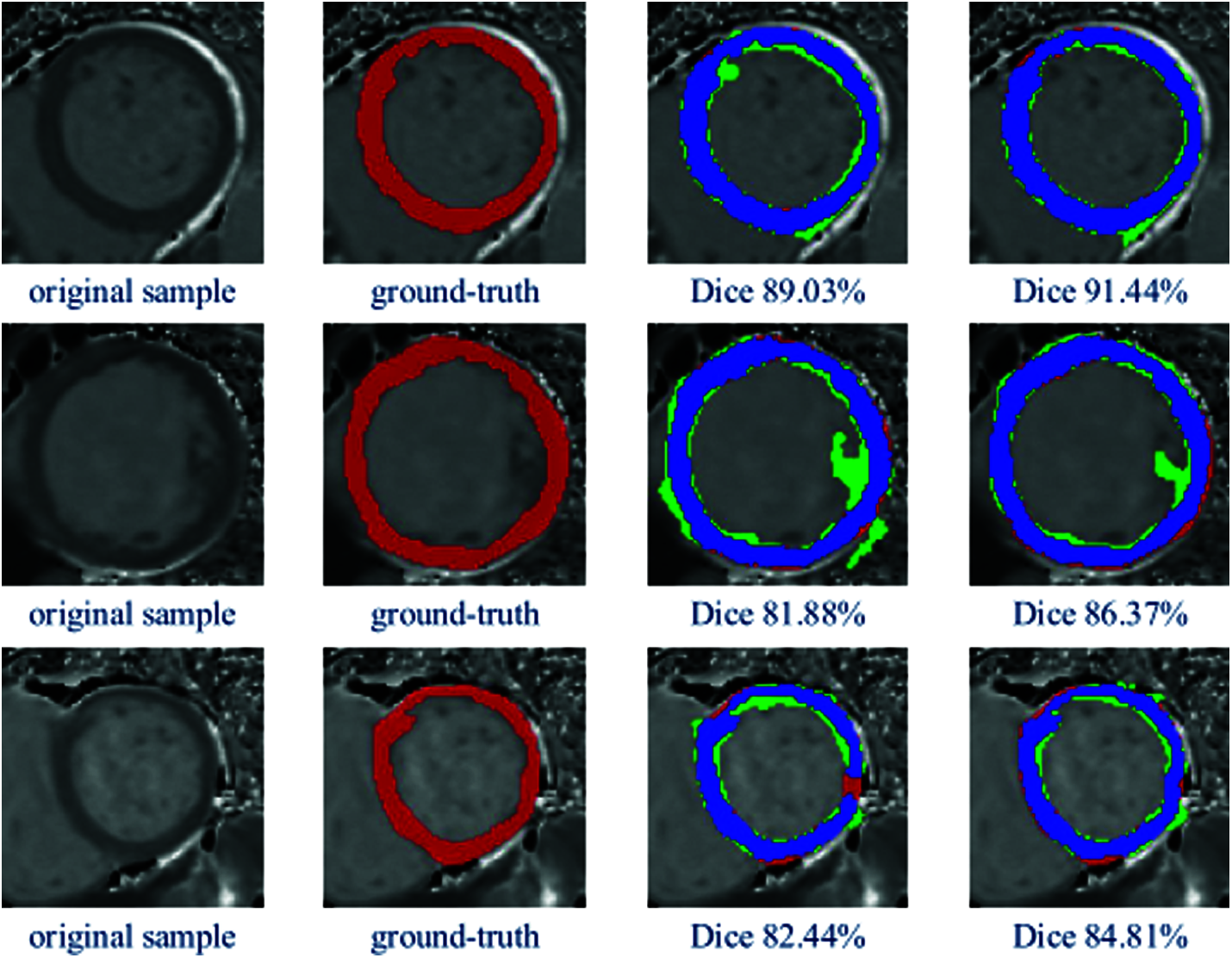
Figure 3: Examples of qualitative segmentation comparison
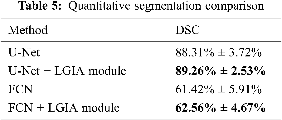
The performance of our approach has been qualitatively illustrated through error analysis maps. To make a more precise and objective demonstration of the effectiveness of our proposed method, we compare baseline models and the models after the insertion of our proposed LGIA module in terms of the DSC metric with the same training set.
The comparison results are shown in Tab. 5. We compared U-Net and FCN after embedding the LGIA module. Average scores with standard deviation on the testing set are reported. After using our proposed LGIA module, the modified models reached about 1% increasing compared to the original models.
In this paper, we proposed an easy-to-embedded block to improve segmentation performance based on the hypergraph neural network. The fundamental idea is to model the global context in the segmentation task. Most traditional CNN networks are trying to increase the receptive field size by stack string layers or using dilated Convolution. Unfortunately, this is an inefficient way because the receptive field size grows slowly. In addition, there is a contradiction that excessive downsampling operations will also cause loss of resolution, while the segmentation task requires models of product equal-sized masks.
Our proposed LGIA module takes advantage of the hypergraph to achieve local and global information aggregation. Beyond that, our approach as a stand-alone module can be embedded into existing segmentation networks without pain.
Acknowledgement: The authors would like to thank all participants for their valuable discussions regarding the content of this article.
Funding Statement: This work was supported by the Sichuan Science and Technology Program (Grant No. 2019ZDZX0005, 2019YFG0496, 2020YFG0143, 2019JDJQ0002 and 2020YFG0009).
Conflicts of Interest: The authors declare that they have no conflicts of interest to report regarding this study.
1. P. V. Tran, “A fully convolutional neural network for cardiac segmentation in short-axis MRI,” in Proc. of the IEEE Conf. on Computer Vision and Pattern Recognition (CVPR), Boston, USA, pp. 1–21, 2016. [Google Scholar]
2. A. Krizhevsky, I. Sutskever and G. E. Hinton, “ImageNet classification with deep convolutional neural networks,” Advances in Neural Information Processing Systems, vol. 25, no. 2, pp. 1–9, 2012. [Google Scholar]
3. K. Simonyan and A. Zisserman, “Very deep convolutional networks for large-scale image recognition,” in Proc. of the Int. Conf. on Learning Representations (ICLRSan Diego, USA, pp. 1–14, 2015. [Google Scholar]
4. K. M. He, X. Y. Zhang, S. Q. Ren and J. Sun, “Deep residual learning for image recognition,” in Proc. of the IEEE Conf. on Computer Vision and Pattern Recognition (CVPRLas Vegas, USA, pp. 770–778, 2016. [Google Scholar]
5. C. Szegedy, W. Liu, Y. Q. Jia, P. Sermanet, S. Reed et al., “Going deeper with convolutions,” in Proc. of the IEEE Conf. on Computer Vision and Pattern Recognition (CVPRBoston, USA, pp. 1–9, 2015. [Google Scholar]
6. H. Wu, Q. Liu and X. Liu, “A review on deep learning approaches to image classification and object segmentation,” Computers, Materials & Continua, vol. 60, no. 2, pp. 575–597, 2019. [Google Scholar]
7. J. Long, E. Shelhamer and T. Darrell, “Fully convolutional networks for semantic segmentation,” in Proc. of the IEEE Conf. on Computer Vision and Pattern Recognition (CVPRBoston, USA, pp. 3431–3440, 2015. [Google Scholar]
8. O. Ronneberger, P. Fischer and T. Brox, “U-net: Convolutional networks for biomedical image segmentation,” in Int. Conf. on Medical Image Computing and Computer-Assisted Intervention (MICCAIMunich, Germany, pp. 234–241, 2015. [Google Scholar]
9. L. C. Chen, G. Papandreou, L. Kokkinos, K. Murphy and A. L. Yuille, “Semantic image segmentation with deep convolutional nets and fully connected CRFs,” in Proc. of the Int. Conf. on Learning Representations (ICLRSan Diego, USA, pp. 1–14, 2015. [Google Scholar]
10. R. Girshick, J. Donahue, T. Darrell and J. Malik, “Rich feature hierarchies for accurate object detection and semantic segmentation,” in Proc. of the IEEE Conf. on Computer Vision and Pattern Recognition (CVPRColumbus, USA, pp. 580–587, 2014. [Google Scholar]
11. J. Redmon, S. Divvala, R. Girshick and A. Farhadi, “You only look once: Unified, real-time object detection,” in Proc. of the IEEE Conf. on Computer Vision and Pattern Recognition (CVPRLas Vegas, USA, pp. 779–788, 2016. [Google Scholar]
12. W. Liu, D. Anguelov, D. Erhan, C. Szegedy, S. Reed et al., “SSD: Single shot multibox detector,” in Proc. of the European Conf. on Computer Vision (ECCVAmsterdam, Netherlands, pp. 21–37, 2016. [Google Scholar]
13. C. Song, X. Cheng, Y. X. Gu, B. J. Chen and Z. J. Fu, “A review of object detectors in deep learning,” Journal on Artificial Intelligence, vol. 2, no. 2, pp. 59–77, 2020. [Google Scholar]
14. Z. T. Li, W. Wei, T. Z. Zhang, M. Wang, S. J. Hou et al., “Online multi-expert learning for visual tracking,” IEEE Transactions on Image Processing, vol. 29, pp. 934–946, 2020. [Google Scholar]
15. Z. T. Li, J. Zhang, K. H. Zhang and Z. Y. Li, “Visual tracking with weighted adaptive local sparse appearance model via spatio-temporal context learning,” IEEE Transactions on Image Processing, vol. 27, no. 9, pp. 4478–4489, 2018. [Google Scholar]
16. Y. Q. Wu, Y. H. Zhang, C. Q. Zhang, Z. F. He and Y. Zhang, “Semantic segmentation of mechanical parts based on fully convolutional network,” in Proc. of the 9th Int. Conf. on Modelling, Identification and Control (ICMICHarbin, China, pp. 612–617, 2017. [Google Scholar]
17. L. C. Chen, G. Papandreou, L. Kokkinos, K. Murphy and A. L. Yuille, “Deeplab: Semantic image segmentation with deep convolutional nets, atrous convolution, and fully connected CRFs,” IEEE Transactions on Pattern Analysis and Machine Intelligence, vol. 40, no. 4, pp. 834–848, 2018. [Google Scholar]
18. L. C. Chen, G. Papandreou, F. Schroff and H. Adam, “Rethinking atrous convolution for semantic image segmentation,” in Proc. of the IEEE Conf. on Computer Vision and Pattern Recognition (CVPRHawaii, USA, pp. 1251–1258, 2017. [Google Scholar]
19. T. N. Kipf and M. Welling, “Semi-supervised classification with graph convolutional networks,” arXiv preprint arXiv: 1609. 02907, 2017. [Google Scholar]
20. M. Gori, G. Monfardini and F. Scarselli, “A new model for learning in graph domains,” in Proc. of the IEEE Int. Joint Conf. on Neural Networks (IJCNNMontreal, Canada, vol. 2, pp. 729–734, 2005. [Google Scholar]
21. Y. F. Feng, H. X. You, Z. Z. Zhang, R. R. Ji and Yue Gao, “Hypergraph neural networks,” in Proc. of the AAAI Conf. on Artificial Intelligence (AAAIHawaii, USA, vol. 33, pp. 3558–3565, 2019. [Google Scholar]
22. F. Chollet, “Xception: Deep learning with depthwise separable convolutions,” in Proc. of the IEEE Conf. on Computer Vision and Pattern Recognition (CVPRHawaii, USA, pp. 1251–1258, 2017. [Google Scholar]
23. P. Coupé, J. V. Manjón, V. Fonov, J. Pruessner, M. Robles et al., “Patch-based segmentation using expert priors: Application to hippocampus and ventricle segmentation,” NeuroImage, vol. 54, no. 2, pp. 940–954, 2011. [Google Scholar]
24. N. Cordier, B. Menze, H. Delingette and N. Ayache, “Patch-based segmentation of brain tissues,” in MICCAI Challenge on Multimodal Brain Tumor Segmentation, Nagoya, Japan, pp. 6–17, 2013. [Google Scholar]
25. W. J. Bai, W. Z. Shi, D. P. O'Rregan, T. Tong, H. Y. Wang et al., “A probabilistic patch-based label fusion model for multi-atlas segmentation with registration refinement: Application to cardiac MR images,” IEEE Transactions on Medical Imaging, vol. 32, no. 7, pp. 1302–1315, 2013. [Google Scholar]
26. J. Long, E. Shelhamer and T. Darrell, “Fully convolutional networks for semantic segmentation,” in Proc. of the IEEE Conf. on Computer Vision and Pattern Recognition (CVPRBoston, USA, pp. 3431–3440, 2015. [Google Scholar]
27. C. Luo, C. Shi, X. Li, X. Wang, Y. Chen et al., “Multi-task learning using attention-based convolutional encoder-decoder for dilated cardiomyopathy cmr segmentation and classification,” Computers, Materials & Continua, vol. 63, no. 2, pp. 995–1012, 2020. [Google Scholar]
28. H. Noh, S. Hong and B. Han, “Learning deconvolution network for semantic segmentation,” in Proc. of the IEEE Int. Conf. on Computer Vision (ICCVSantiago, Chile, pp. 1520–1528, 2015. [Google Scholar]
29. A. Paszke, S. Gross, S. Chintala, G. Chanan, E. Yang et al., “Automatic differentiation in pytorch,” in Proc. of the Conf. on Neural Information Processing Systems (NIPSLong Beach, USA, pp. 1–4, 2017. [Google Scholar]
30. S. Chandra, N. Usunier and I. Kokkinos, “Dense and low-rank gaussian CRFS using deep embeddings,” in Proc. of the IEEE Int. Conf. on Computer Vision (ICCVVenice, Italy, pp. 5113–5122, 2017. [Google Scholar]
31. R. Gadde, V. Jampani, M. Kiefel, D. Kappler and P. V. Gehler, “Superpixel convolutional networks using bilateral inceptions,” in Proc. of the European Conf. on Computer Vision (ECCVAmsterdam, Netherlands, pp. 597–613, 2016. [Google Scholar]
32. H. Y. Gao and S. W. Ji, “Graph U-Nets,” in Proc. of the Int. Conf. on Machine Learning (ICML), Long Beach, USA, pp. 1–10, 2019. [Google Scholar]
33. N. Yadati, M. Nimishakavi, P. Yadav, V. Nitin, A. Louis et al., “HyperGCN: Hypergraph convolutional networks for semi-supervised classification,” arXiv preprint arXiv:1809.02589, 2019. [Google Scholar]
34. M. Lostar and I. Rekik, “Deep hypergraph U-Net for brain graph embedding and classification,” arXiv preprint arXiv:2020.13118, 2008. [Google Scholar]
35. T. S. Jin, L. J. Cao, B. C. Zhang, X. S. Sun, C. Deng et al., “Hypergraph induced convolutional manifold networks,” in Proc. of the 28th Int. Joint Conf. on Artificial Intelligence (IJCAIMacao, China, pp. 2670–2676, 2019. [Google Scholar]
36. L. Zhao and K. Jia, “Multiscale CNNs for brain tumor segmentation and diagnosis,” Computational and Mathematical Methods in Medicine, vol. 7, no. 7, pp. 1–8, 2016. [Google Scholar]
37. B. Xu, N. Y. Wang, T. Q. Chen and M. Li, “Empirical evaluation of rectified activations in convolutional network,” arXiv preprint arXiv:1505.00853, 2015. [Google Scholar]
38. D. P. Kingma and J. L. Ba, “Adam: A method for stochastic optimization,” in Proc. of the Int. Conf. for Learning Representations (ICLRSan Diego, USA, pp. 1–15, 2015. [Google Scholar]
39. A. J. Taylor, M. Salerno, R. Dharmakumar and M. J. Herold, “T1 mapping: Basic techniques and clinical applications,” JACC: Cardiovascular Imaging, vol. 9, no. 1, pp. 67–81, 2016. [Google Scholar]
40. A. A. Taha and A. Hanbury, “Metrics for evaluating 3D medical image segmentation: Analysis, selection, and tool,” BMC Medical Imaging, vol. 15, no. 1, pp. 1–28, 2015. [Google Scholar]
41. Q. M. Li, Z. C. Han and X. M. Wu, “Deeper insights into graph convolutional networks for semi-supervised learning,” in Proc. of the AAAI Conf. on Artificial Intelligence (AAAINew Orleans, USA, pp. 1–9, 2018. [Google Scholar]
42. J. Zhou, G. Q. Cui, Z. Y. Zhang, C. Yang, Z. Y. Liu et al., “Graph neural networks: A review of methods and applications,” AI Open, vol. 1, no. 1, pp. 57–81, 2020. [Google Scholar]
 | This work is licensed under a Creative Commons Attribution 4.0 International License, which permits unrestricted use, distribution, and reproduction in any medium, provided the original work is properly cited. |