DOI:10.32604/csse.2022.022166
| Computer Systems Science & Engineering DOI:10.32604/csse.2022.022166 | |
| Article |
Inter-Purchase Time Prediction Based on Deep Learning
1Department of Business Management, National Taipei University of Technology, Taipei, 106, Taiwan
2Digital Transformation Institute, Institute for Information Industry, Taipei, 106, Taiwan
*Corresponding Author: Chih-Chou Chiu. Email: chih3c@mail.ntut.edu.tw
Received: 29 July 2021; Accepted: 30 August 2021
Abstract: Inter-purchase time is a critical factor for predicting customer churn. Improving the prediction accuracy can exploit consumer’s preference and allow businesses to learn about product or pricing plan weak points, operation issues, as well as customer expectations to proactively reduce reasons for churn. Although remarkable progress has been made, classic statistical models are difficult to capture behavioral characteristics in transaction data because transaction data are dependent and short-, medium-, and long-term data are likely to interfere with each other sequentially. Different from literature, this study proposed a hybrid inter-purchase time prediction model for customers of on-line retailers. Moreover, the analysis of differences in the purchase behavior of customers has been particularly highlighted. The integrated self-organizing map and Recurrent Neural Network technique is proposed to not only address the problem of purchase behavior but also improve the prediction accuracy of inter-purchase time. The permutation importance method was used to identify crucial variables in the prediction model and to interpret customer purchase behavior. The performance of the proposed method is evaluated by comparing the prediction with the results of three competing approaches on the transaction data provided by a leading e-retailer in Taiwan. This study provides a valuable reference for marketing professionals to better understand and develop strategies to attract customers to shorten their inter-purchase times.
Keywords: Purchasing behavior; e-commerce; inter-purchase time; self-organizing map; recurrent neural network
Inter-purchase times prediction is about predicting when a consumer may purchase a product or service again based on his/her purchase history. Inter-purchase times prediction has been applied to churn prediction, online advertising, search engines, recommendation systems, and inventory control. Therefore, improving the prediction accuracy can help businesses lower the customer churn rate and determine deficiencies in business plan or operation process.
In literature, various classical statistical approaches have been proposed to predict inter-purchase time. For example, reference [1] combined the Pareto and negative binomial distribution (NBD) to deduce the survival probabilities of customers and the expected numbers of transactions. Reference [2] used a generalized gamma distribution to develop a dynamic Bayesian model for purchase periods, substituted relevant values for customers’ previous three purchase periods into the model, and estimated the conversion status of customers during the purchase period to detect inactive customers. Reference [3] used gamma distribution with three parameters for an inter-purchase time model estimation, and the result indicated that, the more items consumers buy in a transaction, the longer the subsequent inter-purchase time is. Similarly, reference [4] assumed that purchase quantity and inter-purchase time are temporally dependent and used a log normal distribution to simultaneously estimate purchase quantity and inter-purchase time. According to the study, consumers can compensate for a shortage of previous product demand by purchasing a larger quantity in the current order. Other models include Fader’s beta-geometric–NBD model [5] after improvement of the Pareto–NBD model, and Colombo’s NBD/gamma-gamma model [6], in which the NBD is used to capture customer inter-purchase time followed by a gamma-gamma distribution to capture the distribution of purchase amounts.
Although remarkable progress has been made, classic statistical models are difficult to capture behavioral characteristics in transaction data because transaction data are dependent and short-, medium-, and long-term data are likely to interfere with each other sequentially. Alternatively, various researchers have switched to Markov decision process (MDP) based techniques because of their ability to capture sequential information [7,8]. However, because all possible situations must be considered for the Markov decision process, the state space increases rapidly, resulting in uncontrollable outcomes. Therefore, the construction of an accurate inter-purchase time prediction model for dependent and sequential customer transaction data represents a major challenge in practical operations.
To solve the problem mentioned above, this study applied recurrent neural networks (RNNs), a type of deep learning models, to construct an inter-purchase time prediction model in relation to various purchase behavior characteristics of online customers at several time points. The characteristics of purchase behaviors included the seasons and times of customer transactions, devices used by customers during transactions, types of product purchased, and purchase amounts. In addition, to increase the prediction accuracy of the RNN model and understand the heterogeneity of purchase behavior, a self-organizing map (SOM) was used to pre-classify the similarity of customers’ purchasing behavior. The analysis of variance (ANOVA) was applied to identify the key differences between clusters. Meanwhile, to interpret critical features for the prediction, we employed the permutation importance method [9] to rank the features in the prediction models. In the other words, an SOM–RNN method with permutation importance technique was proposed to improve the prediction accuracy of inter-purchase time prediction, identify the similarity between the purchase behaviors of various users and recognize the most important predictors for the prediction model.
To evaluate the effectiveness of the proposed SOM–RNN method, this study used customer transaction data provided by a major e-commerce company in Taiwan. Moreover, the prediction accuracy of the proposed model was compared with single RNN model and two families of the machine learning model, such as Multi-Layer Perceptron (MLP) and Support Vector Regression (SVR). The above models are used as benchmarks for model comparison because their successful data mapping characteristics. For more information regarding these models, please refer to the work of [10–13]. Our contributions in this paper can be summarized as follows. First, we propose a new integrated inter-purchase times prediction framework to improve prediction accuracy. Such framework can accommodate various prediction models. The framework establishes partitions based on SOM, and clusters similarity of transaction data of internet users. In prediction, a customer group label will be identified first based on his transaction behavior, and after that, the corresponding built RNN model is used in inter-purchase time prediction. Second, although RNN model (i.e. deep learning method) has become the state-of-the-art approach in many prediction tasks, it is still trailing behind other algorithms in terms of model interpretability. In fact, in most of the literature for deep learning, far relatively little attention has been given to model interpretability. In this work, the permutation importance algorithm is applied to compute feature importance scores corresponding to each input feature. Consequently, a robust assessment of variables’ impact on predictive accuracy is provided. Third, we conducted an analysis for building a RNN model by searching many different values for each of considered parameters, such as neural network unit, parameter initializer, dropout rate, and optimization type. The study can provide researchers a comprehensive solution for choosing the right hyper-parameters for a simple RNN model. The organization of this paper is as follows. The proposed integrated prediction model is thoroughly described in Section 2. Section 3 presents the empirical results from the dataset. The paper is concluded in Section 4.
Deep learning is an algorithm based on the principle of machine learning [14], and it has been widely used in various forecasting and sequence modeling tasks [15–20]. According to various evaluation criteria, recurrent neural networks (RNNs), a type of deep learning models, are fairly suitable for analyzing session-based customer behavior data. The prediction results from RNNs are significantly superior to those of many conventionally recommended models by approximately 15% to 30% [21–25]. Although conventional statistical models can flexibly estimate the unique purchase behavior parameters of individual customers, the deep learning prediction model can capture the characteristics of temporal dependence between short-, medium-, and long-term transaction data. Therefore, this study constructed a cross-commodity purchase period model to fill an academic gap, address shortcomings in previous models, and provide the industry with a theoretical prediction model as a basis for decision-making in various marketing activities.
The transaction data used in this study consists of customer’s ID and login date/time, device, and purchased items with prices. To obtain a meaningful dataset, a list of query and data preprocessing were executed. Since this research focuses on predicting purchasing behavior throughout the transaction, the dataset was transformed to a format in which each row consisted of customer’s ID, transaction ID, login date/time, purchased items, total purchase amount and inter-purchase time. In other words, the prediction model constructed in this study can predict the time interval between the tth and (t+1)th purchases based on a customer’s tth purchase behavior. To effectively reduce differences in the data, increase the model’s prediction accuracy, and understand the differences in purchase behaviors, this study used an SOM to perform similarity clustering on the transaction data of Internet users. Multiple prediction variables were used as the input units in this study; that is, the vector data of multidimensional space were mapped to two-dimensional topological spaces, and the output was the clustering result. In addition, a one-way ANOVA test on the clustering results was used in the study to clearly analyze the differences between clusters. Finally, the prediction model for each cluster by regarding the seasons and times of customer transactions, purchased product type and purchased total price as input variables was built by RNN. When carrying out the construction of the RNN model, we search many different values for each of considered parameters, such as neural network unit, parameter initializer, dropout rate, and optimization type, to optimize the model setup. The detailed illustration of each utilized techniques in the study is provided as follows:
An SOM is a feedforward and unsupervised neural network model proposed by Kohonen [26]. In the SOM network architecture, when customers input variable vectors through the input layer, each variable is connected to each neuron in the output layer through connection weight. These neurons in the output layer represent the mapping results of input vectors on various dimensional topological spaces; that is, the output layer neurons are distributed in a meaningful manner in the topological space according to the characteristics or trends of the input vectors. One-dimensional linear arrangement, two-dimensional lattice arrangement, and even a higher dimensional arrangement can be used for the aforementioned topology mapping.
The establishment of an SOM model includes three crucial processes, namely, the competitive, cooperative, and adaptive processes. The calculation process can be briefly described as follows: Assuming that the input variable X of each M dimension can be defined as shown in Eq. (1), the connection weight between the input layer and the output layer is a set of vectors in the dimension M in the initial competitive process (Eq (2)).
The competitive process refers to the neuron i(X) (also known as the winning neuron) most similar to the input vector X, calculated according to Eq. (3), where ||⋅|| is the Euclidean distance. Specifically, each of the input data in the competitive process is compared with the neurons in the SOM network model, and the most similar neurons are selected to be activated for a subsequent program. For the similarity calculation, the Euclidean distance between the input sample and the connection weight of each neuron are generally used. Smaller distance indicates greater similarity such that, when the value of
In the cooperative process, the winning neurons obtained from the competitive process are regarded as the center of their topological neighborhoods, and the distances from the winning neurons to other neurons are also calculated. Because the interactions between neurons in a topological space are inversely proportional to the distances between neurons, greater distance between neurons in the topological space signifies less mutual influence. This topological neighborhood concept can be expressed using a Gaussian function as shown in Eq. (4):
where the neighboring area of function hj,i(x) is the proximity value between the winning neuron i and the neighboring neuron j, and d2j,i is the Euclidean distance between j and i. When the Euclidean distance value approaches infinity as the distance increases, the topological neighborhood approaches zero. This mechanism is a necessary condition for the convergence of an SOM network in the cooperative process.
The third process of the SOM model is the adaptive process for neuron connection weight, whereby the connection weight is adjusted according to the distance from the input sample, with the adjustment method as shown in Eq. (5). However, the connection weight to be adjusted is limited to the connection weights of neurons in their topological neighborhoods. This means that when the network converges, the connection weights of the neighboring neurons in the topology are similar, and the farther neurons have relatively larger connection weight differences.
The calculation process of the entire SOM network model is repeated through the aforementioned competitive, cooperative, and adaptive processes until the network converged. Finally, the input samples and their corresponding activated neurons are arranged in a grid in the topological space, and the numbers or names are marked in the arranged grid to obtain a feature map. The marked grid element represents the neuron activated by a specific input sample in the SOM network and is called the image of a specific input sample. The distribution of input samples can be observed based on density maps obtained from the cumulative number of input samples corresponding to each map.
An RNN can be regarded as a conventional artificial neural network that expands the information cycle over time. It allows neurons to interconnect to form a cycle, so information at t can be memorized and retained when input data are transferred from t to t+1 [27]. The architecture of an RNN can be organized as shown in Fig. 1.

Figure 1: Recurrent neural network architecture
According to Fig. 1, an RNN model is composed of an input layer, a hidden layer, and an output layer, each of which is composed of its corresponding neurons. Generally, the input layer contains N input units, and its data can be defined as a sequence of vectors before the time point t, such as {…, xt-1, xt}, where xt = (x1, x2,…,xN). In a fully connected RNN, the input unit is connected to the hidden unit in the hidden layer, and the connection can be defined by the weight matrix WIH. The hidden layer contains M hidden units, ht = (h1, h2,…, hM), which are interconnected through recurrent connection WHH. The hidden layer structure of RNN also defines the state space of the system as shown in Eq. (6):
where fH(•) is the activation function of the hidden layer; bh is the bias vector of the hidden unit. The hidden unit is connected to the output layer through weighted connections WHO. The output layer has P units, which can be expressed as yt = (y1, y2,…, yP), and it is estimated as follows:
where fO(•) is the activation function of the output layer; bo is the bias vector in the output layer. Because input–target pairs were arranged in chronological order, the aforementioned steps were also repeated with t = (1, …, T).
As shown in Eqs. (6) and (7), an RNN is a dynamic system with information that can be iterated over time and has a specific nonlinear state [28]. In each timestep, the input vector is first received, the current hidden state is updated, and information is provided to the output layer for prediction. Fundamentally, a hidden state in an RNN is a set of values that aggregates the historical state subject to multiple timesteps, and such aggregated information is conducive to definition of subsequent network behavior [28]. As shown in the model, the nonlinear structure used by each unit is fairly simple. However, if such a simple structure can be iterated over time, RNNs have the ability to model complex dynamic problems.
A transaction data from a Taiwanese e-retailer selling more than 100 assortments of skin cares and cosmetics products was used to illustrate the proposed method. The firm’s website is structured with several categories and each category consists of multiple product overview pages. In an overview page, an array of product photos is shown. By clicking the product photo, customers will be led to the page of product details which provides high-resolution product photos, price, and product description. Customer transaction data were collected during a time period of about nine months, dating from Feb. 1st 2020 until Oct. 31th 2020. During the nine-month time period, 1,254,188 transactions were made by 81,547 unique customer IDs, which can be considered a high data volume compared to most previous studies [29,30]. In this study, the RNN was used to predict the time interval between the tth and (t+1)th transaction of customers so that, given consumer behavior revealed the data analysis, the firm can deliver appropriate marketing stimuli to a customer to shorten the inter-purchase time before next transaction.
Since this research focuses on predicting customer’s inter-purchase time throughout the transaction, the dataset was transformed to a format in which each row consisted of Customer ID, Transaction ID, device, Purchased product type, and purchase amount. Following [31–33], this research selected transaction date, transaction time period, device used, the category of product purchased, and purchase amount as predictors in RNN. The transaction date was classified to weekdays (x1) and weekends (x2). The variable of transaction time in a day was classified into morning (x3), afternoon (x4), evening (x5), and midnight (x6). The devices (computers, mobile phones, and tablets) used to place an order was classified into computers (x7), mobile (x8), and tablets (x9). The product in this dataset can be categorized to skincare(x10), lip care(x11), daily necessities(x12), cosmetics(x13), manicure products(x14), and spa products(x15). Dummy coding was applied to all these variables. In addition, the total purchase amount was represented by x16. The dependent variable, inter-purchase time (y), was defined by the number of days between the customer’s current transaction date (t) and the next transaction date (t+1). Moreover, because an inter-purchase time is affected by the preceding inter-purchase time, the previous inter-purchase time [y(t-i)] was also included as a predictor along with the aforementioned x1, …, x16. The definition of each variable and an example of the type of data structure were shown in Tab. 1 and Fig. 2. After excluding customers made less than three transactions, 30% customers (7,645 customer IDs) were randomly selected for the empirical study. The data were organized and coded in the aforementioned manner. The average number of transaction per customer was approximately 14.32 in the preceding ten months.


Figure 2: An example of the type of data structure
A computing system consisting of an Intel Xeon E5-2673 V3 with 8 cores running at 3.2 GHz and 128 GB RAM was used in this study. We implemented SOM, RNN, SVR, and MLP methods in Python using scikit-learn, while we used TensorFlow for all experiments with deep learning. Four error evaluation criteria, RMSE = (Σ(Ti−Pi)2/n)1/2, MAE = Σ|Ti−Pi|/n, MAPE = Σ|(Ti−Pi)/Ti|/n and RMSPE = (Σ((Ti−Pi)/Ti)2/n)1/2 were considered in this study where RMSE, MAE, MAPE and RMSPE are the root mean square error, mean absolute error, mean absolute percentage error, and root mean square percentage error, respectively; Ti and Pi represent the actual and predicted value of the ith data points, respectively; n is total number of data points.
3.2 Purchasing Behavior Segmentation Using SOM
In this study, to enhance the precision of the applied RNN model in predicting inter-purchase time, we adopted the way by Kagan et al. [34] and the SOM method, implemented a similarity clustering based on the average purchase behavior of each customer, and constructed a prediction model according to the clustering results. Average purchase behavior data referred to the average of the sum of the final accumulated purchase data of each customer per purchase (as illustrated in Fig. 3). We do this because, when conducting the SOM approach, we wish to feed the clustering model with cases in which the link between a user and their purchased product types and prices are strong. The Pearson’s correlation for each pair of variables

Figure 3: An example of the data structures of aggregated data
To confirm that the final implementation results of the SOM provide satisfactory clustering quality (lower is preferable), this study adopted six output dimensions ( 3*1, 4*1, 5*1, 6*1, 7*1, 8*1) for SOM cluster analysis. The quality of clustering is an index used to indicate the density of the data’s and clusters’ centers of gravity. In general, a larger output dimension provides higher clustering quality, but the explanatory power of the clustering result is relatively difficult to interpret. In this study, the clustering quality under the 4*1 output dimension was optimal (i.e., the greatest data density), so four clusters were used for subsequent analysis and comparison of inter-purchase time prediction models. In addition, to verify the appropriateness of the boundaries of online purchase behavior between the four clusters, this study used ANOVA for testing of the clustering results. Variable means of each cluster were reported in Tab. 2. The box plot of inter-purchase time with different y-axis scale were given in Fig. 4.
As Tab. 2 and Fig. 4 demonstrated, the average number of purchased quantity by product type descends in the following order: skincare (1.635), cosmetics (0.885), daily necessities (0.614), manicure (0.168), lip care (0.073), and spa (0.020). The average number of times a mobile phone being used (1.108) is much higher than those of computer (0.644) and tablet (0.032). Besides, the results of the ANOVA revealed that variables


Figure 4: Inter-purchase time of each cluster
3.3 Inter-Purchase Time Prediction Using RNN
After clustering the purchasing behavior by SOM, we build a predictive model for each SOM cluster. The purchase behavior data of each cluster included all transaction records belonging to the cluster customers. In addition, because traditional evaluation methods, such as using train-test splits and k-fold cross validation, ignore the temporal components inherent in the time series data, we have to split up data and respect the temporal order in which values were observed. To retain the training data in the chronological order of customer purchases, this study used customers as the units and randomly divided the customer data into two datasets. The datasets were respectively divided into 70% and 30% for estimation and test set for modeling customer transaction data. Then, all variables (i.e. x1(t), …, x16(t), y(t)) were ordered by transaction ID and normalized in the range between 0 and 1 with Eq. (8). The equation is derived by initially deducting the minimum value from the variable to be normalized, then the minimum value is deducted from the maximum value and then the previous result is divided by the latter. Such normalization techniques help in eliminating the effects of the variation in the scale of the data sets i.e., a variable with large values can be easily compared with a variable with smaller values.
For RNN model, transaction date (x1(t), x2(t)), transaction time period (x3(t), …, x6(t)), used devices (x7(t), x8(t), x9(t)), the type of product purchased (x10(t), …, x15(t)) and the total transaction amount (x16(t)) were taken into consideration along with previous inter-purchase time y(t–1). In addition, to capture conditional dependencies between successive transactions in the model, the number of transaction lag (tg) was defined as the number of transaction delays and treated as one of the hyper-parameters of the RNN model in this study. Hence the size of the variation of the current purchasing behavior will be represented by matrix of size tg×20 and the whole data is divided into several sliding windows. The concept of sliding window is shown in Fig. 2.
For the other hyper-parameters of the RNN model, we consider the following: (1) number of hidden units of an RNN cell; (2) parameter initializer; (3) activation type; (4) dropout rate; and (5) optimization type. The number of hidden units of an RNN cell is the dimensionality of the last output space of the RNN layer. The parameter initializer represents the strategy for initializing the RNN and Dense layers' weight values. The activation type represents the type of activation function that produces non-linear and limited output signals inside the RNN and Dense I and II layers. Furthermore, the dropout rate indicates the fraction of the hidden units to be dropped for the transformation of the recurrent state in the RNN layer. Finally, the optimization type designates the optimization algorithm to tune the internal model parameters so as to minimize the mean squared error loss function. The candidate values used to perform the grid search for the hyper-parameters in the RNN model are listed in Tab. 3. The table also lists an example of the optimal hyper-parameter values found by our model tuning process. As shown in Tab. 3, we can find some pattern about the optimal parameter values. First, the output activation type is always softmax across all cases. The nonlinear logistic activation function can make the models performance the best. Second, the Adam optimizer produces the best model performance in most cases. Lastly, the model performance is enhanced when the batch size is relatively high (200 data samples). For developing those comparison models, grid search methodology also has been applied to get the optimal model parameters, respectively. The inter-purchase time prediction results for the training and the testing samples using SOM-RNN, SOM-SVR, SOM-MLP and single RNN models are computed and listed in Tabs. 4 and 5. As shown in the tables, the RMSE, MAE, MAPE and RMSPE of the proposed SOM-RNN model for the testing samples are 0.11359, 0.13281, 17.51% and 22.84%, respectively. It can be observed that these values are smaller than those of the other comparison models. It indicates that there is a smaller deviation between the actual and predicted values when the proposed model is applied.


To evaluate the robustness of the proposed method, the performance of the SOM-RNN and the comparison models was tested using different ratios of training and testing sample sizes. The testing experiment is based on the relative ratio of the size of the training dataset size to complete dataset size. In this section, three relative ratios are considered. The prediction results for the four clusters made by SOM-RNN and the comparison models are summarized in Tab. 6 in terms of MAPE.
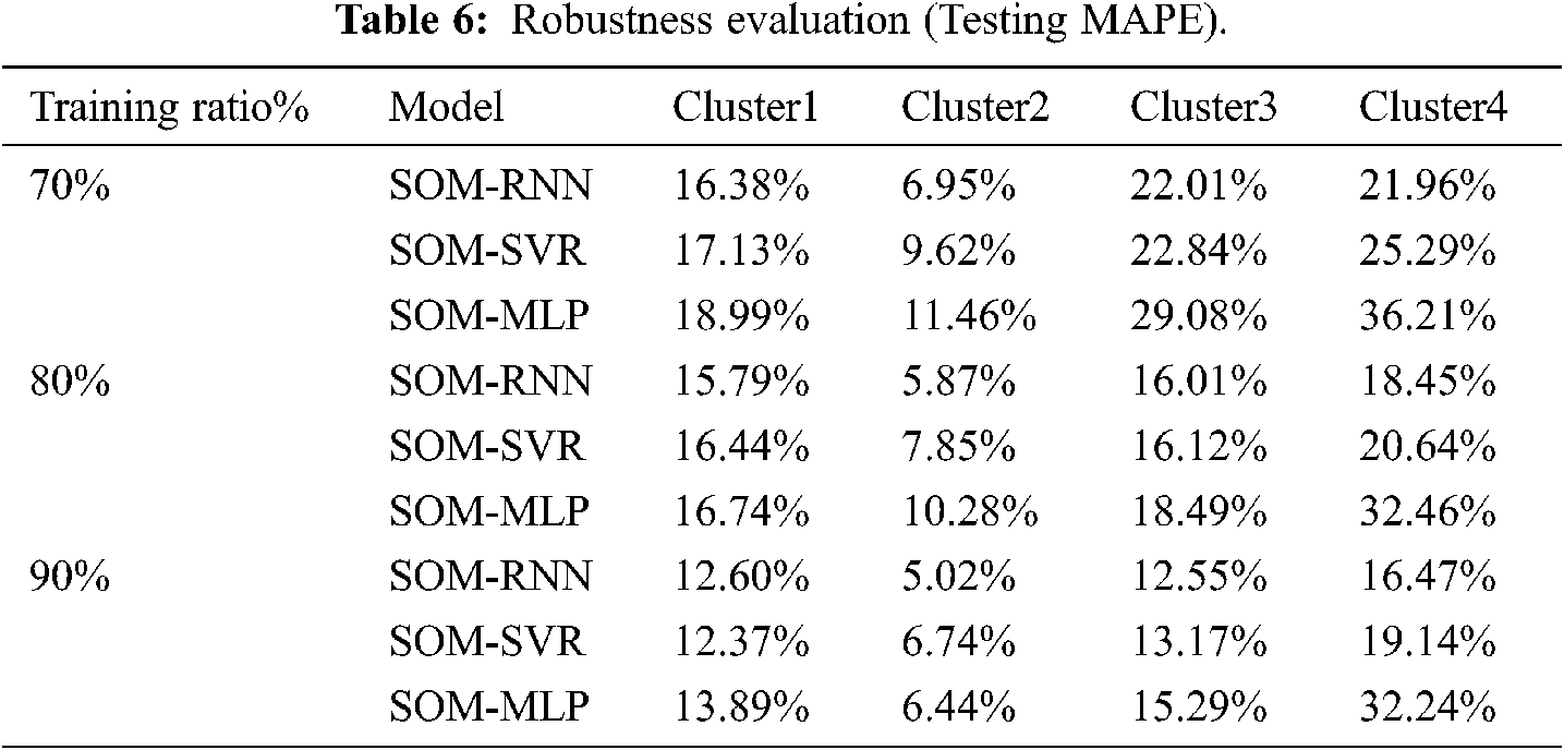
In Tab. 6, it can be observed that the proposed SOM-RNN method outperforms the other benchmarking tools under all four different ratios in terms of the four different performance measures. It therefore indicates that SOM-RNN approach indeed provides better forecast accuracy than the other two approaches.
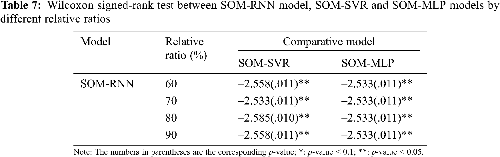
In order to test whether the proposed SOM-RNN model is superior to the comparison models in inter-purchase time prediction, the Wilcoxon signed-rank test is applied for SOM- RNN model. The Wilcoxon signed-rank test is a distribution-free, non-parametric technique which determines whether two models are different by comparing the signs and ranks of prediction values. The Wilcoxon signed-rank test is one of the most popular tests in evaluating the predictive capabilities of two different models [35–37]. For the details of the Wilcoxon signed-rank test, please refer to [35,36]. We employ the test to evaluate the predictive performance of the proposed method and the other competing models under different ratios of the size of the training data set to the completely entire average purchase behavior dataset. Tab. 7 presents the Z statistic values of the two-tailed Wilcoxon signed-rank test for RMSE values between the proposed RNN model and the other competing models in four clusters. It can be observed from Tab. 7, under different ratios, that the RMSE values of the proposed SOM-RNN model are significantly different from the comparison models. We can therefore conclude that the proposed SOM-RNN model is significantly better than the comparison models in inter-purchase time prediction.
3.6 Interpretation of Variable Importance
To help researchers understand the prediction, it is necessary to realize the importance of different features in the models. Deep learning models are difficult to interpret because of their complex structures and a significant number of parameters. To evaluate the importance of features in RNN models, we employed the permutation importance method. The permutation importance method initially proposed by Breiman [38] is an approach for ranking predictor importance and can be used for traditional machine learning models and deep learning methods. In this study, we used a python package called Eli5 [39] to execute the permutation importance method. In fact, in permutation importance, the columns of the features are shuffled, one at a time. After each shuffle, the model is re-evaluated with one incorrect feature data. Here, if the model's performance (RMSE) significantly reduces after the shuffling of a feature, that shuffled feature is deemed to have high predictive power. On the other hand, if the model performance is unaffected, then the shuffled feature is assumed to have little to no predictive power. This step is repeated for all features in the feature space. To cater for possible dependence on random variation, the permutation importance scores were calculated ten times and then averaged in this study. More details regarding permutation importance can be found in Altmann et al. [9]. The variable importance obtained for the best model in each cluster is presented in Fig. 5 (on the y-axis the increase in MSE is measured). As shown in Fig. 5, the average increase values in the MSE obtained from the permutation importance are rather small. However, instead of interpreting the raw average increase value, we focused on the average importance ranking of each feature. From Fig. 5, it was observed that, for customers in all clusters, variable X1 (Whether the tth transaction was made in weekday) is the variable which influences the prediction of inter-purchase time most. On contrary, X2 (Whether the tth transaction was made in weekend) have less impact on the prediction of inter-purchase time.

Figure 5: The variable importance obtained for the best model in each cluster
The SOM–RNN model proposed in this study not only improved the inter-purchase time prediction accuracy, discovered purchase behaviors of website customers, but also made a substantial contribution to search engine optimization (SEO) and product marketing. Relevant research results can assist website managers in determining approaches to adjust web content to shorten inter-purchase time of customers, as well as help marketing executives gain a clear understanding of adopting certain measures to shorten inter-purchase time. In addition, the inter-purchase time prediction method for website customers proposed by this study provided a systematic description and application programs for the e-commerce platforms of different industries, which can contribute to the growth and development of companies.
The result of this study also indicates that search engine design supervisors should provide suitable product information according to customer purchase behavior and product preference, indirectly inducing Google to provide more organic search traffic to reward the webpage. Moreover, marketing professionals can shorten sentences and use content chunking to ensure that product information can be digested according to the product preferences of website customers. Furthermore, keywords or visual effects can be added at appropriate times to induce customers to spend more. For example, for customers who prefer to purchase manicure products via mobile phone at midnight during weekdays, the e-retailer can provide timely information on manicure products at midnight to stimulate the desire to purchase.
This paper proposed an inter-purchase time prediction model by integrating SOM and RNN (SOM-RNN). SOM was applied to group customers according to the similarity of behavior. Then, for each cluster, customer’s purchase behavior data were applied to RNN to construct inter-purchase time prediction model. Finally the permutation importance method was employed to rank the importance of features in the inter-purchase time prediction models. The transaction data provided by a leading e-retailer in Taiwan was used to evaluate the proposed method. Moreover, this study compares the proposed method with SOM-SVR, SOM-MLP and single RNN using prediction error as criteria. The empirical results show that the suitable SOM-RNN models with variable importance interpretation can be developed, and the optimal hyper-parameter values are searched to predict inter-purchase time of customers. Moreover, the sensitivity analysis has also been performed to test the consistency of the proposed model. One of the key findings of the results is that the website purchase behavior identified by SOM in this study can be used to develop optimal search engine strategies and marketing tactics.
Funding Statement: The authors gratefully acknowledge financial support of the MOST 110-2221-E-027-110.
Conflicts of Interest: The authors declare that they have no conflicts of interest to report regarding the present study.
1. D. C. Schmittlein, D. G. Morrison and R. Colombo, “Counting your customers: Who are they and what will they do next?,” Management Science, vol. 33, no. 1, pp. 1–24, 1987. [Google Scholar]
2. G. M. Allenby, R. P. Leone and L. Jen, “A dynamic model of purchase timing with application to direct marketing,” Journal of the American Statistical Association, vol. 94, no. 446, pp. 65–374, 1999. [Google Scholar]
3. J. Chiang, C. F. Chung and E. T. Cremers, “Promotions and the pattern of grocery shopping time,” Journal of Applied Statistics, vol. 28, no. 7, pp. 801–819, 2001. [Google Scholar]
4. L. Jen, C. H. Chou and G. M. Allenby, “The importance of modeling temporal dependence of timing and quantity in direct marketing,” Journal of Marketing Research, vol. 46, no. 4, pp. 482–493, 2009. [Google Scholar]
5. P. S. Fader, B. G. S. Hardie and K. L. Lee, “Counting your customers: The easy way: An alternative to the Pareto/NBD model,” Marketing Science, vol. 24, no. 2, pp. 275–284, 2005. [Google Scholar]
6. R. Colombo and W. Jiang, “A stochastic RFM model,” Journal of Interactive Marketing, vol. 13, no. 3, pp. 2–12, 1999. [Google Scholar]
7. G. Shani, D. Heckerman and R. I. Brafman, “A MDP-based recommender system,” Journal of Machine Learning Research, vol. 6, no. 43, pp. 1265–1295, 2005. [Google Scholar]
8. M. Tavakol and U. Brefeld, “Factored MDPs for detecting topics of user sessions,” in Proc. of the 8th ACM Conf. on Recommender Systems, Foster City, CA, USA, 2014. [Google Scholar]
9. A. Altmann, L. Tolosi, O. Sander and T. Lengauer, “Permutation importance: A corrected feature importance measure,” Bioinformatics, vol. 26, no. 10, pp. 1340–1347, 2010. [Google Scholar]
10. N. K. Ahmed, A. F. Atiya, N. E. Gayar and H. El-Shishiny, “An empirical comparison of machine learning models for time series forecasting,” Econometric Reviews, vol. 29, no. 5, pp. 594–621, 2010. [Google Scholar]
11. E. Alpaydin, Machine Learning: Introduction to Machine Learning, New York: The MIT Press, 2004. [Google Scholar]
12. T. Hastie, R. Tibshirani and J. Friedman, The Elements of Statistical Learning: Data Mining, Inference, and Prediction, 2nded., New York: Springer, 2009. [Google Scholar]
13. J. Fang, X. Song, N. Yao and M. Shi, “Application of FCM algorithm combined with artificial neural network in TBM operation data,” Computer Modeling in Engineering & Sciences, vol. 126, no. 1, pp. 397–417, 2021. [Google Scholar]
14. N. Ganatra and A. Patel, “A comprehensive study of deep learning architectures, applications and tools,” International Journal of Computer Sciences and Engineering, vol. 6, no. 12, pp. 701–705, 2018. [Google Scholar]
15. T. Mikolov, M. Karafiát, L. Burget, J. Černocký and S. Khudanpur, “Recurrent neural network based language model,” in Proc. of INTERSPEECH, Makuhari, Chiba, Japan, pp. 1045–1048, 2010. [Google Scholar]
16. I. Sutskever, O. Vinyals and Q. V. Le, “Sequence to sequence learning with neural networks,” in Proc. of NIPS, Montreal, Canada, pp. 3104–3112, 2014. [Google Scholar]
17. X. Li, W. Shang and S. Wang, “Text-based crude oil price forecasting: A deep learning approach,” International Journal of Forecasting, vol. 35, no. 4, pp. 1548–1560, 2018. [Google Scholar]
18. L. Yu, Y. Zhao, L. Tang and Z. Yang, “Online big data-driven oil consumption forecasting with Google trends,” International Journal of Forecasting, vol. 35, no. 1, pp. 213–223, 2019. [Google Scholar]
19. C. Yin and J. Han, “Dynamic pricing model of e-commerce platforms based on deep reinforcement learning,” Computer Modeling in Engineering & Sciences, vol. 127, no. 1, pp. 291–307, 2021. [Google Scholar]
20. S. Xie, Z. Yu and Z. Lv, “Multi-disease prediction based on deep learning: A survey,” Computer Modeling in Engineering & Sciences, vol. 128, no. 2, pp. 489–522, 2021. [Google Scholar]
21. A. Beutel, P. Covington, S. Jain, C. Xu, J. Li et al., “Latent cross: Making use of context in recurrent recommender systems,” in Proc. of NIPS, Marina Del Rey, CA, USA, pp. 46–54, 2018. [Google Scholar]
22. T. Donkers, B. Loepp and J. Ziegler, “Sequential user-based recurrent neural network recommendations,” in Proc. of RecSys, Como, Italy, pp. 152–160, 2017. [Google Scholar]
23. B. Hidasi and D. Tikk, “General factorization framework for context-aware recommendations,” Data Mining and Knowledge Discovery, vol. 30, no. 2, pp. 342–371, 2016. [Google Scholar]
24. J. Manotumruksa, C. Macdonald and I. Ounis, “A contextual attention recurrent architecture for context-aware venue recommendation,” in Proc. of SIGIR, Ann Arbor, MI, USA, pp. 555–564, 2018. [Google Scholar]
25. M. Quadrana, A. Karatzoglou, B. Hidasi and P. Cremonesi, “Personalizing session-based recommendations with hierarchical recurrent neural networks,” in Proc. of RecSys, Como, Italy, pp. 130–137, 2017. [Google Scholar]
26. T. Kohonen, “Self-organized formation of topologically correct feature maps,” Biological Cybernetics, vol. 43, no. 1, pp. 59–69, 1982. [Google Scholar]
27. Y. LeCun, Y. Bengio and G. Hinton, “Deep learning,” Nature, vol. 521, no. 7553, pp. 436–444, 2015. [Google Scholar]
28. J. Wang and G. Wu, “Multilayer recurrent neural networks for online synthesis of asymptotic state estimators for linear dynamic-systems,” International Journal of System Science, vol. 26, no. 5, pp. 1205–1222, 1995. [Google Scholar]
29. R. E. Bucklin and C. Sismeiro, “Click here for Internet insight: Advances in clickstream data analysis in marketing,” Journal of Interactive Marketing, vol. 23, no. 1, pp. 35–48, 2009. [Google Scholar]
30. R. Olbrich and C. Holsing, “Modeling consumer purchasing behavior in social shopping communities with clickstream data,” International Journal of Electronic Commerce, vol. 16, no. 2, pp. 15–40, 2011. [Google Scholar]
31. P. J. Danaher, G. W. Mullarkey and S. Essegaier, “Factors affecting web site visit duration: A cross-domain analysis,” Journal of Marketing Research, vol. 43, no. 2, pp. 182–194, 2006. [Google Scholar]
32. W. Moe and P. S. Fader, “Capturing evolving visit behavior in clickstream data,” Journal of Interactive Marketing, vol. 18, no. 1, pp. 5–19, 2003. [Google Scholar]
33. R. E. Bucklin and C. Sismeiro, “A model of web site browsing behavior estimated on clickstream data,” Journal of Marketing Research, vol. 40, no. 3, pp. 249–267, 2003. [Google Scholar]
34. S. Kagan and R. Bekkerman, “Predicting purchase behavior of website audiences,” International Journal of Electronic Commerce, vol. 22, no. 4, pp. 510–539, 2018. [Google Scholar]
35. F. X. Diebold and R. S. Mariano, “Comparing predictive accuracy,” Journal of Business and Economic Statistics, vol. 13, no. 3, pp. 253–263, 1995. [Google Scholar]
36. A. C. Pollock, A. Macaulay, M. E. Thomson and D. Önkal, “Performance evaluation of judgmental directional exchange rate predictions,” International Journal of Forecasting, vol. 21, no. 3, pp. 473–488, 2005. [Google Scholar]
37. N. R. Swanson and H. White, “Forecasting economic time series using flexible versus fixed specification and linear versus nonlinear econometric models,” International Journal of Forecasting, vol. 13, no. 4, pp. 439–461, 1997. [Google Scholar]
38. L. Breiman, “Random forests,” Journal of Machine Learning, vol. 45, no. 1, pp. 5–32, 2001. [Google Scholar]
39. M. Korobov and K. Lopuhin, “Permutation Importance – ELI5 0.8.1 Documentation,” 2017. [Online]. Available: https://eli5.readthedocs.io/en/latest/blackbox/permutation_impo. [Google Scholar]
 | This work is licensed under a Creative Commons Attribution 4.0 International License, which permits unrestricted use, distribution, and reproduction in any medium, provided the original work is properly cited. |