DOI:10.32604/csse.2022.020869
| Computer Systems Science & Engineering DOI:10.32604/csse.2022.020869 | |
| Article |
An Approximate Numerical Methods for Mathematical and Physical Studies for Covid-19 Models
Department of Mathematics, College of Science, Taif University, Taif, 21944, Saudi Arabia
*Corresponding Author: Amr M. S. Mahdy. Email: amattaya@tu.edu.sa
Received: 12 June 2021; Accepted: 22 September 2021
Abstract: The advancement in numerical models of serious resistant illnesses is a key research territory in different fields including the nature and the study of disease transmission. One of the aims of these models is to comprehend the elements of conduction of these infections. For the new strain of Covid-19 (Coronavirus), there has been no immunization to protect individuals from the virus and to forestall its spread so far. All things being equal, control procedures related to medical services, for example, social distancing or separation, isolation, and travel limitations can be adjusted to control this pandemic. This article reveals some insights into the dynamic practices of nonlinear Coronavirus models dependent on the homotopy annoyance strategy (HPM). We summon a novel sign stream chart that is utilized to depict the Coronavirus model. Through the numerical investigations, it is uncovered that social separation of the possibly tainted people who might be conveying the infection and the healthy virus-free people can diminish or interrupt the spread of the infection. The mathematical simulation results are highly concurrent with the statistical forecasts. The free balance and dependability focus for the Coronavirus model is discussed and the presence of a consistently steady arrangement is demonstrated.
Keywords: Covid-19 model; optimal control; existence of uniformly stable; signal stream chart; homotopy perturbation technique
Over the most recent couple of years, various numerical models have been created to give smart subtleties into numerous issues of interest including the transmission and control of irresistible illnesses [1–3]. The description of the ongoing pandemic of Coronavirus, as viral pneumonia in late 2019 in Wuhan-China which has spread worldwide across 210 countries is “SARS-CoV-2” [4–6]. It is seething around the world with a tremendous cost as far as human, financial, and social effects [7–9]. Within a limited ability to focus, this brings a caution up in each country everywhere in the world like a pandemic sickness, which encourages every country to estimate the beneficiary preparatory activities to control and contain the wild spread of the infection as the seriousness of the illness will hurt human existence severely [10–12]. Since the novel Covid is new to the world to figure some effect of the pandemic circumstance and to fabricate an alleviation plan, the similitude impacts of Severe Acute Respiratory Syndrome (SARS) and (Center East Respiratory Condition) scourges in 2003 and 2009 were utilized for study and investigation [13–15]. From the investigation of the underlying spread of Coronavirus, a considerable lot of numerical models were utilized in the demonstration from benefactors across the world to decide the seriousness of the spread [16–18]. At whatever point an infectious sickness expands its feeder, it follows certain examples of spread, which broadly assist us with distinguishing and screening the elements of the illness flare-ups [19–21]. The strategy we used to appraise the spread of the sickness is a factor that drives us to finish the actions to dispose of irresistible infections [22–24]. The episode of the infection inside the country or state for time is normally nonlinear, which moves us to plan the framework where we can contemplate those dynamic nonlinear wonders [25–27]. By this framework, we can be ready to characterize the transmission of such a viral infection, which assists us to interpret the medicinal measures to stop or contain the spread of this infectious illness [28–30].
Recently, the quantity of passings throughout the planet has expanded significantly because of the spread of the new infection known as Covid-19 (Coronavirus). The quick heightening of cases in practically all nations has created a genuine test for the whole world particularly when the World Health Organization proclaimed that this infection has turned into a pandemic since its outbreak and quickly spread from China to the rest of the world. Most nations throughout the whole planet have implemented the recommended protocols to contain the development of the virus and to limit the spread of its conceivably lethal infection in all countries. Regardless of the adverse consequences on local economies and financial well-being, limiting the virus development is viewed as quite possibly the best approach to slow the infection transmission both locally and across the world. The number of infected cases globally has increased reaching 29 million so far. Consequently, the spread of Covid-19 is perceived as being quite possibly the worst disease outbreak over the last forty years. At this stage, there is no antibody against Covid-19 and most people have not yet acquired the resistance that can protect them against such a disease. As such, it is vital to address the current conditions of Covid-19 in order to forestall the disease and to take the necessary steps to contain any additional spread of its infection. In view of the reports of immunologists and clinical experts, the virus mainly spreads through respiratory droplets when an infected person coughs, sneezes, or speaks in close proximity to healthy people. Accordingly, scientists have been strongly advocating social separation between possibly contaminated people and healthy individuals to mitigate or reduce the transmission rate among local communities across countries. The test of Coronavirus is presently attracting specialists from medicine and atomic science to apply math in numerical displaying that can assume a huge part in anticipating, evaluating, and controlling the likely situations. For more extra solving the modelling mathematics [31–50].
Avoidance of Coronavirus, other than the significance of forcing general wellbeing and contamination control measures to forestall or diminish the transmission of SARS-CoV-2, the way to containing this worldwide pandemic is by inoculation to forestall SARS-CoV-2 disease in masses across the world. Exceptional endeavors in worldwide examination during this pandemic have brought about the advancement of novel immunizations against SARS-CoV-2 at a phenomenal speed to contain this viral ailment that has crushed nations worldwide and has had a descending spiraling impact on the worldwide economy.
Inoculation triggers the insusceptible framework prompting the creation of killing antibodies against SARS-CoV-2. Consequences of a progressing global, fake treatment controlled, eyewitness, dazed, urgent adequacy preliminary announced that people 16 years old or more established getting two-portion routine the preliminary immunization BNT162b2 (mRNA-based, BioNTech/Pfizer) when given 21 days separated presented 95% insurance against Coronavirus with a wellbeing profile like other viral vaccines. Results from another multicenter, Stage 3, randomized, spectator dazed, fake treatment controlled preliminary exhibited that people who were randomized to get two dosages of mRNA-1273 (mRNA based, Moderna) antibody given 28 days separated showed 94.1% viability at forestalling Coronavirus sickness, and no security concerns were noted other than mild fever and transient reactions. In light of the aftereffects of these antibody adequacy preliminaries, the FDA gave two EUAs, one on December 11, 2020, allowing the utilization of the BNT162b2 immunization, and another on December 18, 2020, conceding the utilization of the mRNA-1273 antibody for the avoidance of Coronavirus. A third immunization, Ad26.COV2.S for the avoidance of Coronavirus got EUA by the FDA on February 27, 2021, in light of a multicenter, fake treatment control, stage preliminary showed that a solitary portion of Ad26.COV2.S antibody presented 73% viability in the US in forestalling Coronavirus (information not yet distributed).
Therefore, the present study was undertaken to fill in this gap of knowledge.
Fig. 1, shows the sign stream chart
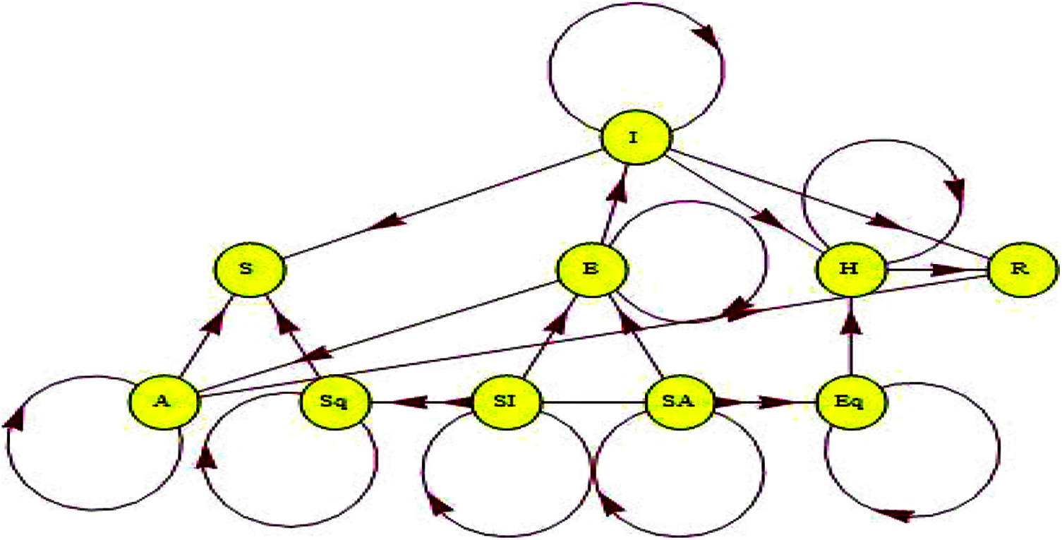
Figure 1: Suggestion signal stream chart of the model
Using a signal stream chart to act the dynamical systems is much profitable to view, for example [9,13].
A signal stream chart is a scheme agent that is used to display the interrelation among the system states and become possible to utilize scheme-theoretic stuff to find novel brow of the system.
2 Optimal Control for Covid-19 Modeling
Consider the state presented (1), in
where
Defined the functional objective is (quadratic is the control variable)
Minimizes function objective at it [28–34]:
where
The following initial conditions are satisfied:
OCP is defined, consider the a modified objective function:
where the objective function of Hamiltonian (6) as follows:
Applying Pontryagin's maximum principal, from (6) and (8), conditions necessary and sufficient OPC is
where
We construct the theorem at similar [12,13,30,31]:
Theorem 1.
If
(i) Co-state equation
(ii) With condition transversality:
(iii) Optimality conditions
So, the functions control
For a lot of optimal control and model differentials, equations for solving models see [1,29].
3 Existence of Uniformly Stable Solution
This subsection explores the existence of uniformly stable solution. Let us define
Let
This means such all of the 8 functions
4 Invariance and Symmetry of the Proposed Model
For system (1), the transformation
Then if
Also, we proved the divergence of the proposed paradigm (1) as follows
Then proposed model paradigm (1) is dissipative such as
5 HPM Approximates the Solution for Nonlinear COVID-19 Model
Here, we present the scientific approximate solution to the COVID-19 (1). By utilizing MHPM procedure [22,23], we develop a homotopy
As per the HPM method, we guess the arrangements of conditions (17) and (24) as a force arrangement in
Inserting Eqs. (25)–(32) into Eqs. (17)–(24) and setting the coefficient of p to be zero, we deduce the following system of ODE’s as follows:
With the initial conditions:
Now, we solve the over system of ordinary differential Eqs. (33)–(56) with the initial conditions (57)–(64) to get the results:
The results of the first iteration are given by:
The results of the second iteration are given by
Using computer programs, repetitions were made up to the third order, but due to the large size of the ensuing results, they were not written to relieve to the reader and the large size of the resulting equations. Then, the approximate solutions are given by
From the initial values in Wuhan, China, the parameters in the approximate solutions (68)–(74) are given by as
The approximate solutions (68)–(74) are given by:
Figs. 2–9 shows the responses of the model. Which the behavior between the related parameters and time also, shows the efficiency of the proposed style is highly amended.
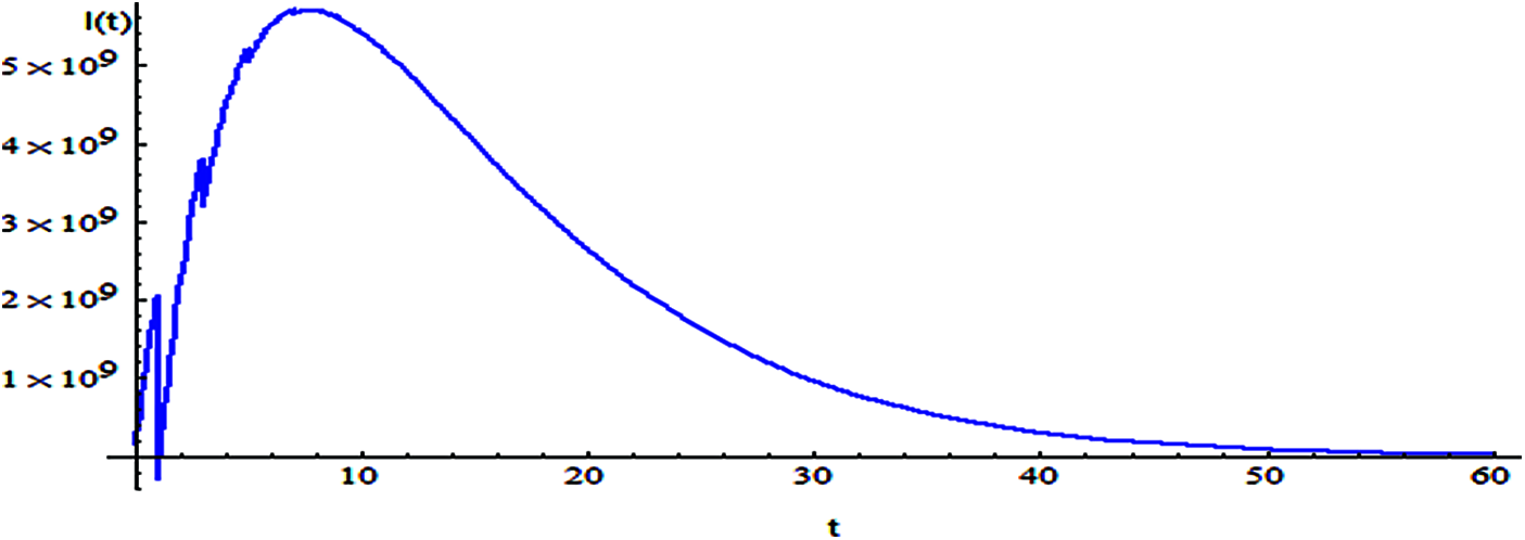
Figure 2: The relation of variable I and t
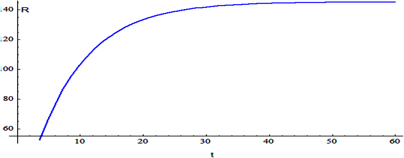
Figure 3: The relation of variable R and t
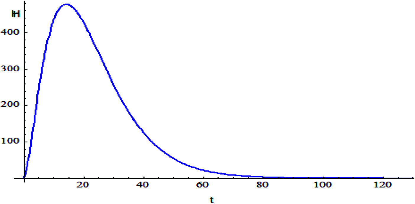
Figure 4: The relation of variable IH and t
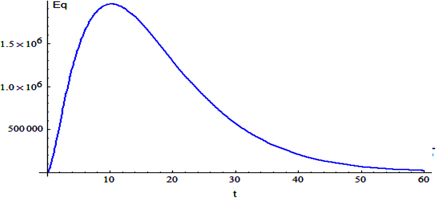
Figure 5: The relation of variable Eq and t
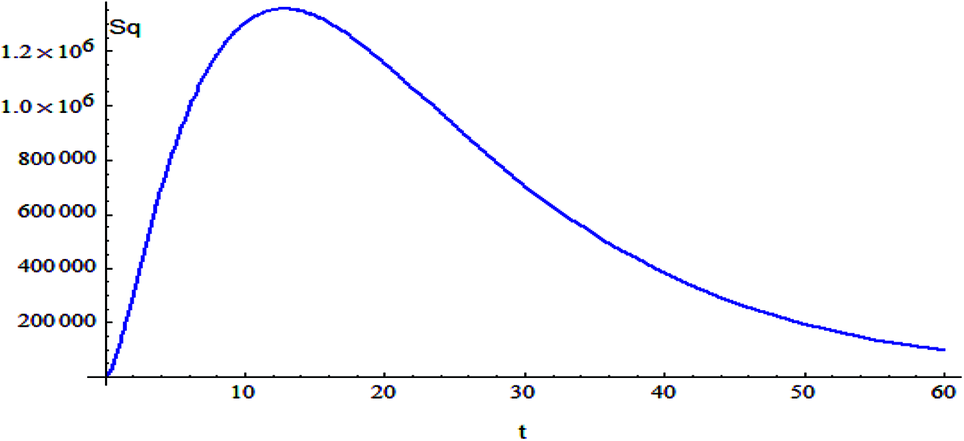
Figure 6: The relation of variable Sq and t
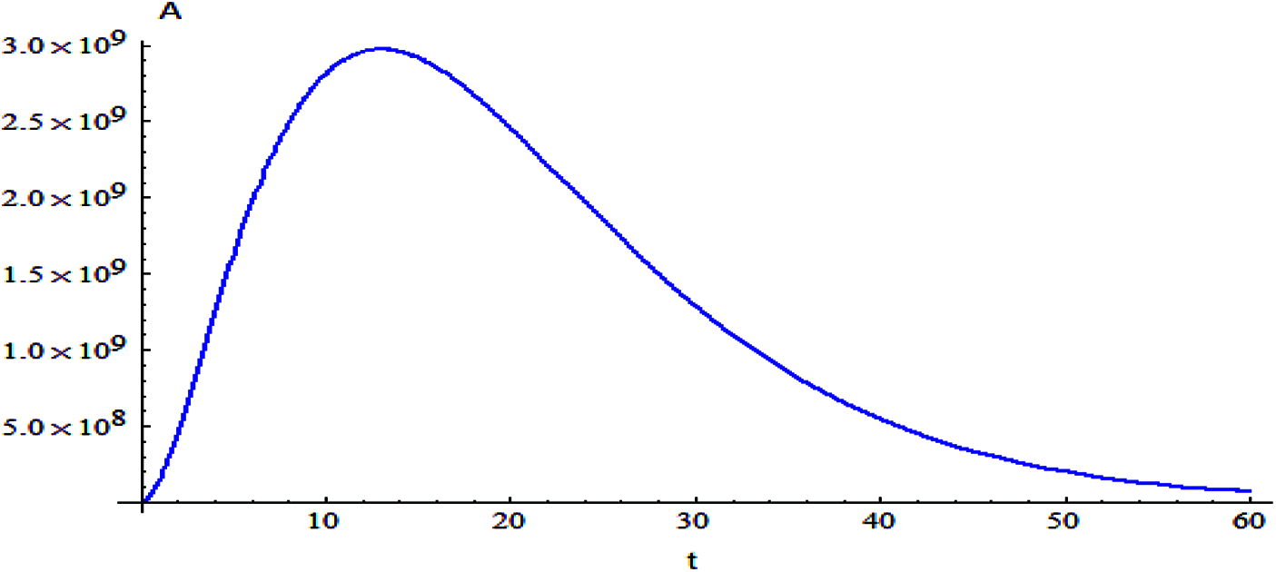
Figure 7: The relation of variable A and t
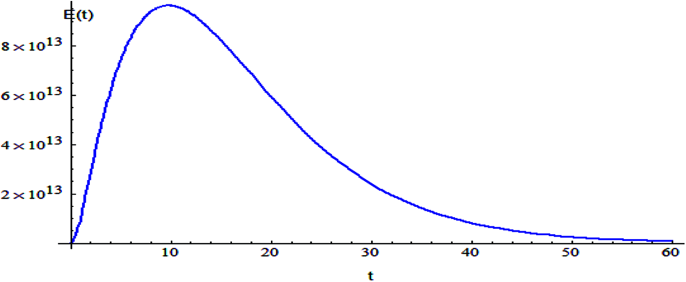
Figure 8: The relation of variable E and t
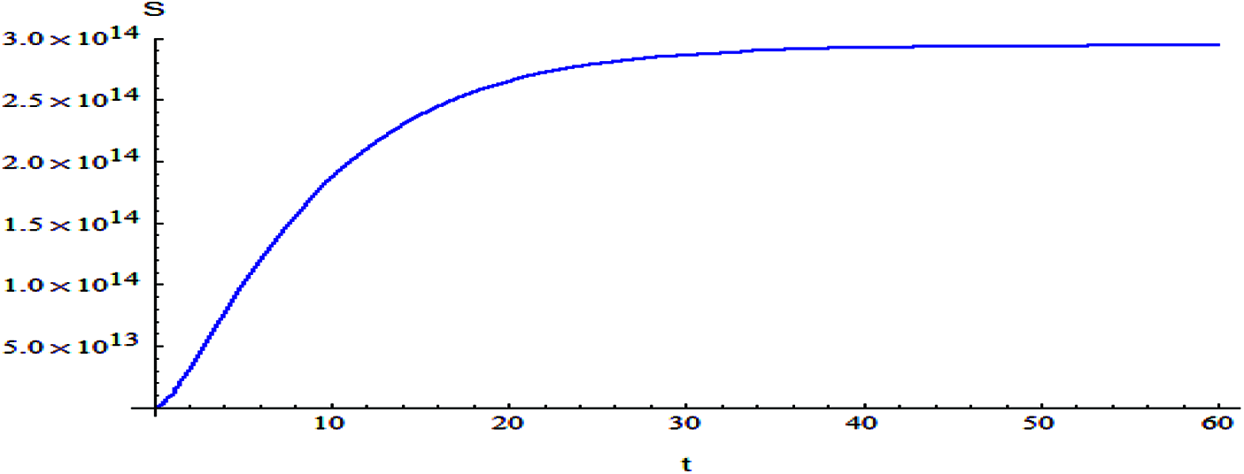
Figure 9: The relation of variable S and t
This article investigates the conduct of the Coronavirus model by utilizing the homotopy annoyance and decreased differential change techniques. The free infection balance and soundness point for the Coronavirus model are addressed. The model is portrayed by a novel sign stream graph where the signal stream chart is a scheme agent that is applied to display the interrelation among the system states and becomes possible to utilize scheme-theoretic stuff to find novel brow of the system. Through our numerical investigations, the seriousness of the infection is explained, which shows more impact by expanding the contact number. The mathematical recreations show that the nearby association among helpless and irresistible people is a significant danger factor for spreading the infection while keeping up actual distance is fundamental to decrease the danger of spreading the infection.
Acknowledgement: The authors acknowledge the support and fund provided by the Deanship of Scientific Research, Taif University, KSA [research project number 1-441-23].
Funding Statement: The authors acknowledge the support of “Taif University Deanship of Scientific Research Project number (1-441-23), Taif University, Taif, Saudi Arabia”.
Conflicts of Interest: The authors declare that they have no conflicts of interest to report regarding the present study.
1. C. I. Siettos and L. Russo, “Mathematical modeling of infectious disease dynamics,” Virulence, vol. 4, no. 4, pp. 295–306, 2013. [Google Scholar]
2. S. M. Jenness, S. M. Goodreau and M. Morris, “Epimodel: An R package for mathematical modeling of infectious disease over networks,” Journal of Statistical Software, vol. 84, no. 8, pp. 1–56, 2018. [Google Scholar]
3. O. Angulo, F. Milner and L. Sega, “A sir epidemic model structured by immunological variables,” Journal of Biological Systems, vol. 21, no. 4, pp. 1340013, 2013. [Google Scholar]
4. F. Castiglione, F. Pappalardo, C. Bianca, G. Russo and S. Motta, “Modeling biology spanning different scales: An open challenge,” BioMed Research International, vol. 2014, no. 1–4, pp. 1–9, 2014. [Google Scholar]
5. K. A. Gepreel, M. S. Mohamed, H. Alotaibi and A. M. S. Mahdy, “Dynamical behaviors of nonlinear coronavirus (covid-19) model with numerical studies,” Computers, Materials Continua, vol. 67, no. 1, pp. 675–686, 2021. [Google Scholar]
6. A. S. Shaikh, I. N. Shaikh and K. S. Nisar, “A mathematical model of covid-19 using fractional derivative: Outbreak in India with dynamics of transmission and control,” Advances in Difference Equations, vol. 373, no. 1, pp. 1–19, 2020. [Google Scholar]
7. A. S. Shaikh, V. S. Jadhav, M. G. Timol, K. S. Nisar and I. Khan, “Analysis of the covid-19 pandemic spreading in India by an epidemiological model and fractional differential operator,” Preprints (Mathematics & Computer Science), pp. 1–16, 2020. https://doi:10.20944/preprints202005.0266.v1. [Google Scholar]
8. M. Naveed, M. Rafiq, A. Raza, N. Ahmed, I. Khan et al., “Mathematical analysis of novel coronavirus (2019-ncov) delay pandemic model,” Computers, Materials & Continua, vol. 64, no. 3, pp. 1401–1414, 2020. [Google Scholar]
9. A. M. S. Mahdy and M. Higazy, “Numerical different methods for solving the nonlinear biochemical reaction model,” International Journal of Applied and Computational Mathematics, vol. 5, no. 6, pp. 1–17, 2019. [Google Scholar]
10. A. M. S. Mahdy, “Numerical studies for solving fractional integro-differential equations,” Journal of Ocean Engineering and Science, vol. 3, no. 2, pp. 127–132, 2018. [Google Scholar]
11. Y. A. Amer, A. M. S. Mahdy and E. S. M. Youssef, “Solving fractional integro-differential equations by using sumudu transform method and Hermite spectral collocation method,” Computers Materials and Continua, vol. 54, no. 2, pp. 161–180, 2018. [Google Scholar]
12. K. A. Gepreel, M. Higazy and A. M. S. Mahdy, “Optimal control, signal flow graph, and system electronic circuit realization for nonlinear Anopheles Mosquito model,” International Journal of Modern Physics C, vol. 31, no. 9, pp. 1–18, 2020. [Google Scholar]
13. A. M. S. Mahdy, H. Higazy, K. A. Gepreel and A. A. A. El-dahdouh, “Optimal control and bifurcation diagram for a model nonlinear fractional SIRC,” Alexandria Engineering Journal, vol. 59, no. 5, pp. 1–21, 2020. [Google Scholar]
14. A. M. S. Mahdy, N. Sweilam and H. Higazy, “Approximate solution for solving nonlinear fractional order smoking model,” Alexandria Engineering Journal, vol. 59, no. 2, pp. 739–752, 2020. [Google Scholar]
15. M. A. Khan and A. Atangana, “Modeling the dynamics of novel coronavirus (2019-ncov) with fractional derivative,” Alexandria Engineering Journal, vol. 59, no. 4, pp. 2379–2389, 2020. [Google Scholar]
16. J. Li and X. Zou, “Modeling spatial spread of infectious diseases with a fixed latent period in a spatially continuous domain,” Bulletin of Mathematical Biology, vol. 71, no. 8, pp. 20–48, 2009. [Google Scholar]
17. J. G. De Abajo, “Simple mathematics on covid-19 expansion,” medRxiv preprint, pp. 1–2, 2020. https://doi.org/10.1101/2020.03.17.20037663. [Google Scholar]
18. T. M. Chen, J. Rui, Q. P. Wang, Z. Y. Zhao, J. A. Cui et al., “A mathematical model for simulating the phase-based transmissibility of a novel coronavirus,” Infectious Diseases of Poverty, vol. 9, no. 1, pp. 1–8, 2020. [Google Scholar]
19. W. O. Kermack and A. G. McKendrick, “A contribution to the mathematical theory of epidemics,” Proceedings of the Royal Society of London, Series A Containing Papers of a Mathematical and Physical Character, vol. 115, no. 772, pp. 700–721, 1927. [Google Scholar]
20. H. El-Saka, “The fractional-order sis epidemic model with variable population size,” Journal of the Egyptian Mathematical Society, vol. 22, no. 1, pp. 50–54, 2014. [Google Scholar]
21. R. Balakrishnan and K. Ranganathan, A textbook of graph theory. Berlin: Springer Science & Business Media, 2012. [Google Scholar]
22. J. H. He, “Homotopy perturbation method for solving boundary value problems,” Physics Letters A, vol. 350, no. 1–2, pp. 87–88, 2006. [Google Scholar]
23. K. A. Gepreel, “The homotopy perturbation method applied to the nonlinear fractional Kolmogorov–Petrovskii–Piskunov equations,” Applied Mathematics Letters, vol. 24, no. 8, pp. 1428–1434, 2011. [Google Scholar]
24. K. A. Gepreel, A. M. S. Mahdy, M. S. Mohamed and A. Al-Amiri, “Reduced differential transform method for solving nonlinear biomathematics models,” Computers, Materials Continua, vol. 61, no. 3, pp. 979–994, 2019. [Google Scholar]
25. A. M. S. Mahdy, Kh. Lotfy, W. Hassan and A. A. El-Bary, “Analytical solution of magneto-photothermal theory during variable thermal conductivity of a semiconductor material due to pulse heat flux and volumetric heat source,” Waves in Random and Complex Media, vol. 11, no. 3, pp. 1–18, 2020. [Google Scholar]
26. A. M. S. Mahdy and E. S. M. Youssef, “Numerical solution technique for solving isoperimetric variational problems,” International Journal of Modern Physics C, vol. 32, no. 1, pp. 1–14, 2021. [Google Scholar]
27. M. I. A. Othman and A. M. S. Mahdy, “Differential transformation method and variation iteration method for Cauchy reaction-diffusion problems,” Journal of Mathematics and Computer Science, vol. 1, no. 2, pp. 61–75, 2010. [Google Scholar]
28. Y. A. Amer, A. M. S. Mahdy and H. A. R. Namoos, “Reduced differential transform method for solving fractional-order biological systems,” Journal of Engineering and Applied Sciences, vol. 13, no. 20, pp. 8489–8493, 2018. [Google Scholar]
29. M. M. Khader, N. H. Swetlam and A. M. S. Mahdy, “The chebyshev collection method for solving fractional order klein-gordon equation,” WSEAS Transactions on Mathematics, vol. 13, pp. 31–38, 2014. [Google Scholar]
30. A. M. S. Mahdy, M. S. Mohamed, Kh. Lotfy, M. Alhazmi, A. A. El-Bary et al., “Numerical solution and dynamical behaviors for solving fractional nonlinear rubella ailment disease model,” Results in Physics, vol. 24, pp. 1–10, 2021. [Google Scholar]
31. N. H. Sweilam, S. M. Al-Mekhlafi and D. Baleanu, “Optimal control for a fractional tuberculosis infection model including the impact of diabetes and resistant strains,” Journal of Advanced Research, vol. 24, pp. 125–137, 2021. [Google Scholar]
32. M. I. A. Othman and A. M. S. Mahdy, “Numerical studies for solving a free convection boundary-layer flow over a vertical plate,” Mechanics and Mechanical Engineering, vol. 22, no. 1, pp. 41–48, 2018. [Google Scholar]
33. A. M. S. Mahdy, Kh. Lotfy, M. H. Ahmed, A. El-Bary and E. A. Ismail, “Electromagnetic hall current effect and fractional heat order for micro temperature photo-excited semiconductor medium with laser pulses,” Results in Physics, vol. 17, no. 1–9, pp. 103161, 2020. [Google Scholar]
34. A. M. S. Mahdy, Kh. Lotfy, E. A. Ismail, A. El-Bary, M. Ahmed et al., “Analytical solutions of time-fractional heat order for a magneto-photothermal semiconductor medium with Thomson effects and initial stress,” Results in Physics, vol. 18, pp. 1–11, 2020. [Google Scholar]
35. I. H. Abdel-Halim Hassan, M. I. A. Othman and A. M. S. Mahdy, “Variational iteration method for solving: Twelve order boundary value problems,” International Journal of Mathematical Analysis, vol. 3, no. 13–16, pp. 719–730, 2009. [Google Scholar]
36. A. M. S. Mahdy, M. S. Mohamed, K. A. Gepreel, A. AL-Amiri and M. Higazy, “Dynamical characteristics and signal flow graph of nonlinear fractional smoking mathematical model,Chaos,” Solitons & Fractals, vol. 141, pp. 1–13, 2020. [Google Scholar]
37. A. M. S. Mahdy, “Numerical solutions for solving model time-fractional Fokker–Planck equation,” Numerical Methods for Partial Differential Equations, vol. 37, no. 2, pp. 1120–1135, 2021. [Google Scholar]
38. A. M. S. Mahdy, Kh. Lotfy, W. Hassan and A. A. El-Bary, “Analytical solution of magneto-photothermal theory during variable thermal conductivity of a semiconductor material due to pulse heat flux and volumetric heat source,” Waves in Random and Complex Media, no. 3, pp. 1–18, 2020. [Google Scholar]
39. A. M. S. Mahdy, Kh. Lotfy, A. El-Bary, H. M. Atef and M. Allan, “Influence of variable thermal conductivity on wave propagation for a ramp-type heating semiconductor magneto-rotator hydrostatic stresses medium during photo-excited,” Waves in Random and Complex Media, pp. 1–23, 2021. [Google Scholar]
40. A. M. S. Mahdy, Y. A. Amer, M. S. Mohamed and E. S. M. Youssef, “General fractional financial models of awareness with Caputo Fabrizio derivative,” Advances in Mechanical Engineering, vol. 12, no. 11, pp. 1–9, 2020. [Google Scholar]
41. N. H. Sweilam, M. M. Khader and A. M. S. Mahdy, “Numerical studies for solving fractional-order logistic equation,” International Journal of Pure and Applied Mathematics, vol. 78, no. 8, pp. 1199–1210, 2012. [Google Scholar]
42. Y. A. Amer, A. M. S. Mahdy and E. S. M. Youssef, “Solving fractional integro-differential equations by using sumudu transform method and Hermite spectral collocation method,” Computers Materials & Continua, vol. 54, no. 2, pp. 161–180, 2018. [Google Scholar]
43. A. K. Khamis, Kh. Lotfy, A. A. El-Bary, A. M. S. Mahdy and M. H. Ahmed, “Thermal-piezoelectric problem of a semiconductor medium during photo-thermal excitation,” Waves in Random and Complex Media, pp. 1–15, 2020. [Google Scholar]
44. Y. A. Amer, A. M. S. Mahdy, T. T. Shwayaa and E. S. M. Youssef, “Laplace transform method for solving nonlinear biochemical reaction model and nonlinear emden-fowler system,” Journal of Engineering and Applied Sciences, vol. 13, no. 17, pp. 7388–7394, 2018. [Google Scholar]
45. A. D. Toit, “Outbreak of a novel coronavirus,” Nature Reviews Microbiology, vol. 18, no. 3, pp. 123, 2020. [Google Scholar]
46. C. P. E. R. E. Novel, “The epidemiological characteristics of an outbreak of 2019 novel coronavirus diseases in China,” ZhonghuaLiu Xing Bing XueZaZhi, vol. 41, no. 2, pp. 145–149, 2020. [Google Scholar]
47. C. C. Lai, T. P. Shih, W. C. Ko, H. J. Tang and P. R. Hsueh, “Severe acute respiratory syndrome coronavirus 2 (SARS-CoV-2) and corona virus disease-2019: The epidemic and the challenges,” International Journal of Antimicrobial Agents, vol. 55, no. 3, pp. 1–9, 2020. [Google Scholar]
48. S. Agrebi and A. Larbi, “Use of artificial intelligence in infectious diseases,” Artificial Intelligence in Precision Health, vol. 2020, no. 8, pp. 415–438, 2020. [Google Scholar]
49. S. Lalmuanawma, J. Hussain and L. Chhakchhuak, “Applications of machine learning and artificial intelligence for COVID-19 pandemic: A review,” Chaos Solitons and Fractals, vol. 139, pp. 1–9, 2020. [Google Scholar]
50. A. M. S. Mahdy, K. A. Gepreel, Kh Lotfy and A. A. El-Bary, “A numerical method for solving the Rubella ailment disease model,” International Journal of Modern Physics C, vol. 32, no. 7, pp. 1–15, 2021. [Google Scholar]
 | This work is licensed under a Creative Commons Attribution 4.0 International License, which permits unrestricted use, distribution, and reproduction in any medium, provided the original work is properly cited. |