DOI:10.32604/csse.2022.021784
| Computer Systems Science & Engineering DOI:10.32604/csse.2022.021784 | |
| Article |
Ensemble Nonlinear Support Vector Machine Approach for Predicting Chronic Kidney Diseases
1Department of Computer Science and Engineering, Sri Shakthi Institute of Engineering and Technology, Coimbatore, 641062, India
2Department of Computer Science and Engineering, Kongu Engineering College, Perundurai, 638060, India
3School of Computing Science and Engineering, VIT Bhopal University, Bhopal, 466114, India
4Department of Computer Science and Engineering, Sri Krishna College of Engineering and Technology, Coimbatore, 641008, India
5Department of ECE, Sri Krishna College of Engineering and Technology, Coimbatore, 641008, India
6Department of Applied Cybernetics, Faculty of Science, University of Hradec Králové, 50003, Hradec Králové, Czech Republic
*Corresponding Author: S. Prakash. Email: sprakashsresearch1@gmail.com
Received: 14 July 2021; Accepted: 22 September 2021
Abstract: Urban living in large modern cities exerts considerable adverse effects on health and thus increases the risk of contracting several chronic kidney diseases (CKD). The prediction of CKDs has become a major task in urbanized countries. The primary objective of this work is to introduce and develop predictive analytics for predicting CKDs. However, prediction of huge samples is becoming increasingly difficult. Meanwhile, MapReduce provides a feasible framework for programming predictive algorithms with map and reduce functions. The relatively simple programming interface helps solve problems in the scalability and efficiency of predictive learning algorithms. In the proposed work, the iterative weighted map reduce framework is introduced for the effective management of large dataset samples. A binary classification problem is formulated using ensemble nonlinear support vector machines and random forests. Thus, instead of using the normal linear combination of kernel activations, the proposed work creates nonlinear combinations of kernel activations in prototype examples. Furthermore, different descriptors are combined in an ensemble of deep support vector machines, where the product rule is used to combine probability estimates of different classifiers. Performance is evaluated in terms of the prediction accuracy and interpretability of the model and the results.
Keywords: Chronic disease; classification; iterative weighted map reduce; machine learning methods; ensemble nonlinear support vector machines; random forests
Living in large modern cities is affecting our health in many ways [1]. Urban populations face an increased risk of developing chronic health conditions primarily due to (i) stress associated with fast-paced urban life, (ii) sedentary lifestyles because of work conditions and lack of time, (iii) air pollution, and (iv) a disproportionate number of people living in poverty [2]. In 2012, the World Health Organization reported that ambient (outdoor air) pollution is estimated to cause three million premature deaths worldwide per year; this mortality is due to exposure to small particulate matter with a size of 10 microns (PM10), which causes cardiovascular and respiratory diseases and cancers. The vast majority (about 72%) of air pollution-related premature deaths are due to ischemic heart diseases and strokes. The percentage of the world population facing the adverse health effects of urban living is increasing.
In recent years, a pattern of chronic diseases has begun to emerge in urban living [3]. The increase in chronic illnesses and the prevalence of inactive lifestyle in the Middle East have placed great pressure on healthcare providers, especially those trying to achieve a structured patient follow-up after each therapy change. The rapid development of information and communication technology has motivated researchers to develop E-health applications, which play a major role in improving healthcare services.
The diagnosis of chronic diseases is essential in the medical field because these diseases have persisted for a long time. The leading chronic ailments include diabetes, stroke, cardiovascular disease, arthritis, cancer, and hepatitis C. The early detection of chronic diseases helps in taking preventive actions. Hence, effective treatment at the initial stage is useful for most patients. Currently, the maintenance of clinical databases is a crucial task in the field of medicine. Complete patient data consisting of various features and diagnostics related to the patient's disease should be gathered with utmost care to provide quality services. The missing values and redundant data in medical databases make medical data mining cumbersome. Good data preparation and data reduction must be realized before applying data mining algorithms because these can affect the mining results. Disease prediction can be performed quickly and easily if the data are precise, consistent, and free from noise.
Classification and prediction [4,5] are data mining techniques that use training data for model development, and the resulting model is applied on testing data to obtain prediction results. Various classification algorithms have been applied on disease datasets for the diagnosis of chronic diseases, and the results have been promising. A novel classification technique that can expedite and simplify the diagnosis of chronic diseases is needed. In this age of data explosion, voluminous amounts of medical data are generated and updated daily. Healthcare data include electronic health records, which comprise clinical reports on patients, diagnostic test reports, prescription of doctors, pharmacy-related information, and information related to patients’ health insurance, and posts on social media, such as blogs and Tweets [6,7]. Hence, an efficient, parallel data processing technique that can manage and analyze huge volumes of healthcare data is necessary.
The purpose of this research is to develop a new prediction system for chronic diseases. The main goal is to explore and develop predictive analytics. Prediction is the first step toward prevention. It allows healthcare systems to target individuals who are in need and use (limited) health resources effectively. The iterative weighted map reduce (IWMR) framework was introduced in this study to handle samples of chronic diseases. A prediction model was developed using ensemble nonlinear support vector machines (ENSVMs) and random forests (RFs) and applied to perform predictions on CKD samples. Then, the results of the prediction methods were evaluated using classification metrics, such as precision, recall, specificity, accuracy, and F-measure.
The rest of the article is arranged as follows. Section 2 presents a review of recent literature, and Section 3 implements the proposed technique. Section 4 presents the result evaluation, and Section 5 provides the conclusions and possible scopes of future research.
Caruana et al. [8] developed and validated two new risk algorithms (QKidney® Scores) for estimating (a) the individual five-year risk of moderate–severe CKD and (b) the individual five-year risk of developing end-stage kidney failure in a primary care population. A prospective open cohort study was conducted using data from 368 QResearch® general practices to develop the scores. The derived separate risk equations for men and women were the calculated measures of calibration and discrimination obtained by using the two separate validation cohorts.
Jain et al. [9] critically assessed risk models to predict CKD and its progression and evaluated their suitability for clinical purposes. The majority of CKD risk models in their work showed an acceptable-to-good discriminatory performance (area under the receiver operating characteristic curve >0.70) in the derivation sample. Calibration was rarely assessed, but the overall outcome was acceptable. Only eight CKD occurrence and five CKD progression risk models were externally validated, and they displayed modest-to-acceptable discrimination. Novel biomarkers of CKD (circulatory or genetic) can considerably improve prediction but have been unclear thus far, and studies on the impact of CKD prediction models have not been conducted yet. The limitations of risk models include the lack of ethnic diversity in derivation samples and the scarcity of validation studies. The review was limited by the lack of an agreed-on system for rating prediction models and the difficulty of assessing publication bias.
Hussein et al. [10] developed an artificial neural network (ANN)-based classification model for classifying diabetic patients into two classes. To obtain improved results, the researchers used the genetic algorithm (GA) in feature selection. GA was utilized to determine the number of neurons in the single hidden layered model. Furthermore, the model was trained with the back propagation (BP) algorithm, and the GA classification accuracies were compared. The designed models were also compared with functional link ANN (FLANN) and several classification systems, such as nearest neighbor, k nearest neighbor, nearest neighbor with backward sequential selection of features, multiple feature subset 1, and multiple feature subset 2, for data classification.
Lee et al. [11] presented two case studies, where high-performance generalized additive models with pairwise interactions were applied to real healthcare problems and obtained intelligible models with state-of-the-art accuracy. Cabe et al. [12] examined classification algorithms for disease datasets and obtained promising results by developing adaptive, automated, intelligent diagnostic systems for chronic diseases. Brisimi et al. [13] presented the chronic disease diagnosis (CDD) recommender system, which was developed based on a hybrid method by using multiple classifications and unified collaborative filtering. NG et al. [14] identified the factors that affect the health-related quality of life (HRQoL) of elderly persons with chronic diseases and developed a prediction model by considering these factors in the identification of HRQoL risk groups that require intervention. McCabe [15] created a simulation test environment by using characteristic models based on physician decision strategies. For the simulated populations of patients with type 2 diabetes, he used a specific data mining technology that could predict the encounter-specific errors of omission in representative databases of simulated physician–patient encounters.
Shalabi et al. [16] focused on two leading clusters of chronic diseases, namely heart problems and diabetic issues, and developed data-driven methods to predict hospitalizations due to the specified conditions. Gopal et al. [17] built an appropriate model for comparing and refining models that were derived from diverse cohorts, patient-specific features, and statistical frameworks. The goal of the research was to develop and evaluate a predictive modeling platform that can be used to simplify and expedite the specific process for health data.
Several CKD prediction methods are discussed in this section. However, all of them are not scalable for increased dataset samples. To solve this issue, this research introduced a parallel processing framework for efficiently handling huge dataset samples for prediction.
3 Improved Parallel Processing Framework and Machine Learning Approach for Prediction
The overall aim of this study is to investigate whether patient CKD data can be automatically analyzed to predict the hospitalization duration of patients in subsequent years. The proposed framework entails five major steps: dataset collection, preprocessing, parallel processing framework, disease prediction, and result evaluation. At the first stage of this work, samples were collected from benchmark sites. At the second stage, preprocessing was performed using min–max normalization and missing data imputation through the regression method. At the third stage, the IWMR framework was introduced to handle the samples of chronic diseases. The fourth stage included the prediction problems that were considered using machine learning methods, such as ENSVM and RF. The ENSVM classifier was utilized to create nonlinear combinations of kernel activations by using samples of the prototype for the prediction system. Furthermore, different descriptors were combined into an ensemble of deep SVMs, where the product rule was used to combine the probability estimates of different classifiers. At the last stage, the results of the prediction methods were evaluated using classification metrics. The overall representation of the proposed methodology is shown in Fig. 1.
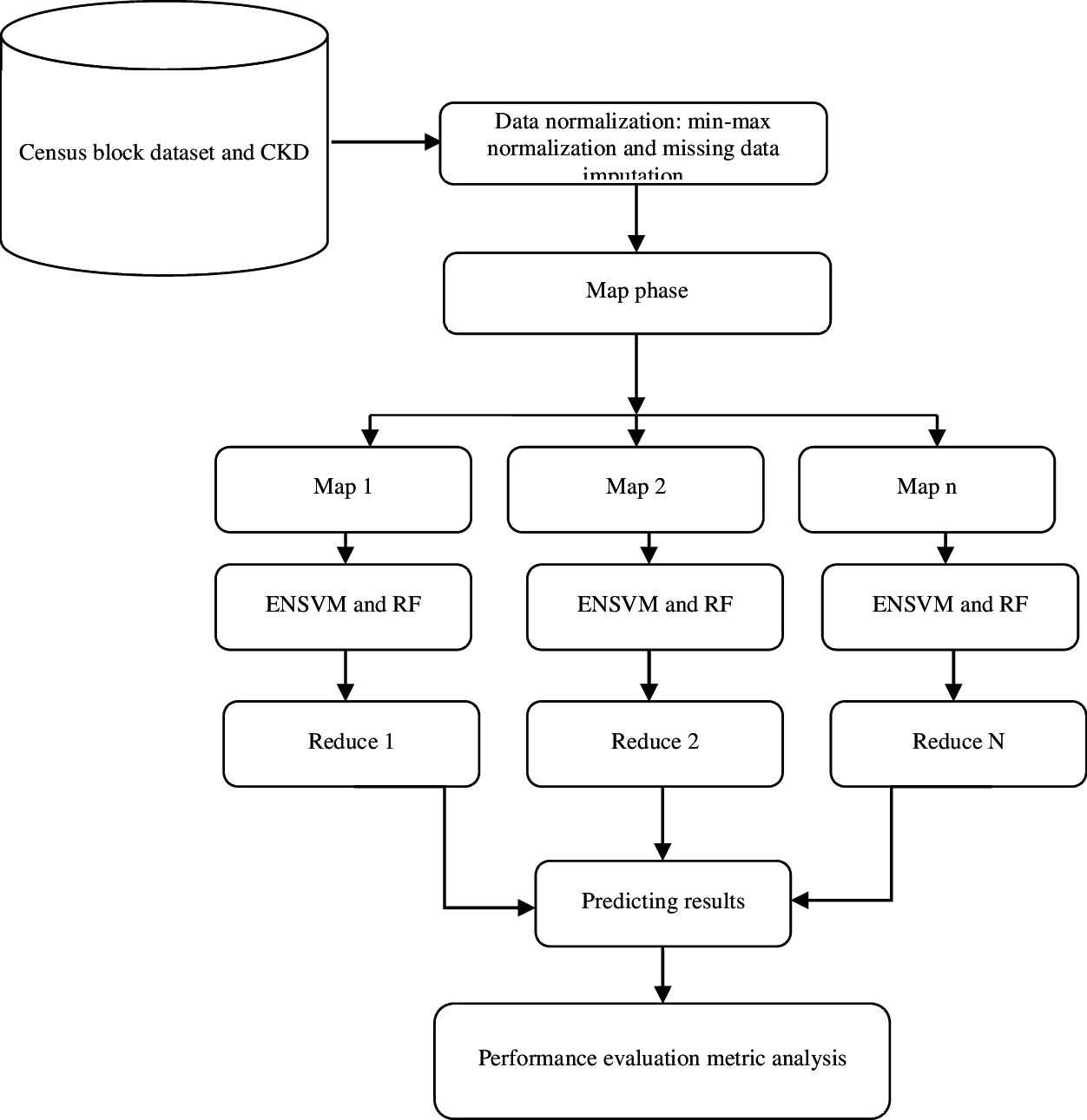
Figure 1: Proposed architecture for prediction
The census block group (CBG) is the basic granular level that the US Census Bureau reports data on, and it covers ∼1500 households. It includes all demographic data from the American Community Survey (2016), with a five-year estimation of the level of CBG. The data include the following:
• All census block group boundaries formatted as a GeoJSON file;
• Census attribute tables identified by their census table ID.
Metadata mapping provides names to a table ID, CBGs to cities and counties, and CBGs to geographic statistics, such as percentage of land and water. The census pattern files consist of the following fields: census_block_group, date_range_start, date_range_end, raw_visit_count, raw_visitor_count, visitor_home_cbgs, visitor_work_cbgs, distance_from_home, related_same_day_brand, related_same_month_brand, top_brands, popularity_by_hour, and popularity_by_day. The dataset samples were collected from https://www.kaggle.com/safegraph/census-block-group-american-community-survey-data.
The second CKD dataset was a processed version of the original from https://archive.ics.uci.edu/ml/datasets/Chronic_Kidney_Disease. The data were patient blood tests and other measures from patients with and without CKD. The dataset had 400 rows, one for each patient; these were patients seen over a period of two months before July 2015 in a hospital (Apollo Reach Karaikudi) in Tamil Nadu, India.
Of the 400 rows, 250 were related to patients with CKD, and the remaining 150 rows were for patients without CKD. This information is in the “Class” column of the dataset. Below is a description of each column from the header of the original data file with several annotations by the researcher, and each is preceded by “MB:”.
An iterative map reduce (IMR) approach based on alternating optimization was developed to handle much larger instances. We regard all vectors as column vectors. For the feature space,
3.2 Removing Patients with No Record
Before performing the normalization, patients who had no records before the target were removed because prediction could not be performed with no basis.
a.In the regression method, a regression model is fitted for each variable with missing values. On the basis of the resulting model, a new regression model is established and used to impute the missing values for the variable. Given that the data set has a motone missing data pattern, the process is repeated sequentially for variables with missing values. That is, for a variable Yj with missing values, a model
is fitted using observations with observed values for variable Yj and its covariates X1, X2, …, Xk. The following steps are implemented to generate imputed values for each imputation.
c.New parameters β∗ = (β∗0, β∗1, …, β∗(k)) and …
where g is a
where
An attribute is normalized by scaling its values so that they fall within a small specified range, such as 0.0–1.0. Min–max normalization performs linear transformation on the original data. Assume that mina and maxa are the minimum and maximum values for attribute A. Min–max normalization maps a value v of A to v’ in the range
After normalization is performed, the data are split into training and test sets randomly. Similar to supervised machine learning, the population is randomly split into training and test sets. Given that all the data points (patients’ features) are drawn from the same distribution from a statistical point of view, no differentiation is carried out between patients whose records appear earlier in time than others with later time stamps. A retrospective/prospective approach is more common in medical literature and more relevant for clinical trial settings compared with an algorithmic approach.
MapReduce [21] is the most prominent platform for big data analysis and prediction. Several previous studies have extended the MapReduce framework to achieve efficient iterative computation [22,23]. However, preliminary results show that starting a new iterative computation from scratch is extremely expensive. McSherry [24] proposed incremental iterative computations based on differential data flow, which is a new computation model that is drastically different from the MapReduce programming model. To the best of our knowledge, for the most popular platform, MapReduce, no solution has been demonstrated to efficiently handle dynamic CKD and CBG data changes for complex iterative computations. To solve this problem, an initially iterative algorithm typically performs the same computation on CKD and CBG in each iteration, thereby generating a sequence of improving results. The computation of iteration can be represented by update function F as follows:
where ND is the normalized CKD and CBG data set and R is the result set being computed. After initializing R with certain R0, the iterative algorithm computes an improved Rk from Rk−1 and ND in the k-th iteration. This process continues until it converges to a fixed point
MapReduce: A user has to submit a series of MapReduce data for an iterative algorithm. An iteration often requires at least one piece of MapReduce data. The map function processes the state CKD and CBG data, Rk−1, and the structure CKD and CBG data, ND, whereas the reduce function combines the intermediate CKD and CBG data to produce the updated state CKD and CBG data Rk. Rk is stored in the underlying distributed file system to be used as the input to the next step that implements the next iteration. The structure CKD and CBG in the iterative computation often change over time. Suppose that ND becomes
In many cases, |ΔND| ≪ |ND|, i.e., the structure CKD and CBG are changed slightly. In addition, converged fixed point
Weighted MapReduce Graph (WMRG): To implement the internal loop in MapReduce, the outputs of the reducers are sent back to the correlated mappers with their weight values. The model of this behavior is shown in Fig. 2 as WMRG. A mapper operates on state CKD and CBG record Rk (i) and structure data samples ND(i). A reducer operates on the intermediate samples and produces the updated state data samples Rk+1 (i), which are sent back to the correlated mappers or replicated to several mappers for the next iteration. WMRG has two types of vertices, namely, mapper and reducer vertices. The edges from mappers to reducers (MRE) represent the shuffled intermediate samples, and the edges from reducers to mappers (RME) represent the iterated state samples. The iterative computation continues to refine the WMRG state iteratively, including the MRE and RME states. When the MR iterative algorithm converges, the WMRG state becomes stable.

Figure 2: Weighted map reduce graph framework. (a) Iterative processing (b) Incremental processing
Incremental Iterative Processing on WMRG: Starting from the previously converged state disease, data
This idea aims to reduce unnecessary computations as much as possible. In addition, when the dataset samples increase, the identification of the correct map, a task that is given to the reduce function, becomes difficult. To solve this problem, additional weight We = (We1, …Wen) is introduced to each map function that correctly finds the exact map function. This approach reduces the computation time for searching the map function and easily iterates the process continuously. The weight values are randomly generated based on the input samples.
A map function is applied only when its input normalized disease datasets are different from those in the past iteration. A reduce function is implemented only when the state of an incoming MRE changes. The challenge is to efficiently preserve and utilize the WMRG state to realize this idea while minimizing modifications to the MR framework in order to reduce users’ programming effort.
To build the loop in WMRG, iterative MR makes map/reduce tasks persistent throughout the duration of the iterative computation. The proposed WMRG framework sends the reduce tasks’ output back to the correlated map tasks. When a map/reduce task consumes all of its currently assigned patient normalized data, it goes into an idle waiting state until it is wakened up to process new normalized data in subsequent iterations. In this manner, the constructed WMRG can perform iterative computation even in a single MapReduce job. Moreover, the input normalized data of a map function are a key-value pair of ⟨MK, MR⟩. For iterative computation, MR contains the resultant and structure normalized data. However, the two types of data have different characteristics. The proposed system distinguishes them by splitting the value argument into two. Then, a map function takes MK, WK, MRSt, MRDy where Dy is the dynamic state value and St is the structure value for the key MK and the weight value WK. Users are required to implement the new map interface.
To support the incremental processing, the converged WMRG framework state, including RME and MRE, is preserved. The RME state is the final reduce output, which is sent back and recorded in the correlated map tasks. The patient records MK, WK, MRDy, where MRDy denotes the converged dynamic state data and MK is the mapper key. MRE state is the intermediate result that is communicated from map tasks to reduce tasks and recorded in the reduced tasks. The intermediate results have the key-value pair of ⟨IK, WK, IRDy⟩, where IK is the group-by key and determines the destination reducer. Hadoop stores the intermediate results by using an IFile format. In addition, MRE state requires the source mapper. Therefore, the reducer extends the Hadoop IFile format to record ⟨MK, WK, MRSt, MRDy⟩, where MK is the source mapper key.
In this study, learning classification issues were considered for the large dataset samples. Given a training dataset
each instance NDi is a point in the d-dimensional real space ℝd and comes with a class label yi ∈ Y. We construct a decision function h: ℝd → Y in an inductive manner based on the given dataset S. The instances of NDi, h (NDi) should be equal to or very close to yi ∈ Y. Thus, the prediction of the class label of new samples NDi does not appear in the given training dataset S with h (NDi), the samples of NDi. For the classification of the large dataset, label set Y is a finite set; for example, Y = {1, 2,…, c}. In particular, Y = {−1, + 1} is a binary classification problem.
The binary classification algorithm, i.e., smooth SVM (SSVM), is used for the generation of local experts [7]. SSVM solves an unconstrained minimization problem whose formulation is given as
with a smooth p-function
In a large-scale SVM, the full kernel matrix is large and dense; hence, the full kernel matrix may not be appropriate for dealing with Eq. (10). The reduced kernel technique is used to avoid such a large and dense full kernel matrix. The key idea of the reduced kernel technique is to randomly select a small portion of data, generate a thin rectangular kernel matrix, and use this much smaller rectangular kernel matrix to replace the full kernel matrix. The formulation of reduced SSVM is expressed as follows:
where
Ensemble learning is a method that combines multiple classifiers rather than using a single classifier to obtain improved predictive performance. Ensemble learning is a reliable method that uses multiple weak learners to generate a single strong learner. In theory, even if each weak learner exhibits poor performance, ensemble learning can still generate a useful model from the ensemble of weak learners. The ENSVM algorithm is provided to apply the nonlinear method to the super-large-scale problem. The entire problem is partitioned into small ones instead of rewriting the SVM formula into a parallel algorithm. Each small set is trained by an individual nonlinear SVM. After training nonlinear SVMs, an ensemble structure that treats every nonlinear SVM as a local expert is introduced. These local experts combine their estimations to solve the entire problem. Fig. 3 shows the entire structure of the ENSVM algorithm. In this work, binary classification was the focus to simplify the problem.
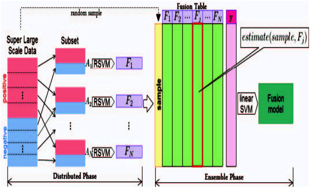
Figure 3: Ensemble nonlinear support vector machine (ENSVM) structure
The distribution phase is the first step of training. In this phase, a super-large-scale dataset is divided into many small subsets. Each subset is trained independently by an SVM to generate its own model. The next step is the ensemble phase. The term estimate (ND, FS) is used as a feature generation function, which will be defined later for combining the results of the distribution phase. The entire structure can make a nonlinear SVM for training a super-large-scale problem. Every small nonlinear SVM is independent so that it can build a nonlinear SVM model on many different machines. Additionally, a parallel processing technique is utilized in the implementation of the classifier algorithm. It has a speed advantage because the ESVM method generates nonlinear models by using small kernels rather than a single gigantic full kernel. Each trained RSVM model has a decision function of the form
A contains the instances that have the estimation of values from expert FS. wFS and bFS represent the weights and bias of the SVM model, respectively, and K is the kernel function.
Bagging (or bootstrap aggregating) is a technique for reducing the variance of an estimated predictor by averaging many noisy tools but approximately unbiased models. An RF is an ensemble of de-correlated trees. Each decision tree is formed using a training set obtained by sampling (with replacement) a random subset of the original data. While growing each decision tree, RFs use a random subset of the set of features (variables) at each node split. Essentially, the algorithm uses bagging for trees and features. Each tree is fully grown until a minimum size is reached (i.e., no pruning occurs). While the predictions of a single tree are highly sensitive to noise in its training set, the average of many trees is not, as long as the trees are not correlated. Bagging de-correlates the trees by constructing them using different training sets. To make a prediction in a new sample, RFs take the majority vote among the outputs of the grown trees in the ensemble.
The obtained data were used to evaluate various methods taken from https://www.kaggle.Com/safegraph/census-block-group-american-community-survey-data. The CKD dataset was a processed version of the original from https://archive.ics.uci.edu/ml/datasets/Chronic_Kidney_Disease. The classification performance of the classifiers was analyzed with respect to standard performance parameters, such as accuracy, specificity, sensitivity, precision, and F-measure, aside from time consumed for training (learning).
The results of four classifiers, namely, RF, linear SVM, joint clustering and classification (JCC), and ENSVM, were compared, and the results are depicted in Tabs. 1 and 2. The results of the existing and proposed methods were measured in terms of accuracy, specificity, sensitivity, precision, and F-measure.


Fig. 4 shows the performance comparison results on precision for census block and CKD datasets. Fig. 4a shows the performance comparison results on precision for census block. The proposed ESVM method showed high precision of 91.35%, whereas RF, linear SVM, and JCC produced 80.35%, 83.65%, and 87.6% precision, respectively.

Figure 4: Comparison of precision results. (a) Census block (b) Chronic kidney disease
Fig. 5 shows the performance comparison results on recall for census block and CKD datasets. Fig. 5a shows the performance comparison results on recall for census block. The proposed ESVM method had high recall of 92.15%, whereas RF, linear SVM, and JCC had 81.38%, 84.21%, and 88.32% recall, respectively.

Figure 5: Comparison of recall results. (a) Census block (b) Chronic kidney diseases
Fig. 6 shows the performance comparison results on specificity for census block and CKD datasets. Fig. 6a shows the performance comparison results on specificity for census block. The proposed ESVM method had high specificity of 89.67%, whereas RF, linear SVM, and JCC had 80.89%, 83.56%, and 86.34% specificity, respectively.

Figure 6: Comparison of specificity results. (a) Census block (b) Chronic kidney diseases
Fig. 7 shows the performance comparison results on F-measure for census block and CKD datasets. Fig. 7a shows the performance comparison results on F-measure for census block. The proposed ESVM method had a high F-measure value of 90.23%, whereas RF, linear SVM, and JCC had F-measure values of 83.25%, 86.54%, and 88.11%, respectively.

Figure 7: Comparison of F-measure results. (a) Census block (b) Chronic kidney diseases
Fig. 8 shows the performance comparison results on accuracy for census block and CKD datasets. Fig. 8a shows the performance comparison results on accuracy for census block. The proposed ESVM method had high accuracy of 93.59%, whereas RF, linear SVM, and JCC had accuracies of 84.62%, 87.19%, and 90.24%, respectively.

Figure 8: Comparison of accuracy results. (a) Census block (b) Chronic kidney diseases
The IWMR framework was introduced for the effective management of large dataset samples. The absence of records and the missing values in the data of patients with CKD were corrected using the regression method. Normalization was performed using min-max normalization, and classification methods were developed to predict hospitalizations. Moreover, a binary classification problem was formulated for prediction and solved using ENSVM and RF. The proposed work adopted a diverse set of methods, namely, ENSVM and RF. Its performance was evaluated in terms of classification accuracy and interpretability, which is an equally crucial criterion in the medical domain. In the future, the proposed work can be applied to the current system and related disease samples. Feature selection can also be examined further.
Funding Statement: The authors received no specific funding for this study.
Conflicts of Interest: The authors declare that they have no conflicts of interest to report regarding the present study.
1. G. Stahl, “Health impacts of living in a city,” Global Citizen, 2015. [Online]. Available: https://www.globalcitizen.org/en/content/health-impacts-of-living-in-a-city/. [Google Scholar]
2. D. Yach, C. Hawkes, C. L. Gould and K. J. Hofman, “The global burden of chronic diseases: Overcoming impediments to prevention and control,” Jama, vol. 291, no. 21, pp. 2616–2622, 2004. [Google Scholar]
3. J. A. Alawatia and J. Tuomilehto, “Diabetes risk score in Oman: A tool to identify prevalent type 2 diabetes among arabs of the Middle East,” Journal of Diabetes and Clinical Practice, vol. 77, pp. 438–444, 2007. [Google Scholar]
4. T. Eswari, P. Sampath and S. Lavanya, “Predictive methodology for diabetic data analysis in big data,” Proc. Comput Science, vol. 50, pp. 203–208, 2015. [Google Scholar]
5. H. Cox and C. Coupl, “Predicting the risk of chronic kidney disease in men and women in england and wales: Prospective derivation and external validation of the QKidney scores,” BMC Family Practice, vol. 11, no. 1, pp. 1–23, 2010. [Google Scholar]
6. E. Tcheugui and A. P. Kengne, “Risk models to predict chronic kidney disease and its progression: A systematic review,” PLOS Medicine, vol. 9, no. 11, 2012. [Google Scholar]
7. M. Pradhan and R. K. Sahu, “Predict the onset of diabetes disease using artificial neural network (ANN),” International Journal of Computer Science & Emerging Technologies, vol. 2, no. 2, pp. 2044–20054, 2011. [Google Scholar]
8. R. Caruana, Y. Lou, J. Gehrke, P. Koch, M. Sturm et al., “Intelligible models for healthcare: predicting pneumonia risk and hospital 30-day readmission,” in Proc. ICKDDM, Singapore, pp. 1721–1730, 2015. [Google Scholar]
9. D. Jain and V. Singh, “Feature selection and classification systems for chronic disease prediction: A review,” Egyptian Informatics Journal, vol. 19, no.3, pp. 179–189, 2018. [Google Scholar]
10. A. S. Hussein, W. M. Omar, X. Li and M. Ati, “Efficient chronic disease diagnosis prediction and recommendation system,” in Proc. IECBES, Langkawi, Malaysia, pp. 209–214, 2012. [Google Scholar]
11. S. K. Lee, Y. J. Son, J. Kim, H. G. Kim, J. I. Lee et al., “Prediction model for health-related quality of life of elderly with chronic diseases using machine learning techniques,” Healthcare Informatics Research, vol. 20, no. 2, pp. 125–134, 2014. [Google Scholar]
12. R. M. Cabe, G. Adomavicius, P. E. Johnson, G. Ramsey, G. Rund et al., “Using data mining to predict errors in chronic disease care,” Advances in Patient Safety: New Directions and Alternative Approaches, vol. 3, 2008. [Google Scholar]
13. T. S. Brisimi, T. Xu, T. Wang, W. Dai, W. G. Adams et al., “Predicting chronic disease hospitalizations from electronic health records: An interpretable classification approach,” IEEE Access, vol. 106, no. 4, pp. 690–707, 2018. [Google Scholar]
14. K. NG, A. Ghoting, S. R. Steinhubl, W. F. Stewart, B. Malin et al., “A parallel predictive modeling platform for healthcare analytic research using electronic health records,” Journal of Biomedical Informatics, vol. 48, pp. 160–170, 2014. [Google Scholar]
15. S. Gnanapriya, R. Suganya, G. S. Devi and M. S. Kumar, “Data mining concepts and techniques,” Data Mining and Knowledge Engineering, vol. 2, no. 9, pp. 256–263, 2010. [Google Scholar]
16. A. Shalabi, L. Shaaban and B. Kasasbeh, “Data mining: A preprocessing engine,” Journal of Computer Science, vol. 2, no. 9, pp. 735–739, 2006. [Google Scholar]
17. S. Gopal Krishna Patro and K. Kumar Sahu, “Normalization: A preprocessing stage,” arXiv Preprint arXiv, pp. 1–4, 2015. [Google Scholar]
18. J. Dean and S. Ghemawat, “Mapreduce: Simplified data processing on large clusters,” in Proc. Communications of the ACM, United States, vol. 4, 2004. [Google Scholar]
19. Y. Bu, B. Howe, M. Balazinska and M. D. Ernst, “Haloop: Efficient iterative data processing on large clusters,” PVLDB, vol. 3, pp. 285–296, 2010. [Google Scholar]
20. J. E. Kanayake, H. Li, B. Zhang, T. Gunarathne, S. H. Bae et al., “Twister: A runtime for iterative mapreduce,” in Proc. ICCC, New York, United States, vol. 10, 2010. [Google Scholar]
21. F. McSherry, D. G. Murray, R. Isaacs and M. Isard, “Differential dataflow,” in Proc. CIDR, USA, vol. 13, 2013. [Google Scholar]
22. Y. J. Lee and O. L. Mangasarian, “SSVM: A smooth support vector machine for classification,” Computational Optimization and Applications, vol. 20, no. 1, pp. 5–22, 2001. [Google Scholar]
23. C. J. Burges, “A tutorial on support vector machines for pattern recognition,” Data Mining and Knowledge Discovery, vol. 2, no. 2, pp. 121–167, 1998. [Google Scholar]
24. A. Mammone, M. Turchi and N. Cristianini, “Support vector machines,” Computational Statistics, vol. 1, no. 3, pp. 283–289, 2009. [Google Scholar]
 | This work is licensed under a Creative Commons Attribution 4.0 International License, which permits unrestricted use, distribution, and reproduction in any medium, provided the original work is properly cited. |