DOI:10.32604/csse.2022.022621
| Computer Systems Science & Engineering DOI:10.32604/csse.2022.022621 | |
| Article |
Multi-Objective Modified Particle Swarm Optimization for Test Suite Reduction (MOMPSO)
1Department of Information Technology, B.S.Abdur Rahman Crescent Institute of Science and Technology, Chennai, 600048, India
2Department of Computer Science and Engineering, B.S.Abdur Rahman Crescent Institute of Science and Technology, Chennai, 600048, India
*Corresponding Author: U. Geetha. Email: geetha_it_phd_17@crescent.education
Received: 13 August 2021; Accepted: 24 September 2021
Abstract: Software testing plays a pivotal role in entire software development lifecycle. It provides researchers with extensive opportunities to develop novel methods for the optimized and cost-effective test suite Although implementation of such a cost-effective test suite with regression testing is being under exploration still it contains lot of challenges and flaws while incorporating with any of the new regression testing algorithm due to irrelevant test cases in the test suite which are not required. These kinds of irrelevant test cases might create certain challenges such as code-coverage in the test suite, fault-tolerance, defects due to uncovered-statements and overall-performance at the time of execution. With this objective, the proposed a new Modified Particle Swarm optimization used for multi-objective test suite optimization. The experiment results involving six subject programs show that MOMPSO method can outer perform with respect to both reduction rate (90.78% to 100%) and failure detection rate (44.56% to 55.01%). Results proved MOMPSO outperformed the other stated algorithms.
Keywords: Regression testing; test suite reduction; test case generation
Software testing in Software Industry must be conducted thoroughly and should be kept continuous. Some challenges do arise due to the frequency with which software testing is performed in conjunction to software development. With every development it is must to perform one round of testing including sanity testing but sometimes this pattern does not get followed due to some reason like either the resource availability is not spontaneous or often executing all the test cases is quite time-consuming process [1–4]. Thus, it is being devised that some test case reduction applications can be explored for enhancement of the overall process of software testing.
Regression Testing makes use of the redundant way of testing the entire test suite but re-testing of the entire test suite is quite advantageous as it helps in making the overall test suite incorporate with some modified test cases also which is considered a good practice as it helps in identifying and predict the upcoming errors or endangered behaviors that might exist within the test-suite [5–7]. Some optimization strategies are required to introduce for solving the amplification of number of test cases with evolution of system software simultaneously [5,8–10]. Therefore, many optimization techniques are proposed in order to reduce the efforts put for regression testing by selecting few test cases from the existing test-suite [1,4,11–14]. Test case selection is one of the major roles in regression testing. With the selected test cases, the testing team will spend less time for identifying the problem. In this research we focused MOPSO Algorithm for test suite reduction in which we have used effective parameters for selecting the test cases in order to improve cost of selection process [15–18] .When any meta-heuristic related model is used for test case reduction technique then two very prime principles which must be used in contradiction whenever needed where first principle says that exploration of the space of search is very important and another principle emphasizes on exploiting the optimal solutions [3,6,7].
Another important parameter which plays a very significant role in regression testing is statement coverage which ensures that the majority of the paths of the given test case execution is performed based on traditional approach which involves some more factors like coverage information including statement [19–21], DU pair [22], branch etc. [23–25].But still some problem persists in the algorithm like for large systems the coverage of path is a tedious task as it is more time-consuming with respect to parameter of statement coverage or coverage information within the source code [13,16]. The main problem of the usage of this algorithm is its complexity in terms of computation which can be achieved when cyclomatic complexity is less than 10.
In order to satisfy the first principle related to search of space can be improvised more by balancing the exploration and exploitation feature efficiently. In this research, two different search space created to achieve multi objective optimization that includes cost, history, frequency, fault detection rate, coverage etc. Further if the need is to improvise the overall balance by following approach where two or more search space can get combined easily. Two different search spaces create the motivation to adopt the binary version of MOMPSO that really helps in reducing test cases by selecting more efficient and relevant set of test cases. Thus, the real motivation comes from the mentioned context of efficient test case reduction process and improvised test cases in the entire test suite that MOMPSO can be accepted as a revised and extracted test case suite for investigation and research. Hence main research emphasis and objectives of this paper were as follows:
• Comparison of performance is performed on the basis of certain parameters such as execution of test cases, presence of test-cases in the test bed, time consumed to perform the execution of test cases and time consumed to execute test cases against traditional approach of testing.
• To explore more of MOMPSO h algorithm which is never being researched and investigated in any of the earlier literature review surveys for test case reduction techniques in order to identify some selected set of test cases in the entire test suite.
• A brief comparison and investigation need to be performed once the MOMPSO algorithm is applied to ten different benchmark programs and then compared with other hybrid algorithms like genetic algorithm, normal PSO and normal GWO (BGWO) [19,20].
Structuring of rest of the paper is performed in the following manner where Section 2 elucidates information for optimization and information for test case reduction problem. Section 3 provides an overview about proposed algorithm. Section 4 illustrates and describes for application of proposed MOMPSO algorithm for test case reduction. Section 5 demonstrates the activity performed on the existing results with some inferences regarding the empirical evaluation.
Anu et al. has surveyed different angles related to TSR problem and they selected more than 70 papers and categorized into different area includes defect estimation method test input reduction, test automation test, test strategy and quality after and before which based on different strategy to optimizing test suite [2–5].
PSO, GA, GWO and APSO are the other four algorithms which are used for automatic generation of test cases that are basically distance based fitness function used for covering the path and test case generation [5,13,18,22,23]. Out of PSO and APSO, after the study and research ASPO is considered more profound and effective for any searching mechanism related to software testing [6,8]. But again, it is not used for test case reduction and test case execution rather it is used for enhancing TSR capabilities as depicted earlier. ACO algorithm is considered one of the most wanted and effective algorithms because of its feature of easy selection, prioritization and generation of test cases [7,8]. The most promising feature because of which it is selected for optimization technique is its ability to perform the entire software coverage without possessing any redundant set of test cases. Somewhat similar software optimization algorithms like swarm-based optimization are adopted more and more as this swarm fused algorithms can be used to generate efficient automated test environment with other software for applying and used as reduction techniques [9,10,14,15]. PSO algorithm was first developed by James Kennedy and Russell in 1995.basic idea of algorithm gathered from two main concepts one is observation of animal habits such as bird and fish and second one is the field of evolutional computation such as a genetic algorithm. It maintains multiple potential solution of one time [7,11,12,17]. In every iteration of the algorithm, an object function evaluates each solution to determine its fitness and a particle is used to represent a solution in the fitness landscape. The position of particle is updated in the search space by
Basically, two variation of PSO algorithm, one is global best and local best that have developed based on size of the neighborhoods [13,26–28]. In global best PSO, considering minimization problem, then the personal best in each iteration is calculated as
The global best position
The velocity of particle i is calculated as
In local best PSO, the velocity of particle i is calculated as
There is some parameter which are required to improve performance [26–28]. The basic parameters are no of particle, stopping criteria, velocity and coefficients factor. The term
• When c1 = c2 = 0 (all particles flying at their current speed until boundary in search space), the velocity is determined by
• When c1>0 and c2 = 0 (all particles are independent), the velocity is determined by
• When c2>0 and c2 = 0 (all attached to a single point), the velocity become
The particle fly or swarm through the search space to find the maximum value returned by the objective function and each particle maintains position in the search space, velocity and its individual best position, [11,12,17].
Swarm Intelligence (SI) algorithm is considered one of the novel algorithms which is used for performance improvement by allowing PSO in TSR for solving the multi-objective issue [5,14,19]. Also, PSO prioritization helps in improving the test cases execution time by considering selected set of test cases and eliminating the irrelevant set of test cases in turn helping by improving the code coverage information as well [18,20,29,30]. One more interesting feature of PSO algorithm is that it helps in generating improvised APFD results when compared with random ordering [31–33]. PSO algorithm has a capability of improving fault detection but does not focus much on the PSO performance when compared with the SI algorithms in TSR [7,14,20,26].
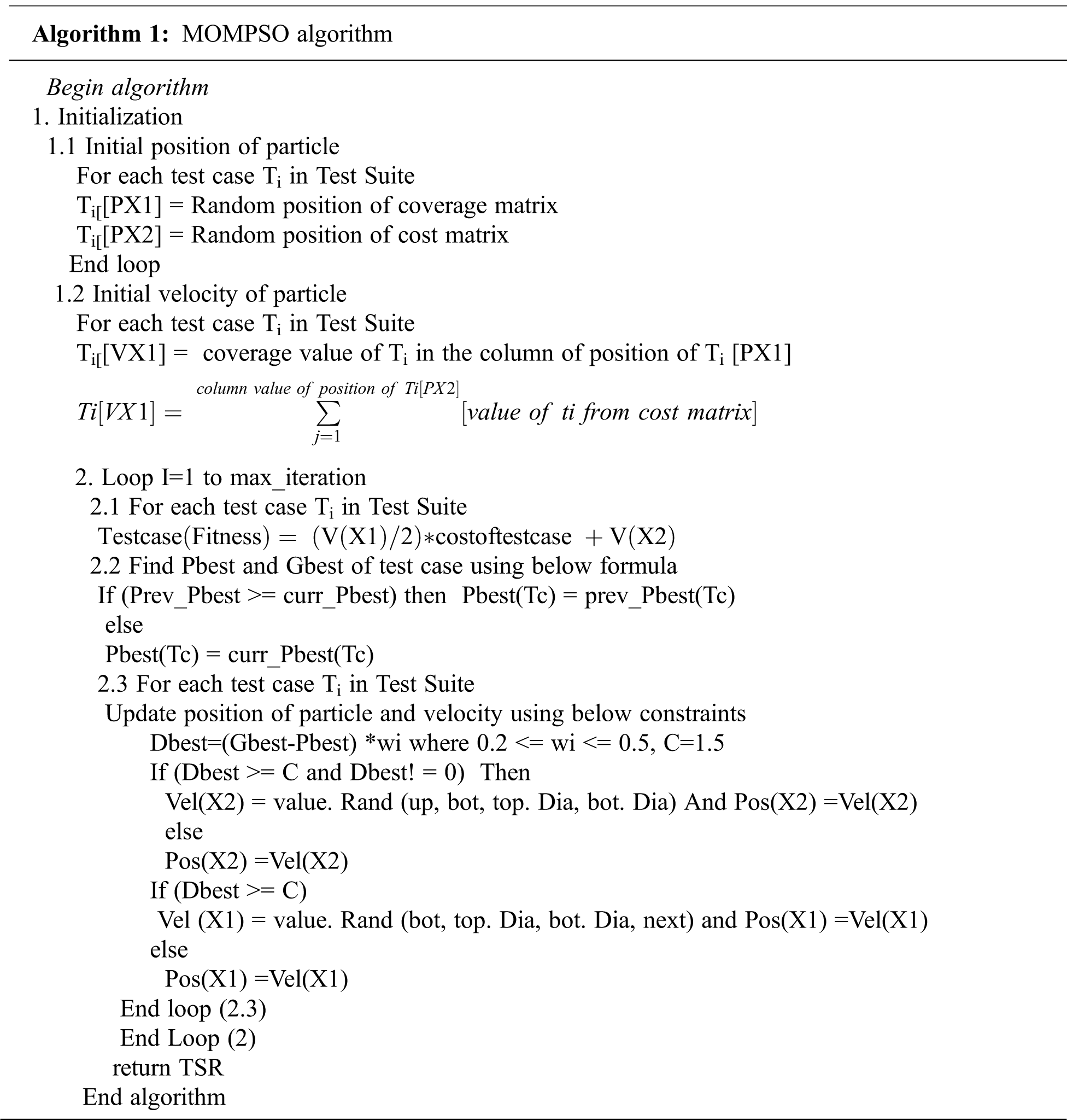
In this section, we present new approach for test suite reduction problem. First, we present a proposed algorithm framework in Section 3.1 second the step by step implementation of MOMPSO is present in Section 3.2. There are two level of algorithm in which first level used for reducing number test cases form larger suite and second level used for reducing number of test cases from smaller suite.
3.1 Proposed Algorithm (MOMPSO)
3.2.1 Test Function and Its Control Flow Graph
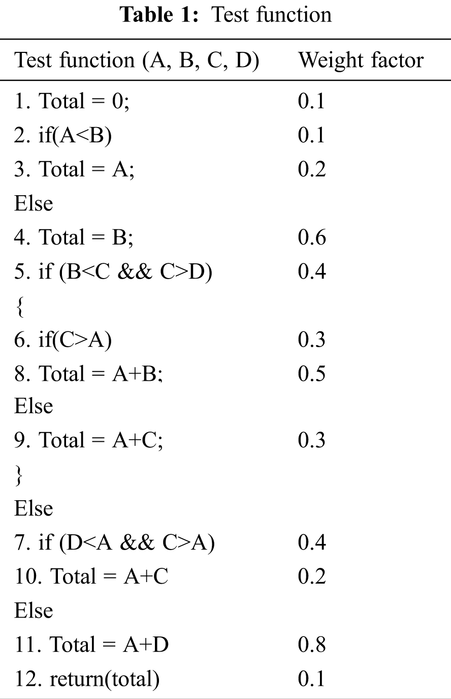
For clarification and validation purposes, this paper considered a test function to illustrate the proposed scheme’s working. This test function is composed of 12 statements, and each information residing in the test function is assigned a random weightage value that lies in a range of 0 to 1. The weight factor assignment to every statement explains the criticality of the data and conditions that these statements are holding (Tab. 1).
3.2.2 Initial Test Suite and Parameters for Test Suite Reduction
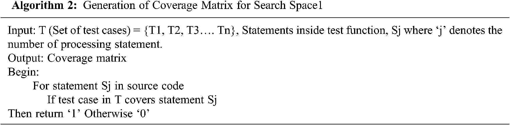
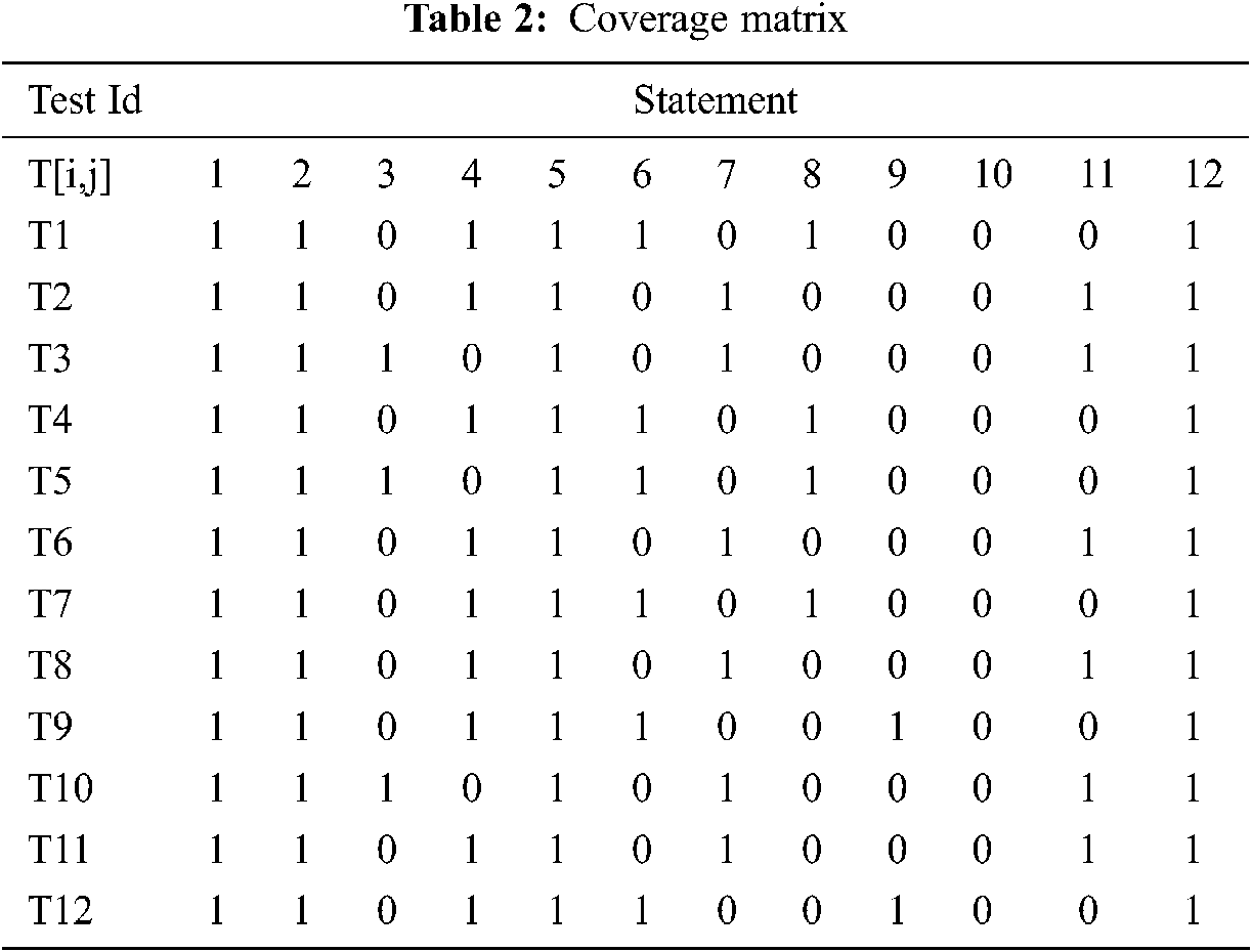
To get started with the methodology, we set up an initial test case pool that consists of all the test cases to be implemented to test the source code (Tab. 1). For this particular case study, ‘12’ test cases are necessitated. We formulated a coverage matrix that indicates the test case coverage value for the corresponding statement. Algorithm ‘2’ elucidates how the values are assigned to each cell present in Tab. 2.
Through the utilization of the coverage information from Tab. 2 [4,21] and the weight factor values from Tab. 1, we calculated the cost involved in processing the whole source code by every test case with the following equation [15,16].
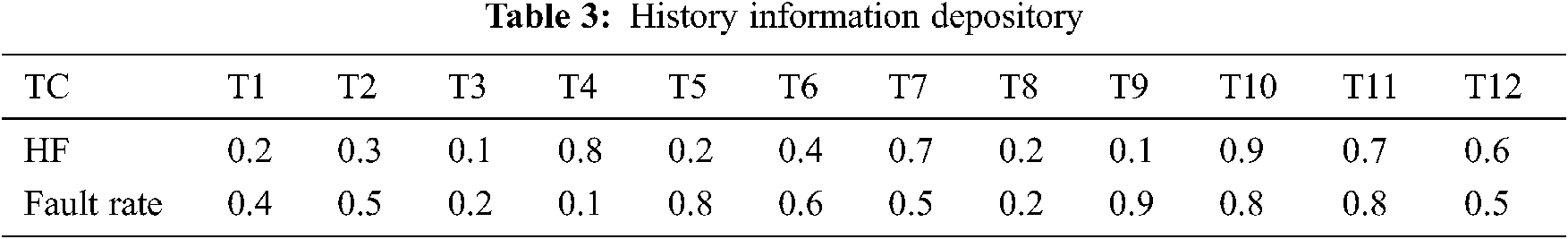
The higher the cost, the most consequential the test case is. Also, a History information depository is maintained, which generally is storage for historical details of every test case in regression testing [4,17,18,21]. It includes the number of times a particular test case is being deployed, the faults disclosed by the test cases, and the severity of detected defects.
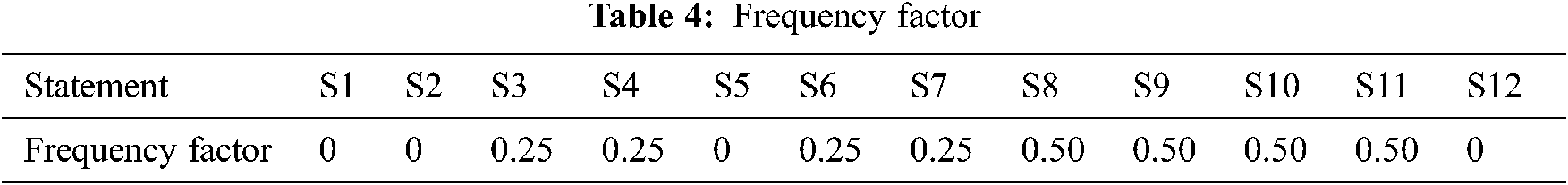
As shown in Tab. 3, the depository displays each test case’s history factor and the test case potentialities of revealing the past defects. With test coverage as one of the essential aspects, understanding how often a single statement is being traversed during execution is also equally important. This notion will present an in-depth view for test cases covering a specific statement that explains that after applying a reduction scheme, the statement that is less frequent and possesses critical data should remain intact with reduced test cases. For example, the frequency factor for statement 1 would be 8/8 i.e.,’1’, which justifies that statement ‘1’ is more frequently appeared in almost all the paths and is of less importance. Therefore, we have taken a value ‘0’ as the final FF for the statements having frequency ‘1’. For less recurrent statements as, in our case, S3 and S4 will have a frequency of ‘0.5’; we considered a slight increment of ‘.25’ for S3 and S4 as contrasted to the final FF value of S1. Moreover, the broad range that we opted for is, if the statement frequency appeared to be equal or more than 50%, then the final FF would be ‘0.25’. Statements with a frequency of less than 50% are allotted a value of ‘0.50’.
As shown in Tab. 4, the equation stated below [19,25].
The coverage matrix’s contribution in knowing which test case covers which statement is a restricted form of information. Also, exploiting only two parameters, i.e., weight factor and test coverage, for quantifying the test cases’ cost will not help in achieving an effective solution. Therefore, we used a multi-objective approach and established another source of valuable data, which is a different manifestation. The matrix format presented in Tab. 5 used the underneath formula to calculate the cost factor of each test case regarding each statement.
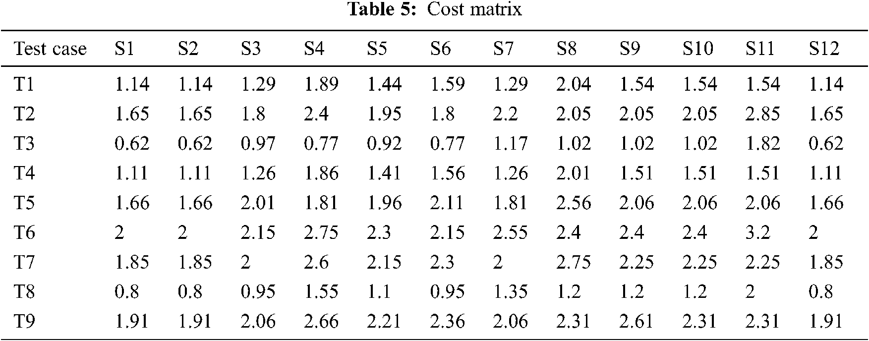
For example: The value of cell (1, 1) is calculated as: cost (T1, S1) = (1*0.9) +0.2+0.4*2.1+0 = 1.14
3.2.3 Experimental Parameter Settings
In the setup, the population size is taken to be ‘12’, which directly denotes the number of test cases. The number of decision variables is decided to be’ 2’ for each iteration, i.e., the coverage and cost matrix, which are also the search spaces for our work. The acceleration factor curbs the distance progressed by the particle (test case) in the iteration. This paper considered the value of acceleration coefficient (C1) to be ‘0’, which illustrates particle movement in a forward manner [12,20,26]. The convergence functioning of PSO is controlled by inertia weight. Initially, we have taken a range of [0.2-0.5] for the inertia weight, though we practiced applying minimum inertia factor while updating the position and population in the search space.
3.2.4 Initial Position and Initial Velocity
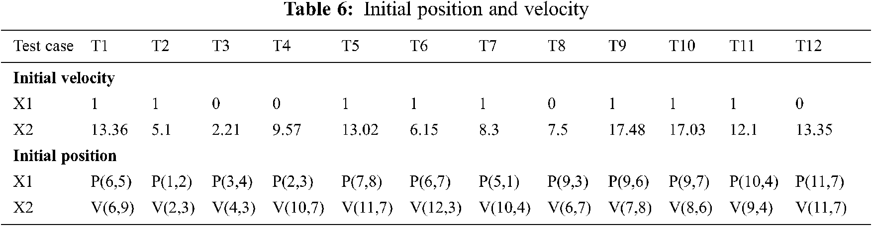
For the first iteration, the population and the velocities are generated randomly. As denoted in Tab. 6, X1 is the representative variable for the coverage matrix, and X2 is the representative variable for the cost matrix. Initially, the particles are randomly dispersed in the coverage search space with certain random positions of velocities, which are mentioned in the cost search space. Cell (T1, X1) with value P (6, 5) highlights the position of test case T1 in the coverage matrix, while cell (T1, X2) with value V (6, 9) denotes the random assignment of velocity position for T1. We followed a systematic order for updating the values for the positions mentioned in the X1 and X2 converted into velocity variable. For updating the values of X1, we referred to the coverage matrix. The cell (T1, X1) of Tab. 8 holds P (6, 5), which ideally points to cell (T6, S5) of coverage matrix. As the location (T6, S5) decodes the fact of test coverage by T6 for statement S5, we checked the coverage of processing test case, i.e., T1 in context to the same statement indicated in the index, that is, S5. Since the cell (T1, S5) holds the value ‘1’, this value is then updated to the cell (T1, X1) of the velocity table. Once column X1 is fed with the updated values for all the test cases, the cost matrix is referred for further processing in the X2 column. The value in cell (T1, X2) of the population table directly signalizes the cost matrix’s cell (T6, S9). The index (T6, S9) describes the cost of test case T6 in connection with S9, and hence, we aggregated the cost from statement 1 to statement 9 of T1 (processing test case). After summation, the value acquired will be the updated value for the cell (T1, X2) of Tab. 8. Likewise, all values in the X2 column are enumerated.
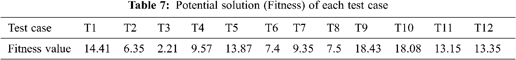
Usually, the fitness function maps the particles’ values to an actual value that must guerdon those particles that are towards an optimal design solution.
During every iteration, the following two best values for each particle is updated. Foremost is the particle’s personal best value (Pbest), which defines the particle’s position in the search space. The next one is Gbest, the global best solution, indicating the best solution among all particles. As the ongoing computation is for the first iteration only, and no previous fitness figures existed, each test case’s current fitness value is the Pbest value. Also, each test case knows the finest value in the group (Gbest) among Pbest. Therefore, as evinced in Tab. 7, 3.11, ‘18.43’ is the procured Gbest value. These Pbest and Gbest values are modified and updated timely after each iteration.
3.2.6 Updating Position and Velocity
After discovering the two prime values, each test case updates its current position and velocity [12]. The modified velocity for each test case can be calculated by using information such as the current velocity and the difference or distance from the Pbest to Gbest. For ensuring whether the distance obtained after applying the formula
Compared with the value of ‘C,’ the Dbest of T2 appeared to be sizeable, which is a direct indicator that the particle’s velocity needs to be modified. This improvement will consider the cost search space. The current velocity position of T2 is V (2, 3) from the initial population table. The cell corresponding to the index V (2, 3) in cost search space holds the value ‘1.85’. This cell demonstrates the current velocity position for test case T2, i.e., T2 from this position can move indiscriminately to directions such as top, bottom, diagonal or next, with the compulsion that every movement should make the test case even closer to the target. We observed that the motion of T2 towards its next direction is a more optimal decision. Consequently, we updated the cell position of T2 in the X2 column of the population table, i.e., the altered velocity position for T2 now becomes V (2, 4). We considered movingT2 towards the bottom direction, and then the location of T2 is updated into the cell (T1, X1) of Tab. 7, i.e., P (2, 2). Furthermore, the fitness computation procedure for the second iteration will be similar to the initial iteration.
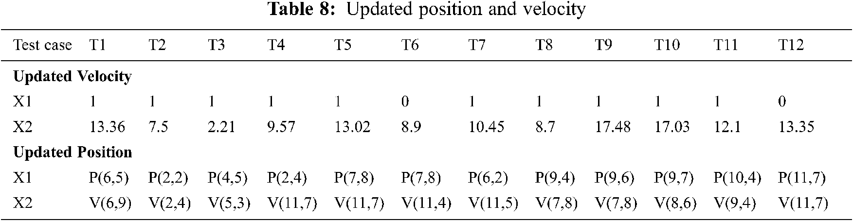
After this iteration, the Pbest and Gbest values of test cases are again inspected. Tab. 8 depicted that the Gbest value remains the same, while the Pbest value of each test case is modified according to the following rule:
If prev_Pbest>=curr_Pbest then Pbest=prev_Pbest else Pbest=curr_Pbest
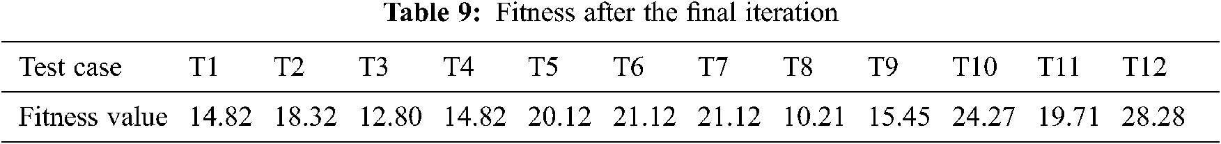
This process of updating the particle’s fitness, current position and velocity until it reaches close to the target continues until the final iteration [12,17,18]. The values for fitness attained by the particle are documented in Tab. 9.
Since the maximal generation has arrived, the particles close to the global best value are extracted from Tab. 9. As mentioned earlier, we set a norm of selecting ‘6’ most prominent test cases out of ‘12’, Reduced Test suite will have following set of test cases.
RTS= {T5, T6, T7, T10, T11, T12}.
RQ1: List some of the advantages with effectiveness for using the proposed algorithm in terms of rate of increase in time, number of reductions of test-cases and overall efficiency of any testing process [15,19].
The Figs. 1 to 6 indicates that proposed approach is more appropriate one for reduction problem. Moreover, it is observed and estimated that the proposed method is much more effective when the calculated sets compared with number of ties is more. As per Figs. 1 to 6, proposed approach decreases no of test cases in test suite and increases coverage, cost, fault rate and overall efficiency of testing process. By considering the result of different application, proposed approach is more efficient for solving test suite reduction problem [4,15,16,32,34].
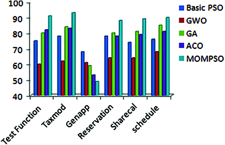
Figure 1: Reduction rate (%)
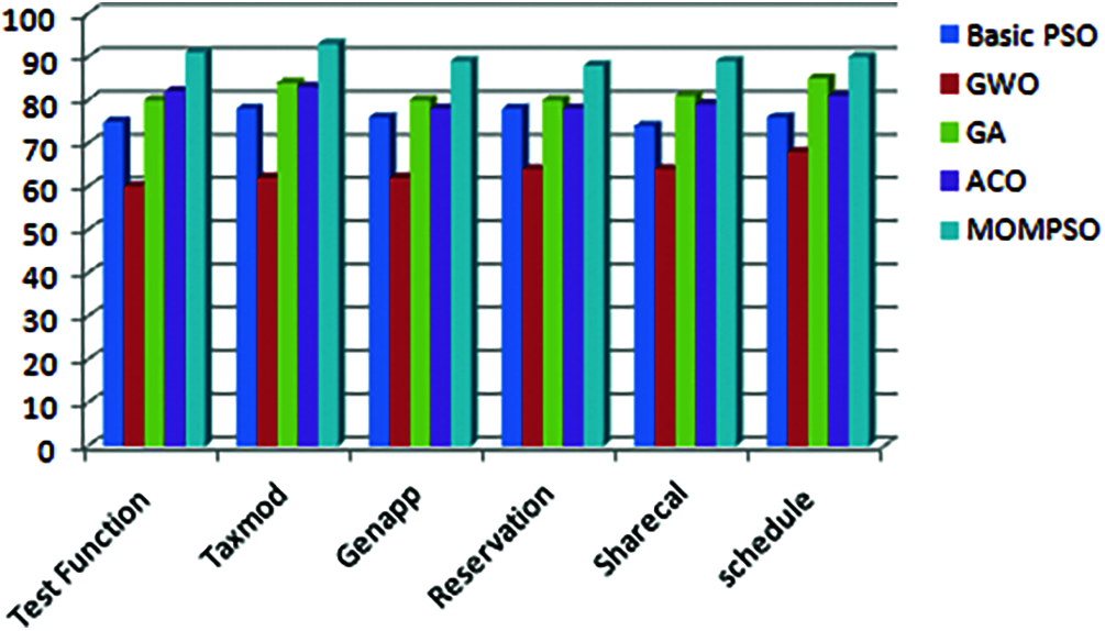
Figure 2: Code coverage (%)
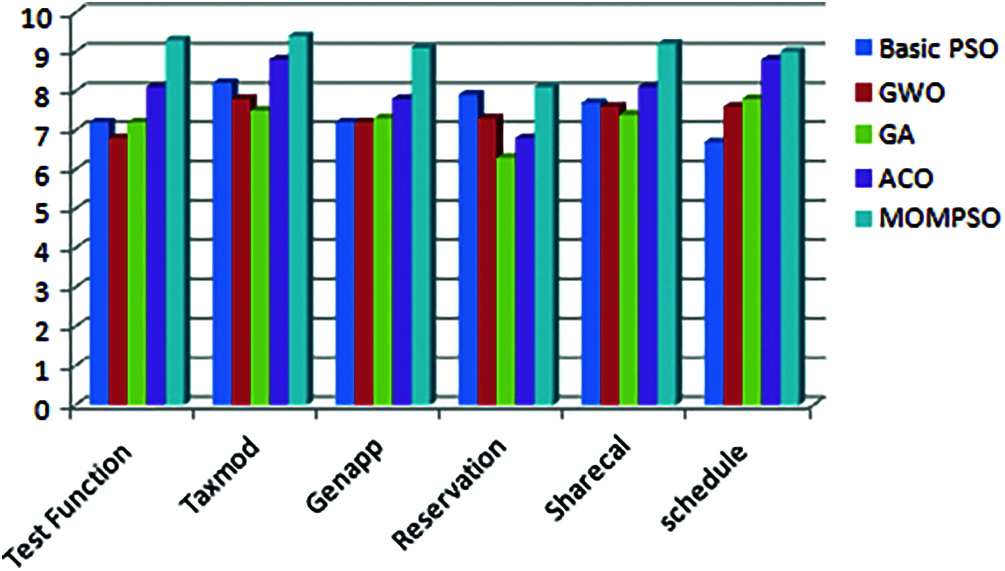
Figure 3: Cost factor
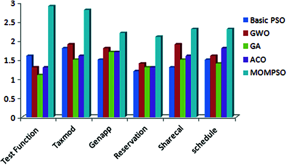
Figure 4: Fault detection Rate
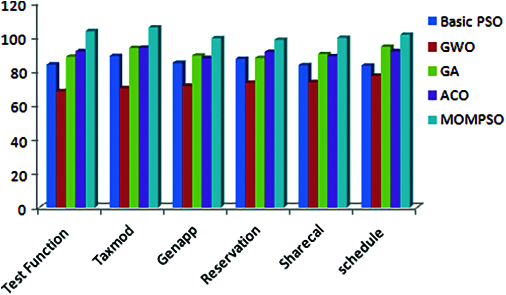
Figure 5: Overall efficiency
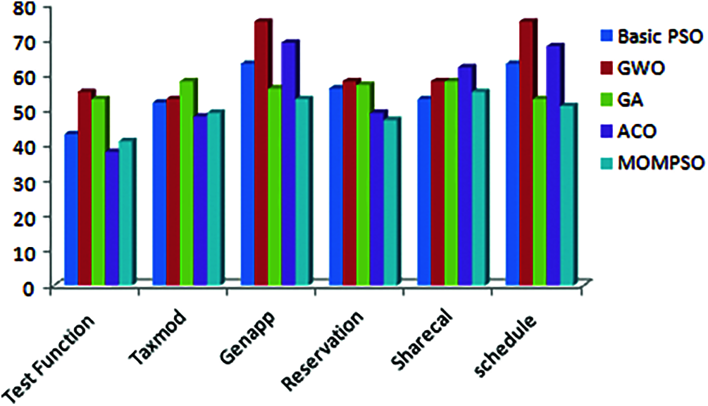
Figure 6: Execution time
RQ2: In the performance parameter of proposed algorithm, list some of the effects with respect to parameter d (depth parameter) [12,15,35].
What are the effects of the depth parameter, d, in the performance of the proposed algorithm?
In terms comparing basic PSO, GWO, ACO, Genetic and MOMPSO, the results show that MOMPSO significantly better than other approach because reduction rate, coverage, cost, history, fault and execution time more effective parameter for test case as well as test suite reduction problem. To increasing the performance of algorithm [15–17,21,25]. MOMPSO uses multiple parameter such as weight, cost of test case, coverage, fitness of test cases and two search space for finding optimal test cases .Due this reason ,parameters which we have considered for reduction algorithm and performance analysis are more efficient for solving test reduction problem [3,17].
4.2 Subject Programs for Testing
Experiments are performed using 6 different open source java programs and the source code is available which can be downloaded with the following link: https://sourceforge.net. This link contains lot of information and earlier studies with prominent literature surveys and reviews regarding selection techniques which prove out to be useful for all the comparative studies performed so far. The average of classification accuracy, fitness function, reduced feature, and computational time for all application using the proposed method are achieved good reduction percentage, coverage, cost, fault and execution time that shown in Figs. 1–6.
4.3 Results for Other Problems
To prove the performance of proposed approach for other than reduction problem, The MOMPSO algorithm tested against 9 standard commercial projects from different open source library, ten instance, 100 number of features has been considered for performance analysis. The parameters of the proposed approach are set as following
• No of particle = 20
• Maximum number of iterations = 100
• Inertia weight is 0.2 to 0.5
All the above values are applied to test the performance of proposed approach. For other algorithm such as ACO, GWO, SI (Swarm Intelligence), Tabu Search and simulated annealing are identical to their own parameter used s.For evolution metrics, information is portioned into three equivalent parts (validation, training, testing) of data. Dividing of data is repeated more no of time to increasing quality of process. The following measures are tested in each run.
• Average of classification accuracy measures set of selected features for more accuracy when algorithm runs N times [16,18].
• Average selected feature (ASF) measures the average selected feature to the overall feature when algorithm runs N times [4,21,35].
• The mean fitness function (MFF) measures average value of fitness achieved when algorithm runs n times [4,22].
• The best fitness function returns the minimum value of fitness when algorithm runs N times.
BF = for I to N min (Fj)
Where Fj = fitness value of j th iteration.
• The worst fitness function returns the maximum value of fitness when algorithm runs N times.
BF = for I to N max (Fj)
Where Fj = fitness value of jth iteration.
As per the results in Fig. 7, classification accuracy of proposed MOMPSO confirms significantly better results than other methods on the majority of the application where MOMPSO provides average number of classification accuracy of 0.871111, while the number of classification accuracy of the SI is 0.802222which is the closest method to our proposed method.
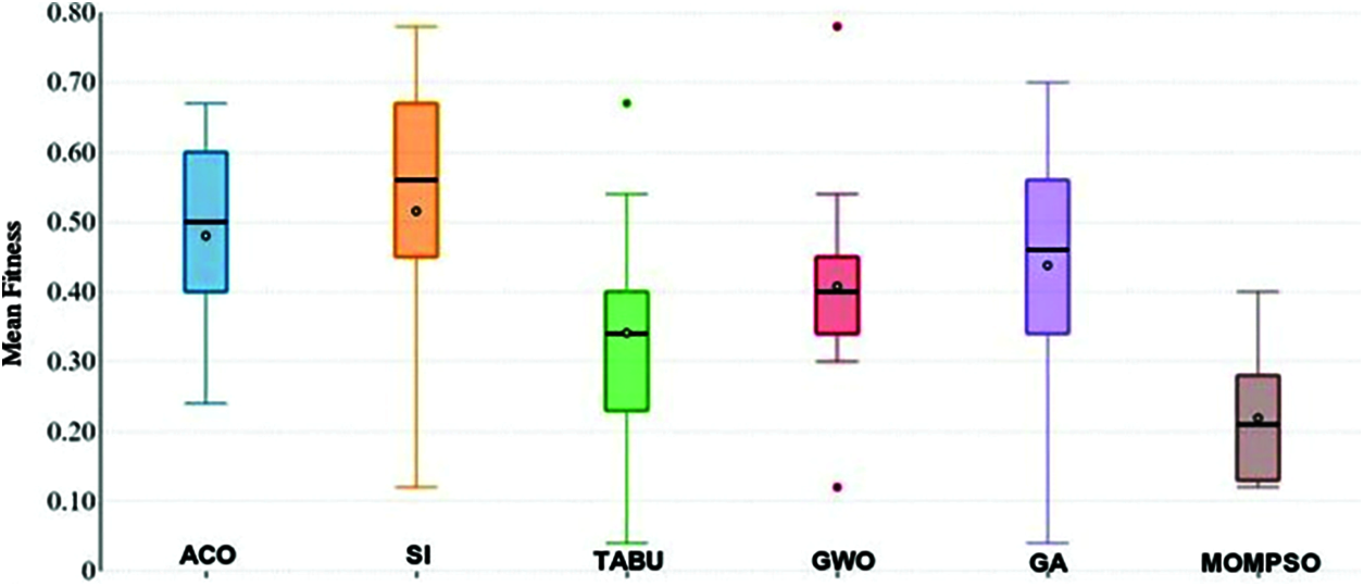
Figure 7: Classification accuracy
According to the results in Fig. 8, the average of selected features of proposed MOMPSO confirms significantly better results than other methods on the majority of the application where MOMPSO provides average number of selected features of 7.253333, while the number of selected features of the SI is 8.437778 which is the closest method to our proposed method.SI approach is closer to other approach as well as proposed approach.
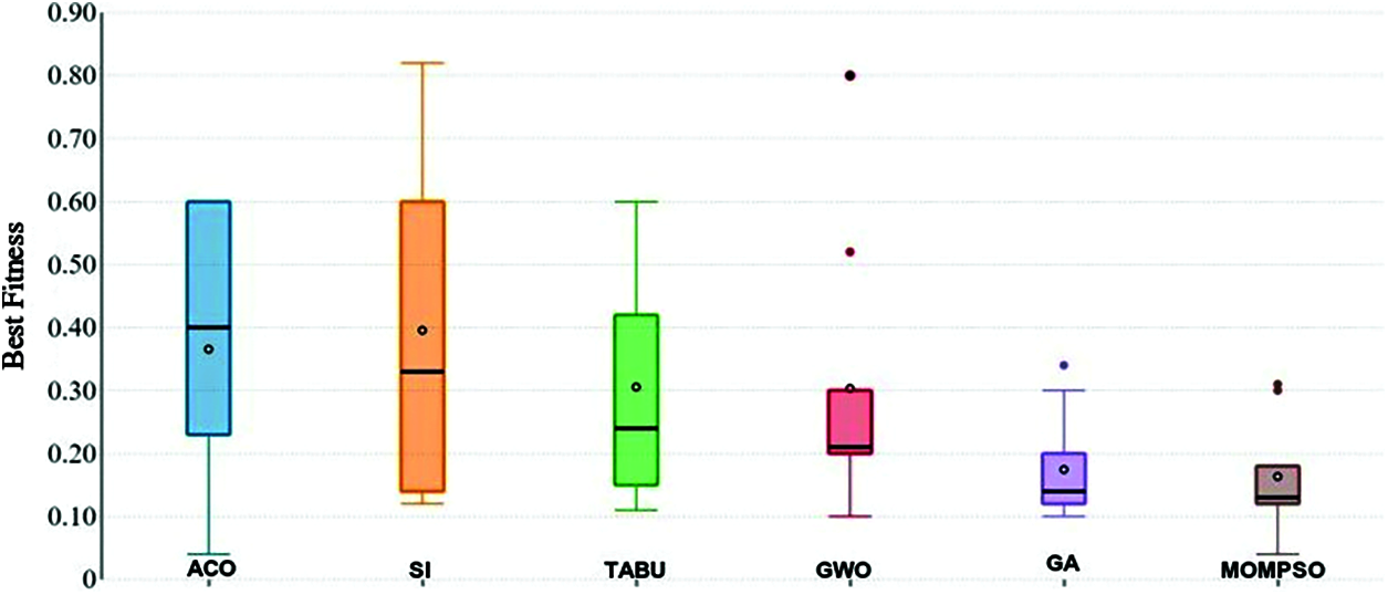
Figure 8: Feature selection
Figs. 9 and 10 shows that the average and best respectively. As per the table, the proposed MOMPSO confirms little bit better results than other methods where MOMPSO provides average number of means, best and worst fitness while the number of fitness of SA is the closest method to our proposed method. In some cases, SI is closest to our proposed approach. At the same SA and Si are close to other method with a minor difference. The good achievement of the proposed MOMPSO method indicates its ability to control the trade-off between the exploitation and exploration during optimization iterations.
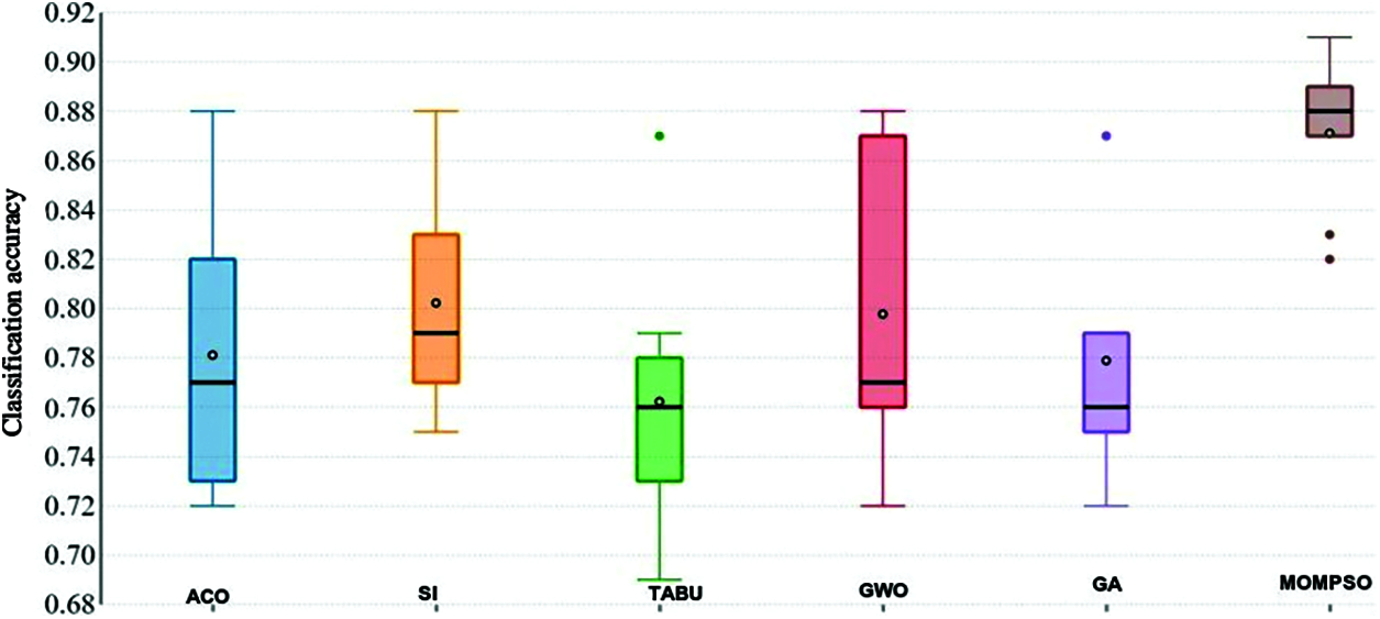
Figure 9: Mean fitness
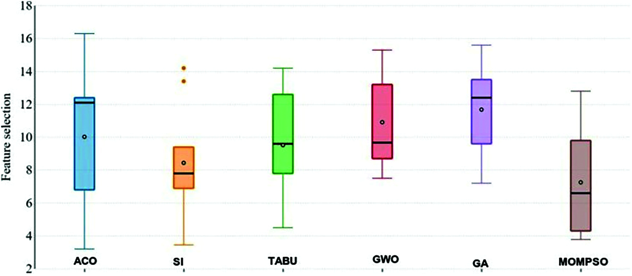
Figure 10: Best fitness
4.4 Result for Few More Reduction Problems
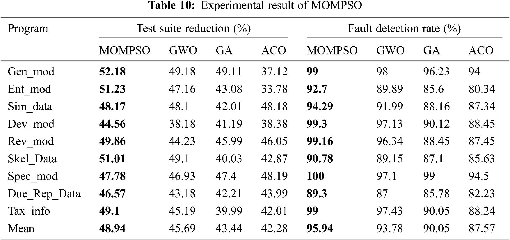
To prove RQ1 and RQ2, Tab. 10 provides different parameter for calculating efficiency of different approach. Figs. 11 and 12 presents box plots of the experimental results. Here box plot gives the mean (square), median(line) and upper and lower quartile (percentage range) for the techniques.
• In MOMPSO method, the reduction rate of sim_data is 48.17 % and it is 48.10% for GWO method. Compared with the GWO method, the proposed method only has a slightly lower reduction rate for sim_data, but difference is only 0.7%. Compared with other method, the MOMPSO method has highest average reduction rate of various method is in Fig. 11 which also answers the RQ1 and RQ2.
• For failure detection rate, compared with all the methods, the average failure detection rate of MOMPSO is 95.94%, which can detect almost all the error in the program. The failure rate of various method is shown in Fig. 12, which also answer the RQ1 and RQ2.
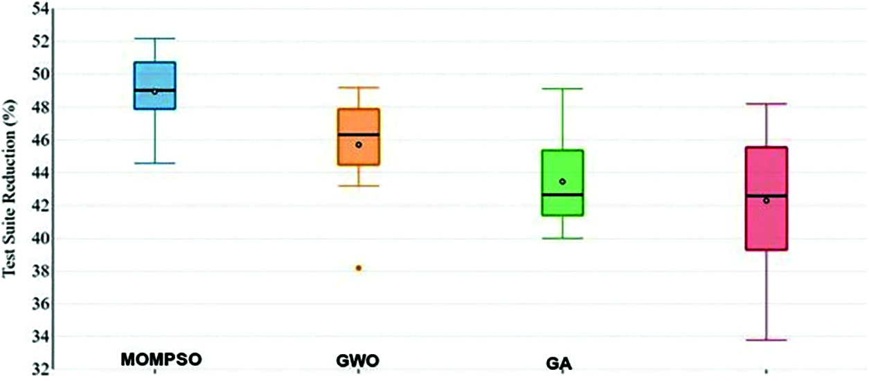
Figure 11: Test suite reductions (%)
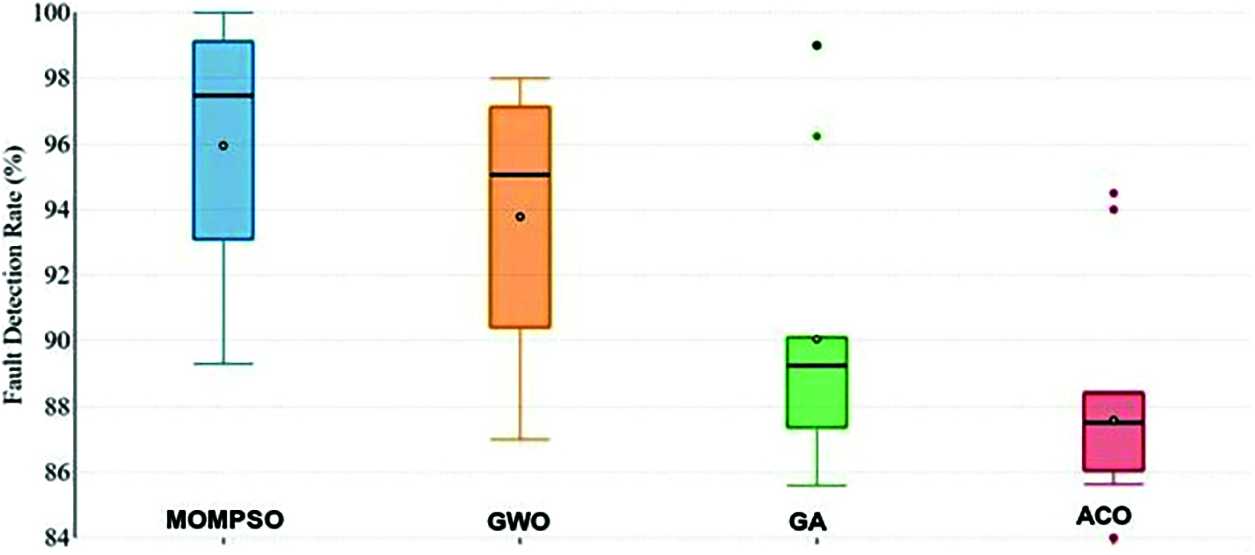
Figure 12: Fault detection rate (%)
5 Conclusions and Potential Direction
It is concluded and estimated that some parameter and single search space for optimization can degrade the performance of various optimization algorithms. To break the issue, multiple parameters and two different dependent search space for test case selection. Most important observation of the newly proposed technique is its efficiency to handle multiple parameters and two different search spaces to find optimal solution. A lot of observation and study is performed simultaneously in order to arrive at the conclusion of using newly derived algorithm (MOMPSO) we propose Modified PSO algorithm for test suite reduction and select test cases from larger test suite and also this approach more useful when we have smaller test suite. In order to get the degree of performance with newly proposed algorithm a continuous study with different cases are performed and then evaluation is done based on comparative study including set of different programs.
In future, the fault history information for version specific regression testing, and the severity of the faults can be jointly considered to improve multi objective optimization for reduction process. Different heuristic approach can be framed, each regarding an independent objective. Then, the different heuristics are multiplied to get more optimal one. Additionally, this research is observed that when the correlation between the sets and test-cases are not handled properly then the performance gets hampered and is not desirable. Potential direction is to handle the issue with a newly proposed algorithm based on correlation value bounded with the performance parameter within the technique.
Funding Statement: The authors received no specific funding for this study.
Conflicts of Interest: The authors declare that they have no conflicts of interest to report regarding the present study.
1. H. Wang, B. Du, J. He, Y. Liu and X. Chen, “IETCR: An information entropy based test case reduction strategy for mutation-based fault localization,” IEEE Access, vol. 8, pp. 124297–124310, 2020. [Google Scholar]
2. R. Huang, W. Sun, T. Y. Chen, D. Towey, J. Chen et al., “Abstract test case prioritization using repeated small-strength level-combination coverage,” IEEE Transactions on Reliability, vol. 69, no. 1, pp. 349–372, 2020. [Google Scholar]
3. I. Alsmadi and S. Alda, “Test cases reduction and selection optimization in testing web services,” Int. Journal of Information Engineering and Electronic Business, vol. 4, no. 5, pp. 1–8, 2012. [Google Scholar]
4. J. Bruce and T. S. Prabha, “A survey on techniques adopted in the prioritization of test cases for regression testing,” Int. Journal of Engineering & Technology, vol. 7, no. 6, pp. 243–275, 2018. [Google Scholar]
5. S. K. Mohapatra and S. Prasad, “Test case reduction using ant colony optimization for object oriented program,” Int. Journal of Electrical and Computer Engineering (IJECE), vol. 5, no. 6, pp. 1424–1432, 2015. [Google Scholar]
6. G. Kumar, V. Chahar and P. K. Bhatia, “Software test case reduction and prioritization,” Journal of Xi’an University of Architecture & Technology, vol. 12, no. 7, pp. 934–938, 2020. [Google Scholar]
7. S. Jeyaprakash and Alagarsamy, “A distinctive genetic approach for test-suite optimization,” in Int. Conf. on Soft Computing and Software Engineering, Berkeley, 2015. [Google Scholar]
8. M. Alian, D. Suleiman and A. Shaout, “Test case reduction techniques–survey,” Int. Journal of Advanced Computer Science and Applications, vol. 7, no. 2, pp. 264–275, 2016. [Google Scholar]
9. Y. Bian, Z. Yi, R. Zhao and D. Gong, “Epistasis based ACO for regression test case prioritization,” IEEE Transactions on Emerging Topics in Computational Intelligence, vol. 1, no. 3, pp. 213–223, 2017. [Google Scholar]
10. D. D. Nucci, A. Panichella, A. Zaidmana and A. D. Lucia, “A test case prioritization genetic algorithm guided by the hypervolume Indicator,” IEEE Transactions on Software Engineering, vol. 46, no. 6, pp. 674–696, 2020. [Google Scholar]
11. A. Bajaj and O. P. Sangwan, “A systematic literature review of test case prioritization using genetic algorithms,” IEEE Access, vol. 7, pp. 126355–126375, 2019. [Google Scholar]
12. M. Khatibsyarbini, M. A. Isa, D. N. A. Jawawi, H. Nuzly, A. Hamed et al., “Test case prioritization using firefly algorithm for software testing,” IEEE Access, vol. 7, pp. 132360–132373, 2019. [Google Scholar]
13. Bestoun and S. Ahmed, “Test case minimization approach using fault detection and combinatorial optimization techniques for configuration-aware structural testing,” Engineering Science and Technology, vol. 19, no. 5, pp. 737–753, 2019. [Google Scholar]
14. S. Renu, “Test suite minimization using evolutionary optimization algorithms: Review,” Int. Journal of Engineering Research & Technology (IJERT), vol. 3, no. 6, pp. 2086–2091, 2013. [Google Scholar]
15. G. Kumar and P. K. Bhatia, “Software testing optimization through test suite reduction using fuzzy clustering,” CSI Transactions on ICT, vol. 1, no. 3, pp. 253–260, 2013. [Google Scholar]
16. I. A. Osinuga, A. A. Bolarinwa and L. A. Kazakovtsev, “A Modified particle swarm optimization algorithm for location problem,” in IOP Conf. Series: Materials Science and Engineering, China, pp. 76–81, 2019. [Google Scholar]
17. M. Ananthanavit and M. Mulin, “Radius particle swarm optimization,” in Computer Science and Engineering Conf. (ICSEC) series, India, pp. 38–43, 2013. [Google Scholar]
18. G. Singh, M. K. Rohit, C. Kumar and K. Naik, “Multidroid: An energy optimization technique for multi-window operations on OLED smartphones,” IEEE Access, vol. 6, no. 6, pp. 31983–31995, 2018. [Google Scholar]
19. N. Sethi, S. Rani and P. Singh, “Ants optimization for minimal test case selection and prioritization as to reduce the cost of regression testing,” Int. Journal of Computer Applications, vol. 100, no. 17, pp. 48–54, 2014. [Google Scholar]
20. M. Kaushal and S. Abimannan, “Automated slicing scheme for test case prioritization in regression testing,” Int. Journal of Engineering & Technology, vol. 7, no. 4, pp. 5266–5271, 2018. [Google Scholar]
21. AdiSrikanth, N. J. Kulkarni, K. V. Naveen and P. Singh, “Test case optimization using artificial bee colony algorithm,” in ACC, USA, pp. 23–31, 2011. [Google Scholar]
22. Q. Luo, K. Moran, L. Zang and D. Poshyvanyk, “How do static and dynamic test case prioritization techniques perform on modern software systems? An extensive study on GitHub projects,” IEEE Transactions on Software Engineering, vol. 45, no. 11, pp. 1054–1080, 2019. [Google Scholar]
23. T. Muthusamy and K. Seetharaman, “Effectiveness of test case prioritization techniques based on regression testing,” Int. Journal of Software Engineering & Applications (IJSEA), vol. 5, no. 6, pp. 113–123, 2014. [Google Scholar]
24. L. Mei, Y. Cai, C. Jia, B. Jiang, W. K. Chan et al., “A subsumption hierarchy of test case prioritization for composite services,” IEEE Transactions on Services Computing, vol. 8, no. 5, pp. 658–673, 2015. [Google Scholar]
25. S. R. Sugave, S. Patil and E. Reddy, “DIV-TBAT algorithm for test suite reduction in software testing,” IET Software, vol. 12, no. 3, pp. 271–279, 2018. [Google Scholar]
26. W. Ding and W. Fang, “Target tracking by sequential random draft particle swarm optimization algorithm,” in proc. of IEEE Int. Smart Cities Conf. (ISC2USA, pp. 18–23, 2018. [Google Scholar]
27. Y. Jia, W. Chen, J. Zhang and J. Li, “Generating software test data by particle swarm optimization,” in proc. of Asia-Pacific Conf. on Simulated Evolution and Learning, China, pp. 22–28, 2014. [Google Scholar]
28. A. Ansaria, A. Khan, A. Khan and K. Mukadam, “Optimized regression test using test case prioritization,” in Proc. of 7th Int. Conf. on Communication, Computing and Virtualization, India, pp. 52–56, 2016. [Google Scholar]
29. H. Do, S. Mirarab, L. Tahvildari and G. Rothemel, “The effects of time constraints on test case prioritization: A series of controlled experiments,” IEEE Transactions on Software Engineering, vol. 36, no. 5, pp. 593–617, 2010. [Google Scholar]
30. C. T. Tseng and C. Liao, “A particle swarm optimization algorithm for hybrid flow-shop scheduling with multiprocessor tasks,” Int. Journal of Production Research, vol. 46, no. 17, pp. 4655–4670, 2008. [Google Scholar]
31. M. Zemzami, N. E. Hami, M. Itmi and N. Hmina, “A comparative study of three new parallel models based on the PSO algorithm,” Int. Journal for Simulation and Multidisciplinary Design Optimization (IJSMDO), vol. 11, no. 2, pp. 5, 2020. [Google Scholar]
32. H. Wang, M. Yang, L. Jiang, J. Xing, Q. Yang et al., “Test case prioritization for service-oriented workflow applications: A perspective of modification impact analysis,” IEEE Access, vol. 8, pp. 101260–101273, 2020. [Google Scholar]
33. I. Koohi and V. Z. Groza, “Optimizing particle swarm optimization algorithm,” in Proc. IEEE 27th Canadian Conf. on Electrical and Computer Engineering, Canada, pp. 28–33, 2014. [Google Scholar]
34. D. Hao, L. Zhang, L. Zang, Y. Wang, X. Wu et al., “To be optimal or not in test-case prioritization,” IEEE Transactions on Software Engineering, vol. 42, no. 5, pp. 490–505, 2016. [Google Scholar]
35. K. Zhai, B. Jiang and W. K. Chan, “Prioritizing test cases for regression testing of location-based services: Metrics, techniques, and case study,” IEEE Transactions on Services Computing, vol. 7, no. 1, pp. 54–67, 2014. [Google Scholar]
 | This work is licensed under a Creative Commons Attribution 4.0 International License, which permits unrestricted use, distribution, and reproduction in any medium, provided the original work is properly cited. |