DOI:10.32604/csse.2022.023221
| Computer Systems Science & Engineering DOI:10.32604/csse.2022.023221 | |
| Article |
Planetscope Nanosatellites Image Classification Using Machine Learning
Department of Computer Science, College of Computer and Information Sciences, Majmaah University, ALMajmaah, 11952, Saudi Arabia
*Corresponding Author: Mohd Anul Haq. Email: m.anul@mu.edu.sa
Received: 31 August 2021; Accepted: 09 October 2021
Abstract: To adopt sustainable crop practices in changing climate, understanding the climatic parameters and water requirements with vegetation is crucial on a spatiotemporal scale. The Planetscope (PS) constellation of more than 130 nanosatellites from Planet Labs revolutionize the high-resolution vegetation assessment. PS-derived Normalized Difference Vegetation Index (NDVI) maps are one of the highest resolution data that can transform agricultural practices and management on a large scale. High-resolution PS nanosatellite data was utilized in the current study to monitor agriculture’s spatiotemporal assessment for the Al-Qassim region, Kingdom of Saudi Arabia (KSA). The time series of NDVI was utilized to assess the vegetation pattern change in the study area. The current study area has sparse vegetation, and exposed soil exhibits brightness due to low soil moisture, constraining NDVI. Therefore, a machine learning (ML) based Random Forest (RF) classification model was used to compare the vegetation extent and computational cost of NDVI. The RF model has been compared with NDVI in the current investigation. It is one of the most precise classification methods because it can model the complexity of input variables, handle outliers, treat noise effectively, and avoid overfitting. Multinomial Logistic Regression (MLR) was implemented to compare the performance of both NDVI and RF-based classification. RF model provided good accuracy (98%) for all vegetation classes based on user accuracy, producer accuracy, and kappa coefficient.
Keywords: Planetscope; nanosatellites; classification; logistic regression; computer vision
Agriculture is a crucial sector in Saudi Arabia due to the increasing population and significant economic growth [1]. Despite various limitations, such as changing climate, less rainfall, limited water resources, hyper aridity, and scattered cultivatable areas, agriculture has prioritized improving food security and achieving self-dependency [2]. Agricultural activities mainly depend on the availability of water consumed from aquifers (shallow/deep) and seasonal water in an arid area [3]. It also makes it very crucial to estimate the water consumption for planning the water resources. Due to the unavailability of water use at the micro-level, satellite-based GRACE data becomes a vital utility to estimate water extraction. Few studies have discussed the consumption of water concerning irrigation using GRACE are available in the literature. [4] Furthermore, [5] used GRACE data (2002–2016) and to understand the Groundwater Storage Change (GWSC) in Saudi Arabia.
Estimation of crop extent and its interaction with climatic parameters is an emerging and vital research area. The role of geospatial techniques provides a promising commitment to estimating and monitoring agricultural growth, environmental change, and water storage change. Previous studies used MODIS (Moderate Resolution Imaging Spectroradiometer) and Landsat suite (TM 5, Landsat 7 ETM+ and Landsat 8 OLI) to obtain the vegetation extent and change across the globe, e.g., [6–10]. Remote Sensing (RS) based NDVI is a technique that can estimate the extent of vegetation in an area and is a measure of crop health. Some studies analyzed climatic parameters such as temperature and rainfall with vegetation based on Landsat NDVI [9,11–15]; the central issue of these studies was that the comparison made with limited images for different times and low spatial resolution (30 m).
Planet Labs’ PS constellation (175 nanosatellites) revolutionized the RS-based vegetation assessment, see Fig. 1. PS-derived NDVI maps are one of the highest resolution data that can transform agricultural practices and management on a large scale. The NDVI time series data is helpful for farmers, and government authorities use this high-resolution information for sustainable agriculture planning, matching crops with changing environment, and allocating resources such as seeds, fertilizers, and, more importantly, water for significant development. Additionally, these NDVI based maps help any disease in the crops and estimate possible crop yield to ensure food security.
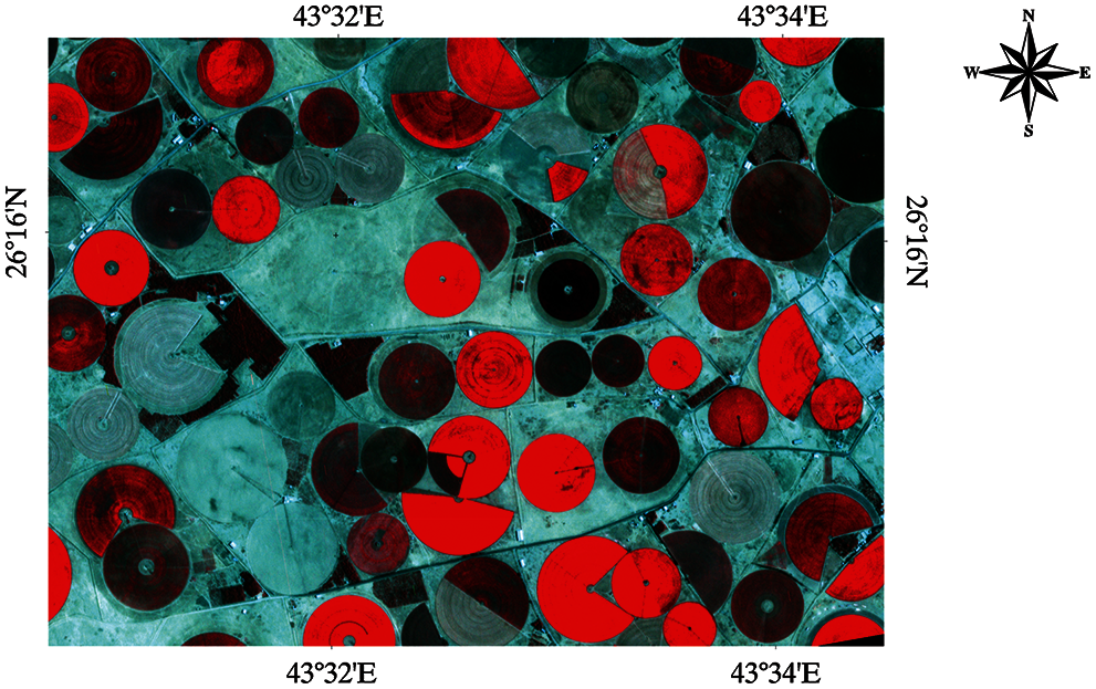
Figure 1: False-color composite of pivot fields using PS subset for Al-Qassim region on April 02, 2021, at 10:34:35
Few studies used PS data for vegetation analysis [16] used PS data and estimated the crop sowing date. [17] use PS data to map Striga weed based on RF. [18] used PS data with other satellite data to monitor crop growth. [19] used ML-based classification to make landuse maps based on PS data and observed an accuracy between 87% and 96%. [20] used PS data to analyze vegetation phenology in Kenya and advocated that the PS images have more detailed NDVI observations due to high spatiotemporal resolution. [21] used PS data and estimated the development stages of winter wheat. [22] fused PS data with Sentinel−2 to classify the vegetation based on NDVI. The research [23] developed an enhancement method to improve the quality of PS data using Landsat 8 and MODIS datasets. The primary issue with the previous study was that the vegetation derived from PS data needs to calibrate the atmospheric correction with other satellites. Another issue was the time series PS observations; some researchers used six months of data while others used 12 months. The present investigation overcame the limitation by using the level 3B surface reflectance products 3B_AnalyticMS_SR.tif and a continuous time series of more than 2.5 years for good insight into crop growth assessment.
Machine learning algorithms generally used in image classification are Artificial Neural Network (ANN), Support Vector Machine (SVM), Random Forest (RF), and Maximum Likelihood Classifier (MLC) [24–27]. [28,29] used the RF algorithm to analyze the sugarcane vegetation. Several studies have logically advocated using Random Forest’s classification for remote sensing data [17,30–33]. RF used several decision trees based on ensemble modeling of training samples and variables. The RF model can process higher dimension data, solve multicollinearity issues, and provide high accuracy with less computation time [10,34]. Almost negligible studies used PS data for RF-based classification. The comparative assessment of any ML model is essential to understand the performance of the model. The novelty of the present investigation is to use MLR between NDVI and RF-based vegetation classification for three categories: high vegetation, low vegetation, and no vegetation.
The assessment of water extraction and the impact of climatic parameters on vegetation is a significant contribution attempted in the present investigation. In the present research, an attempt was made to apply high-resolution PS data and climatic parameters to assess the spatiotemporal assessment of vegetation in the Al-Qassim region in KSA. There are three primary objectives of the current investigation: (1) Monitoring the agricultural pattern change for improved decision-making and sustainable agricultural development; (2) Estimating water extraction based on GRACE and GRACE-FO; (3) vegetation classification using RF model; (4); Performance comparison between NDVI and RF-based vegetation classification using MLR; and (5) Assessing the interaction of vegetation with climate parameters and water extraction.
The novelty of the present investigation is to develop and apply an RF classification model for continuous PS nanosatellite vegetation time series of 28 months, which is the longest continuous time series analysis for nanosatellites images for crop pattern growth and change. Another novelty of the present investigation is to assess the impacts of gravity-based groundwater change and climatic parameters on high-resolution vegetation change.
Al-Qassim region contains almost 1.5 million population and a cultivation area of 1029 km2, making Qassim the third-largest agricultural region, around 12.32% of total KSA in 2009 [35]. The Qassim region is well documented in earlier work for vegetation change [36]. The primary cultivar is dates, wheat, and clover, representing approximately 40.35%, 23.39%, and 15.18% of the cultivated area, respectively [37]. Qassim region has a hot desert climate and rainfall around 93.44 mm.
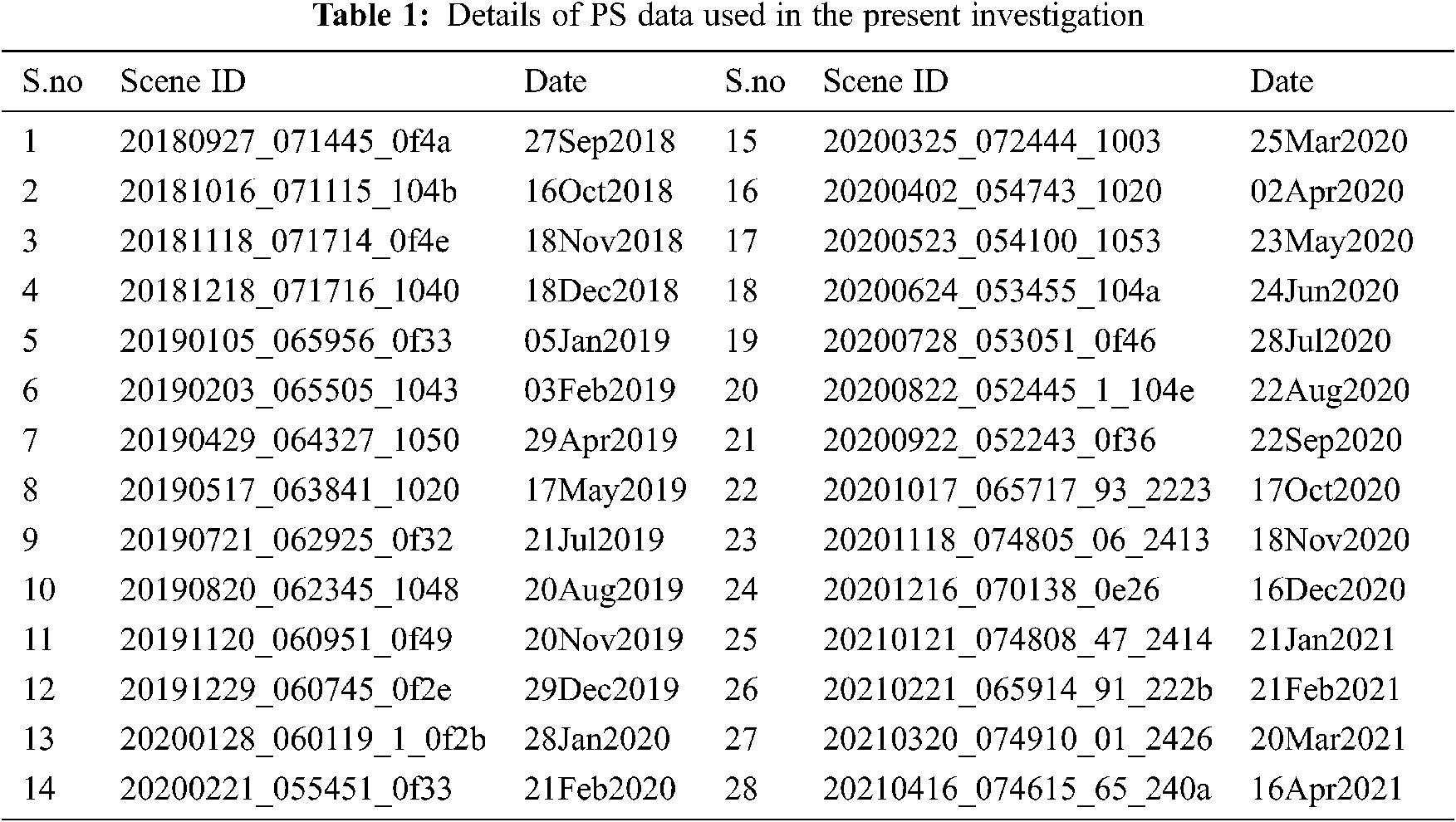
A total of 29; level 3B surface reflectance products (3B_AnalyticMS_SR.tif) supplied by Planet Labs were used in the present investigation, see Tab. 1. It was worth noting that the very high spatial resolution of PS 3 (m) and temporal resolution of 1 day make it suitable to assess the vegetation pattern with high accuracy. The surface reflectance product (SR-Planet Surface Reflectance Product) involves various quality checks, corrections including atmospheric correction [38], were utilized directly in the present investigation. The present investigation captures the vegetation details through PS nanosatellites from September 2018 to April 2021 (28 months) with gaps for 2019 and March, June, September, and October (4 months).
Terrestrial water storage (TWS) was obtained from GRACE and GRACE-FO satellites from Sep 2018 to April 2021 monthly temporal and half degree spatial resolutions. GRACE release 06 (RL06) V 2.0 global mass concentration blocks or mascon products were used in the present investigation, acquired from CSR (Center for Space Research at the University of Texas, Austin) and Jet Propulsion Laboratories (JPL).
The Modern-Era Retrospective analysis for Research and Applications, Version 2 (MERRA-2) was downloaded from (https://gmao.gsfc.nasa.gov/reanalysis/MERRA-2/). MERRA-2 contains average temperature (Tavg), temperature (Tmax), minimum temperature (Tmin), surface temperature (Tsurf), wind speed (WS), and evaporation from Sep 2018 to April 2021 [39]. The rainfall data was downloaded from (https://www.chc.ucsb.edu/data/chirps) with a resolution of 0.05°. CHIRPS data is derived using satellite imagery and in-situ data [40].
GRACE does not distinguish between anomalies from several elements of TWS (Terrestrial Water Storage) contained in surface water storage, canopy water, and soil moisture content. Therefore, subtraction of non-groundwater components was required to obtain the GWS. The surface water and canopy water are almost negligible for the current investigation area due to the semi-arid region. Therefore, only the soil moisture content (SMC) must be subtracted from the TWS to obtain the GWS as Eq. (1).
SMC was obtained using the Global Land Data Assimilation System (GLDAS) by averaging the three different LSMs viz. NOAH, CLM, and VIC (https://disc.gsfc.nasa.gov/). The GRACE JPL, CSR, and average data are shown in Fig. 2. The SMC and TWS errors were added in quadrature to obtain the error in GWS [4,41].
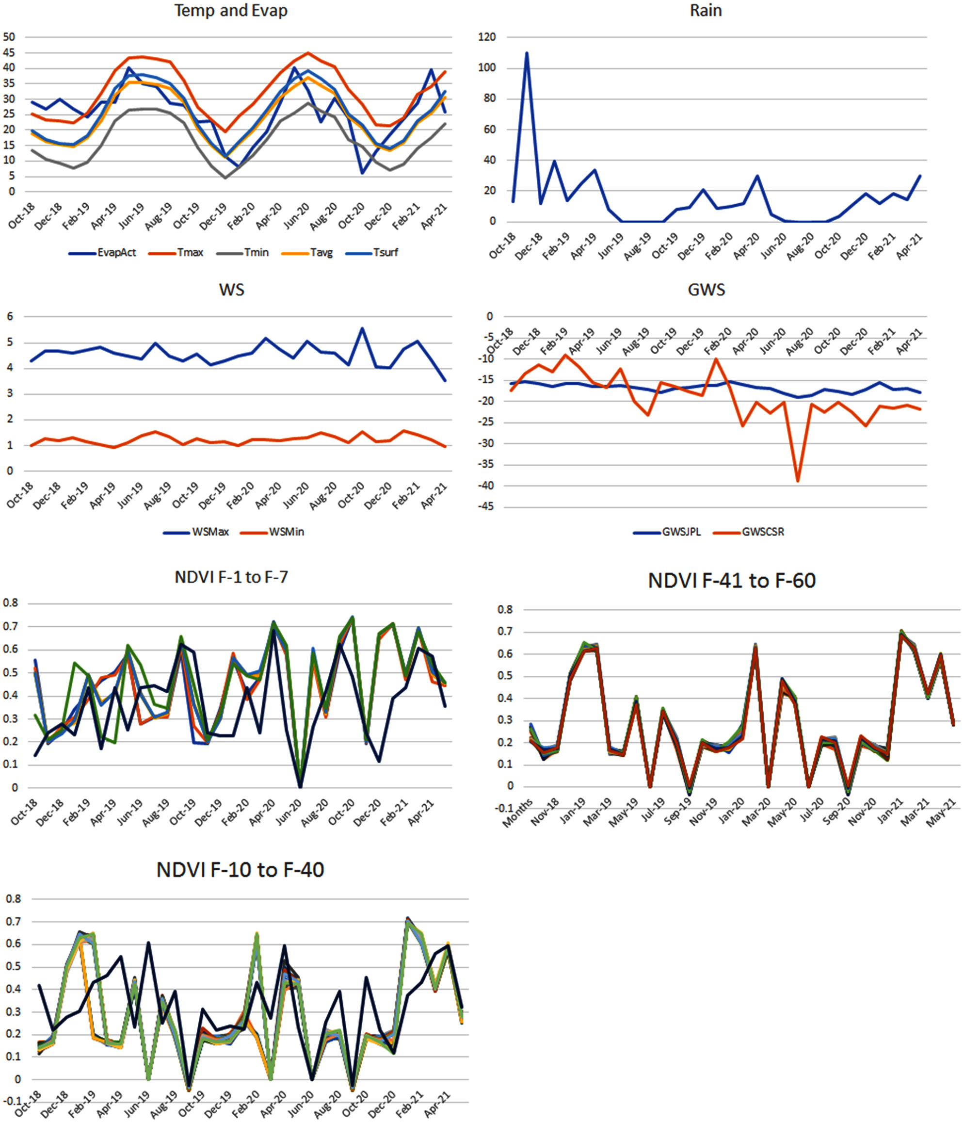
Figure 2: The time-series observations of temp, evaporation, rainfall, windspeed, GWS, and NDVI for 60 pivot fields (F) from Sep 2018 to April 2021
The NDVI index is based on vegetation greenness or the photosynthetic process of vegetation, an index of plant “greenness” or photosynthetic activity [7,9,33]. NDVI used the principle that the vegetation absorbs the red light required for photosynthesis; however, it reflects the NIR light. The non-vegetated areas or stressed vegetation do the reverse process, i.e., the reflection of red light is more, and the NIR region’s reflection is relatively more minor.
NDVI can be obtained from the following Eq (2).
NDVI depends on various factors such as total vegetation cover, soil moisture, and vegetation stress. Being a ratio, NDVI has advantages such as compensation of illumination conditions due to topography and multi-temporal image analysis for comparisons as images collected in different seasons. Fig. 3 illustrates the NDVI of 60 pivot fields.
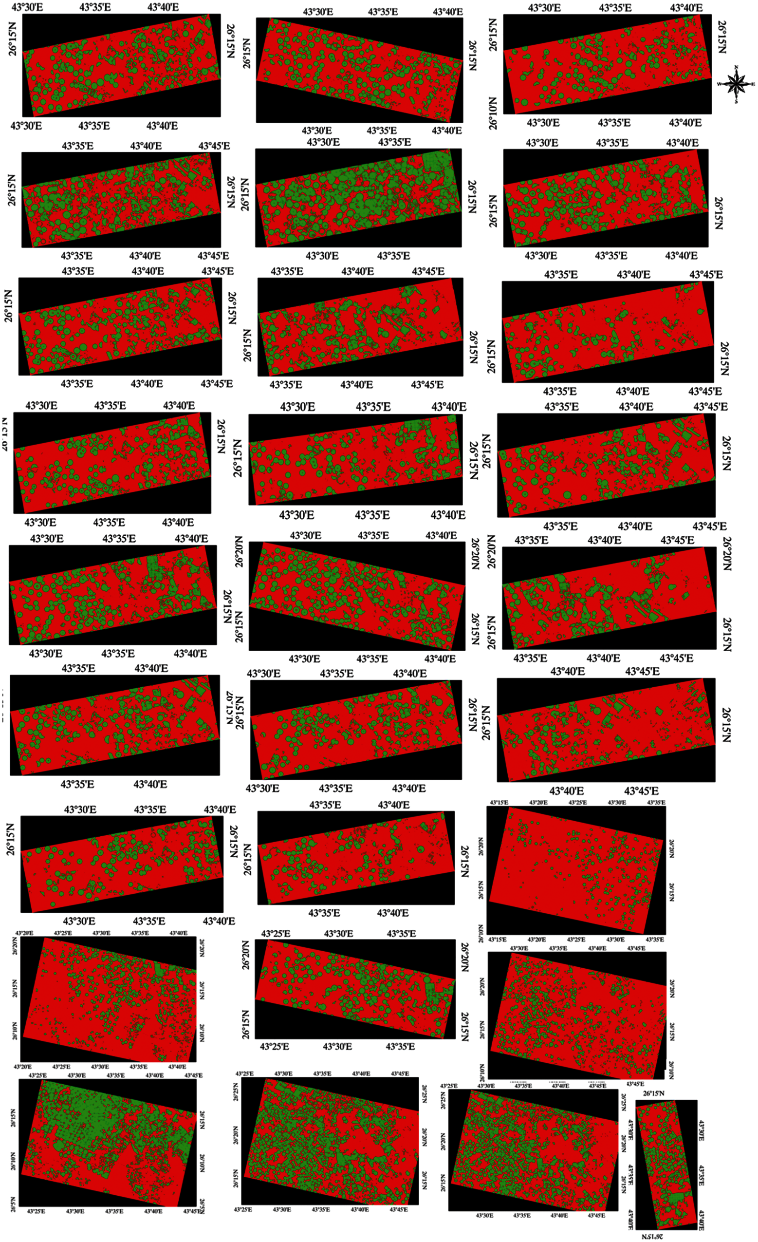
Figure 3: PS images derived NDVI between September 2018 to April 2021. Green color shown vegetation and red color represent no vegetation
4.3 Trend and Correlation Analysis
Mann-Kendall trend tests [42, 43] were carried out for trend analysis to detect trends and changes in vegetation, GWSC, and climate variables over the years of analysis. Sen’s slope values [44] were used to understand the trend of GWSC change for the study area from Sep 2018 to April 2021. The Mann-Kendall S value statistics were evaluated chronologically in the time series (Eq. (3)). The observations VAR(S) variance in the time series was also estimated (Eq (5)). Standardized test Z (Eq. (6)) [45] was also performed for the statistical analyses.
Here, Xi and Xj are chronologically placed values of variables in the time series, n represents the total count of observations, ties for pth value are shown as tp, and tied values number is shown as q. A positive and negative value of Z determined the increasing and decreasing trend, respectively. The Pearson correlation was used to understand the relationships between water extraction (GWSC), NDVI, and climatic parameters for the study area between Sep 2018 and April 2021.
4.4 Random Forest-Based Vegetation Classification
Defining the function was the first step in the RF classification; it defines the required features for data splitting, impurity function, number of samples, and stopping criteria. In this study, the Gini coefficient function was used for RF classification; which can be expressed as Eq. (7):
where; n represents classes, v = vertex of the trees.
A total 300 decision trees were chosen for RF model.
4.5 Multinomial Logistic Regression Between NDVI and RF Model Classification
MLR was applied to find the correlation between NDVI and RF classified vegetation. Logistic regression (LR) is helpful for two categories. For more than two categories, the MLR is applicable; in the present investigation, three classes (high vegetation, low vegetation, and no vegetation) were used in MLR. Multinom function from the nnet package of R Language was applied. The level of the outcome was used as baseline applied through in relevel function. The MLR model was evaluated using stratified k-fold cross-validation, which ensures the class balance for training. Total three repeats and ten folds were selected to evaluate the MLR. The multinom package has no option for p-value calculation for the regression coefficients; therefore, p-values are calculated using z tests.
H0: Null hypothesis: There is no effect of NDVI on the RF-based vegetation classification
H1: Alternative Hypothesis: There is a significant effect of NDVI on the RF-based vegetation classification
The z-statistic was computed using Eq. (10).
where
The null hypothesis was false when the probability value was less than 0.05. The null hypothesis was rejected if the output value was higher than the probability threshold or significance level (α). The null hypothesis was rejected in case the output value was lesser than the α. The α value of 0.05 and the two-tailed z-test were used to reject the null hypothesis. The relationship between NDVI and RF classification was observed as statistically significant when the null hypothesis was rejected.
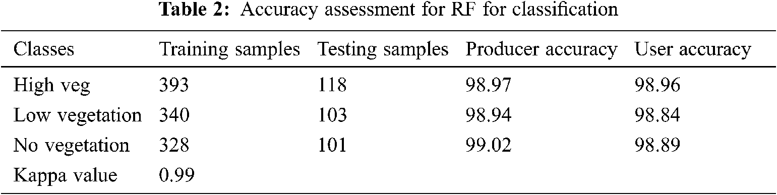
The machine learning algorithm RF was performed for vegetation classification. The classification accuracies were calculated using the confusion matrix. The Kappa statistics were evaluated [46,47].
Cohen’s kappa coefficient (K) [47] is given as Eq. (11)
where N represents measurements. The SMC and TWS errors were added in quadrature to obtain the error (±1.2 mm) in GWS [4,41]
5.1 Extraction of Groundwater Based on GWSC
We have processed GRACE GWSC based on CSR and JPL mascon data for the Qassim region’s identical PS footprint. The highest annual water extraction was observed in Aug 2020 for both GWS based on JPL and CSR. March 2020 and Feb 2021 were observed positive water levels for GWSJPL and March 2019 and February 20 for GWSCSR.
28 PS images were processed between September 2018 to April 2021 for 60 pivot fields, see Fig. 3. Our findings indicated that the agricultural activities were almost similar for 60 pivot agriculture fields analyzed in the present investigation. The 60 pivot fields were categorized into three categories based on NDVI time series behavior. The highest values of NDVI were observed in April 2020 and Jan 2021, whereas the lowest NDVI values were observed for Sep 2019, June 2020, and Dec 2020. The fields from 1 to 7 and 41–60 showed significantly increasing NDVI value from September 2018 to April 2021; the 10 to 40 showed stable trends.
5.3 Trend and Correlation Between Vegetation and Climatic Parameters
The vegetation extent based on NDVI showed an increasing trend for 30 pivot fields with Kendall’s Tau of 0.15 and slope = 0.004. The other 30 pivot fields shown Kendall’s Tau of 0 mean no trend or stable NDVI values. The Kendall’s Tau values for the GWSC change rate were −0.8 mm/year and −0.06 mm/month for GWSJPL. The Kendall’s Tau value for GWSCSR change rate was higher than GWSJPL, i.e., −1.6 mm/year and −0.12 mm/month for GWSCSR. The monthly rainfall showed a decreasing trend with Kendall’s Tau of −0.60 and a slope of −0.01 based on CHRIPS gridded data. The highest monthly rainfall (110 mm) was observed during Nov 2018. The months from Jun-Oct shown no rainfall whereas April month showed higher rainfall during all three years. The annual rainfall for the years 2019 and 2020 was 149 mm and 194 mm. The Tmax was higher (45°c) during May-June, and Tmin was lower during winters (5°c). The temperature, wind speed, and evaporation trends were stable; additionally, the evaporation perfectly aligned between Tmin and Tmax. The highest ws was observed during Oct-20.
Some studies analyzed the climatic impact on vegetation, especially using NDVI [13,16–18]. An attempt was made to study the impact of climatic parameters such as temperature and rainfall on vegetation, see Fig. 4. The PME MET station rainfall data was available for only one study area from 2009–2018 with gaps; additionally, one station can cover 10 km2 [45]. Therefore, the latest CHRIPS and MERRA-2 datasets were utilized in the present investigation. The present investigation found interesting interactions between vegetation, environment variables, and water extraction. A correlation was also found between environment variables. The rainfall showed a correlation of 0.47 with reference evaporation. The correlation of rainfall with GWSJPL and GWSCSR was 0.38 and 0.26, respectively indicate that GWSJPL has shown a better relationship with rain than the GWSCSR. The rainfall and temperature (Tmax, Tmin, Tavg, and Tsurf) showed correlation values of −0.35, −0.33, −0.34, and −0.33. The rainfall and NDVI of 10 pivot fields correlated between 0.13 and 0.22, which is not strong. Actual evaporation showed a strong relationship with the R-value of 0.62 for all four temperature variables, while reference evaporation showed a significant relationship with temperature variables (r≥0.93). Reference evaporation signifies water extraction with an R-value of −0.53 and −0.43 for GWSJPL and GWSCSR, respectively. The average correlation value of vegetation with reference evaporation shown a correlation value of 0.37. The water extraction based on GWSJPL and GWSCSR showed a significant correlation of 0.38 and 0.40 for almost 90% of pivot agriculture fields discussed in the present investigation. GWSJPL and temperature relationship was significantly shown an R-value of 0.41. GWSCSR showed a correlation of 0.31 with temperature. The R-value of GWSCS and vegetation for the majority of pivot fields were 0.27. The wind speed had a weak relationship with NDVI ranging between 0.15 to 0.20. The relationship between NDVI of all pivot fields = 0.93 signifies that all pivot fields follow the same agricultural practice.
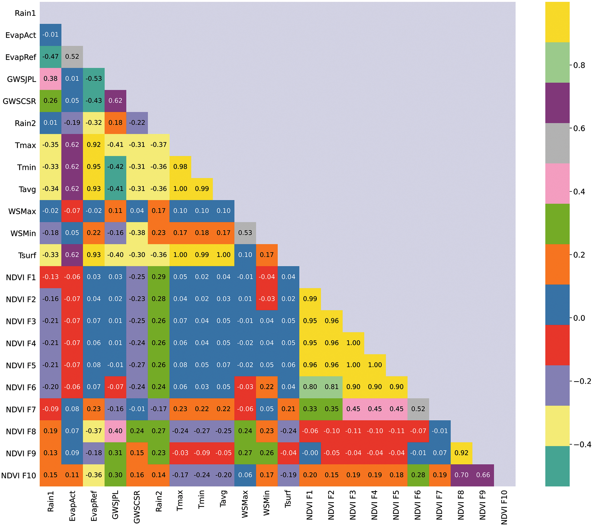
Figure 4: Correlation plot between climatic parameters and the NDVI of 10 pivot fields
RF provided good accuracy for all three classes, i.e., high vegetation, low vegetation, and no vegetation, based on user accuracy, producer accuracy, and kappa, see Fig. 5. This method performed admirably in vegetation identification with higher producer and user accuracy. The error margin was relatively low, see Tab. 2. The RF is one of the most precise classification algorithms due to its ability to model the complexity of input variables. It can handle the noise and outliers as exposed soil in the current study, leading to indices’ saturation. As a result, the results obtained from RF are generally better than other ML classification algorithms.
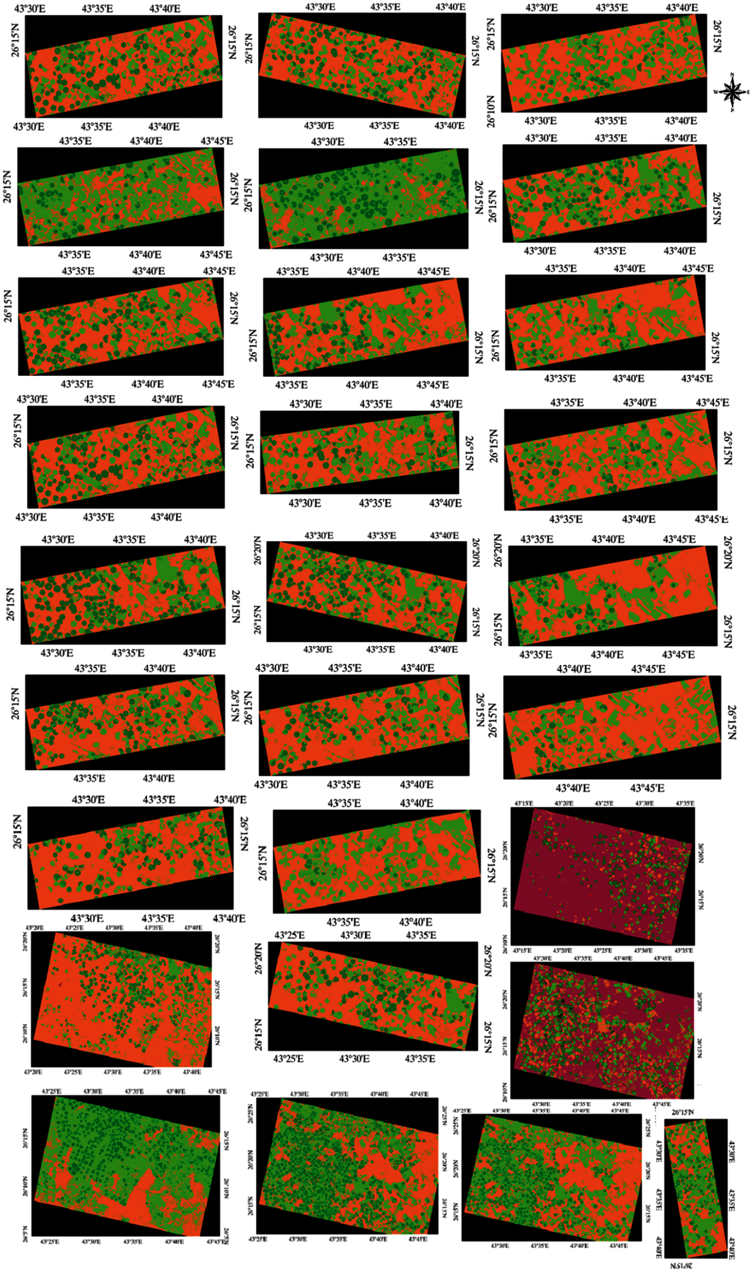
Figure 5: RF Classification on PS images between September 2018 to April 2021. Dark green color represents high vegetation; light green color represents low vegetation, maroon and thistle color represent no vegetation
5.5 Multinomial Regression Results
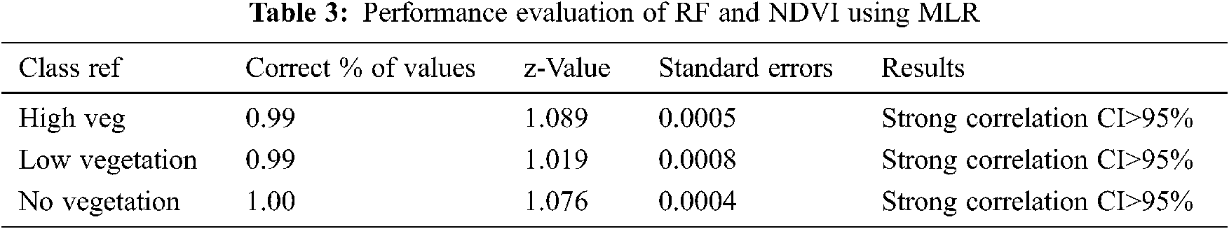
An attempt was made to evaluate the performance of vegetation classification between NDVI and RF. The correlation results for all three classes are given in Tab. 3. All three classes showed a strong correlation between NDVI values and RF-based vegetation classification. The z-value is below −1.96, and the p-value is < 0.05 for all three classes; therefore, it can be concluded that there is a strong correlation between NDVI and RF, so the null hypothesis is rejected. The results indicated that NDVI and RF had shown almost similar results, further confirmed through 30 random points using sub-meter resolution’s Google Earth Image dataset for available months between Sept 2018 and April 2021.
Accurate vegetation knowledge over a high resolution (3 m) can be achieved using revolutionary nanosatellites datasets such as Planetscope (PS) for understanding the agricultural sprawl. According to the changing climate, it is significant to understand the interaction of climatic parameters and water requirements with vegetation on a spatiotemporal scale to achieve sustainable crop practices. In the present investigation, high-resolution PS nanosatellite data was utilized to assess the spatiotemporal assessment of agriculture for the Al-Qassim region, KSA. For this purpose, the time series of NDVI was used for 29 months of time series data. The present investigation used the GRACE and GRACE-FO data to estimate the water used for vegetation. RF model was used to classify the vegetation, and MLR was applied to compare NDVI and RF-based classification performance.
The present investigation found interesting interactions between vegetation, environment variables, and water extraction. Rainfall and water extraction through GWSJPL showed an R-value of 0.38, while reference evaporation showed an R-value of −0.53 with GWSJPL. Temperature and GWSJPL showed a significant relationship with an R-value of 0.41. Among all climatic parameters, reference evaporation showed a good relationship with NDVI of all fields with an R-value of 0.37. GWS has also shown a good relationship with all 60 pivot fields with an R-value of 0.4. The correlation of rainfall with GWSJPL and GWSCSR was 0.38 and 0.26, respectively indicate that GWSJPL has shown a better relationship with rain than the GWSCSR. The future scope of the present research will be to utilize other high-resolution datasets and extend the study area with additional datasets such as soil moisture models to understand the agricultural pattern with different climatic parameters and techniques [48,49]. The selection of crop type and harvesting time should be compatible with the changing environmental conditions and water availability to achieve sustainable agriculture. Future agricultural practice depends on making informed decisions using high-resolution temporal assessment of matching crops according to the environment.
Acknowledgement: The author is thankful to Planet for providing high-resolution PS Nanosatellite data at no cost.
Funding Statement: The author extend their appreciation to the deputyship for Research & Innovation, Ministry of Education in Saudi Arabia, for funding this research work through the project number (IFP-2020–14).
Conflicts of Interest: The author declares that they have no conflicts of interest to report regarding the present study.
1. J. Alam, M. Daoud, S. Magram and R. Barua, “Impact of climate parameters on agriculture in Saudi Arabia: Case study of selected crops,” the International Journal of Climate Change: Impacts and Responses, vol. 2, no. 1, pp. 41–50, 2010. [Google Scholar]
2. R. Samara, “Assessing the applicability of ground penetrating radar (gpr) techniques for estimating soil water content and irrigation requirements in the eastern province of Saudi Arabia: A project methodology,” International Journal of Advanced Research Engineering & Technology, vol. 4, pp. 114–123, 2013. [Google Scholar]
3. S. Chowdhury and M. Al-Zahrani, “Characterizing water resources and trends of sector wise water consumptions in Saudi Arabia,” Journal of King Saud University-Engineering Sciences, vol. 27, no. 1, pp. 68–82, 2015. [Google Scholar]
4. M. Sultan, N. C. Sturchio, S. Alsefry, M. K. Emil, M. Ahmed et al., “Assessment of age, origin, and sustainability of fossil aquifers: A geochemical and remote sensing-based approach,” Journal of Hydrology, vol. 576, no. May, pp. 325–341, 2019. [Google Scholar]
5. O. A. Fallatah, M. Ahmed, D. Cardace, T. Boving and A. S. Akanda, “Assessment of modern recharge to arid region aquifers using an integrated geophysical, geochemical, and remote sensing approach,” Journal of Hydrology, vol. 569, no. October, pp. 600–611, 2019. [Google Scholar]
6. J. Xiong, S. T. Prasad, G. K. Murali, P. Teluguntla, P. Justin et al., “Automated cropland mapping of continental Africa using google earth engine cloud computing,” ISPRS Journal of Photogrammetry and Remote Sensing, vol. 126, pp. 225–244, 2017. [Google Scholar]
7. M. A. Haq, P. Baral, S. Yaragal and G. Rahaman, “Assessment of trends of land surface vegetation distribution, snow cover and temperature over entire himachal pradesh using modis datasets,” Natural Resource Modeling, vol. 33, no. 2, pp. 1–26, 2020. [Google Scholar]
8. S. Pareeth, P. Karimi, M. Shafiei and C. D. Fraiture, “Mapping agricultural landuse patterns from time series of landsat 8 using random forest based hierarchial approach,” Remote Sensing, vol. 11, no. 5, pp. 601, 2019. [Google Scholar]
9. M. A. Haq, G. Rahaman, P. Baral and A. Ghosh, “Deep learning based supervised image classification using uav images for forest areas classification,” Journal of Indian Society of Remote Sensing, vol. 49, no. 3, pp. 601–606, 2021. [Google Scholar]
10. M. Belgiu and L. Drăgu, “Random forest in remote sensing: A review of applications and future directions,” ISPRS Journal of Photogrammetry and Remote Sensing, vol. 114, pp. 24–31, 2016. [Google Scholar]
11. T. Mugiraneza, Y. Ban and J. Haas, “Urban land cover dynamics and their impact on ecosystem services in Kigali, Rwanda using multi-temporal landsat data,” Remote Sensing Applications: Society and Environment, vol. 13, pp. 234–246, 2019. [Google Scholar]
12. D. Dutta, A. Kundu, N. R. Patel, S. K. Saha and A. R. Siddiqui, “Assessment of agricultural drought in rajasthan (India) using remote sensing derived vegetation condition index (VCI) and standardized precipitation index (SPI),” Egyptian Journal of Remote Sensing, vol. 18, no. 1, pp. 53–63, Jun. 2015. [Google Scholar]
13. A. M. Youssef, M. M. A. Abdullah, B. Pradhan and A. F. D. Gaber, “Agriculture sprawl assessment using multi-temporal remote sensing images and its environmental impact ; Al-jouf, KSA,” Sustainability, vol. 11, no. 15, pp. 1–16, 2019. [Google Scholar]
14. A. A. Aly, A. M. Al-omran and A. S. Sallam, “Vegetation cover change detection and assessment in arid environment vegetation cover change detection and assessment in arid environment using multi-temporal remote sensing images,” Solid Earth, vol. 7, no. 2, pp. 713–725, 2016. [Google Scholar]
15. Y. Y. Aldakheel, “Assessing ndvi spatial pattern as related to irrigation and soil salinity management in Al-hassa oasis, Saudi Arabia,” Journal of the Indian Society of Remote Sensing, vol. 39, no. June, pp. 171–180, 2011. [Google Scholar]
16. Y. Sadeh, X. Zhu, K. Chenu and D. Dunkerley, “Sowing date detection at the field scale using cubeSats remote sensing,” Computers and Electronics in Agriculture, vol. 157, no. January, pp. 568–580, 2019. [Google Scholar]
17. B. T. Mudereri, T. Dube, E. M. Adel-Rahman, S. Niassy, E. Kimathi et al., “A comparative analysis of planetscope and sentinel sentinel-2 space-borne sensors in mapping striga weed using guided regularised random forest classification ensemble,” International Archives of the Photogrammetry, Remote Sensing and Spatial Information Sciences, vol. 42, no. 2/w13, pp. 701–708, 2019. [Google Scholar]
18. D. Ichikawa and K. Wakamori, “The integrated use of landsat, sentinel-2 and planetscope satellite data for crop monitoring,” in Proc. IEEE Int. Symposium on Geoscience and Remote Sensing IGARSS, Valencia, Spain, pp. 7707–7710, 2018. [Google Scholar]
19. A. Tuzcu, G. Taskin and N. Musaoğlu, “Comparison of object based machine learning classifications of planetscope and worldview-3 satellite images for land use/cover,” International Archives of the Photogrammetry, Remote Sensing and Spatial Information Sciences, vol. xlii-2/w13, pp. 1887–1892, 2019. [Google Scholar]
20. Y. Cheng, A. Vrieling, F. Fava, M. Meroni, M. Marshall et al., “Phenology of short vegetation cycles in a Kenyan rangeland from planetScope and sentinel-2,” Remote Sensing of Environment, vol. 248, no. June, pp. 112004, 2020. [Google Scholar]
21. R. Gurdak and P. Grzybowski, “Feasibility study of vegetation indices derived from sentinel-2 and planetscope satellite images for validating the lai biophysical parameter to monitoring development stages of winter wheat,” Geoinformation Issues, vol. 10, no. 1, pp. 27–35, 2018. [Google Scholar]
22. M. Gašparović, D. Medak, I. Pilaš, L. Jurjević and I. Balenović, “Fusion of sentinel-2 and planetscope imagery for vegetation detection and monitoring,” International Archives of the Photogrammetry, Remote Sensing and Spatial Information Sciences, vol. xlii–1, pp. 155–160, 2018. [Google Scholar]
23. R. Houborg and M. F. McCabe, “Daily retrieval of ndvi and lai at 3 m resolution via the fusion of cubesat, landsat, and modis data,” Remote Sensing, vol. 10, no. 6, pp. 1–23, 2018. [Google Scholar]
24. B. Waske, J. A. Benediktsson, K. Arnason and J. R. Sveinsson, “Mapping of hyperspectral aviris data using machine-learning algorithms,” Canadian Journal of Remote Sensing, vol. 35, no. sup1, pp. S110–S116, 2009. [Google Scholar]
25. G. Krishna, R. N. Sahoo, S. Pradhan, T. Ahmad and P. M. Sahoo, “Hyperspectral satellite data analysis for pure pixels extraction and evaluation of advanced classifier algorithms for lulc classification,” Earth Science Informatics, vol. 11, no no. 2, pp. 59–70, 2018. [Google Scholar]
26. A. Gore, S. Mani, H. R. Hari, C. Shekhar and A. Ganju, “Glacier surface characteristics derivation and monitoring using hyperspectral datasets: A case study of gepang gath glacier, western himalaya,” Geocarto International, vol. 34, no. 1, pp. 23–42, 2019. [Google Scholar]
27. H. Z. M. Shafri, A. Suhaili and S. Mansor, “The performance of maximum likelihood, spectral angle mapper, neural network and decision tree classifiers in hyperspectral image analysis,” Journal of Computer Science, vol. 3, no. 6, pp. 419–423, 2009. [Google Scholar]
28. Y. L. Everingham, K. H. Lowe, D. A. Donald, D. H. Coomans and J. Markley, “Advanced satellite imagery to classify sugarcane crop characteristics, “Agronomy for Sustainable Development, vol. 27, pp. 111–117, 2007. [Google Scholar]
29. E. M. Abdel-Rahman, F. B. Ahmed and R. Ismail, “Random forest regression and spectral band selection for estimating sugarcane leaf nitrogen concentration using EO-1 hyperion hyperspectral data,” International Journal of Remote Sensing, vol. 34, no. 2, pp. 712–728, 2013. [Google Scholar]
30. J. S. Ham, Y. Chen, M. M. Crawford and J. Ghosh, “Investigation of the random forest framework for classification of hyperspectral data,” IEEE Transactions on Geoscience and Remote Sensing, vol. 43, no. 3, pp. 492–501, 2005. [Google Scholar]
31. J. C. W. Chan and D. Paelinckx, “Evaluation of random forest and adaboost tree-based ensemble classification and spectral band selection for ecotope mapping using airborne hyperspectral imagery,” Remote Sensing of Environment, vol. 112, no. 6, pp. 2999–3011, 2008. [Google Scholar]
32. M. A. Haq and P. Baral, “Study of permafrost distribution in sikkim Himalayas using sentinel-2 satellite images and logistic regression modelling,” Geomorphology, vol. 333, pp. 123–136, 2019. [Google Scholar]
33. M. A. Haq, G. Rahaman, P. Baral and S. Avantika, “Comparison of machine learning classification algorithms for crops identification using sentinel-2a data sets,” in Proc. IEEE SSCI, Symposium Series on Computational Intelligence, Bengaluru, India, pp. 18–21, 2018. [Google Scholar]
34. L. Breiman, “Random forests,” Machine Learning, vol. 45, pp. 5–32, 2001. [Google Scholar]
35. MEWA, “Ministry of environment, water and agriculture,” pp. 1–40, 2016, Accessed: June. 02, 2021. [Online]. Available: https://mewa.gov.sa/en/Pages/default.aspx. [Google Scholar]
36. E. Weiss, S. E. Marsh and E. S. Pfirman, “Application of noaa-avhrr ndvi time-series data to assess changes in Saudi Arabia’ s rangelands,” International Journal of Remote Sensing, vol. 22, no. 6, pp. 1005–1028, 2001. [Google Scholar]
37. A. Abdullah, “Implications of climate change on crop water requirements in Saudi Arabia,” In King Fahd University of Petroleum and Minerals, Dhahran, pp. 1–227, 2013. [Google Scholar]
38. Planet Labs, “Planet imagery product specification,” Planet Labs Inc, no. February, pp. 100, 2021, [Online]. Available: https://www.planet.com/products/satellite-imagery/files/Planet_Imagery_Product_Specs.pdf. [Google Scholar]
39. C. Draper and R. H. Reichle, “Assimilation of satellite soil moisture for improved atmospheric reanalyses,” Monthly Weather Review, vol. 147, no. 6, pp. 2163–2188, 2019. [Google Scholar]
40. C. Funk, P. Peterson, M. Landsfeld, D. Pedreros, J. Verdin et al., “The climate hazards infrared precipitation with stations-a new environmental record for monitoring extremes,” Scientific Data, vol. 2, no. 66, pp. 1–21, 2015. [Google Scholar]
41. A. Othman, M. Sultan, R. Becker, S. Alsefry, T. Alharbi et al., “Use of geophysical and remote sensing data for assessment of aquifer depletion and related land deformation,” Surveys in Geophysics, vol. 39, no. 3, pp. 543–566, 2018. [Google Scholar]
42. H. B. Mann, “Nonparametric tests against trend,” Econometrica, vol. 13, pp. 245–259, 1945. [Google Scholar]
43. M. Kendall, “R ank Correlation Methods,” Griffin, London, 1970. [Google Scholar]
44. P. K. Sen, “Estimates of the regression coefficient based on kendall’s tau,” Journal of the American Statistical Association, vol. 63, no. 324, pp. 1379–1389, 1968. [Google Scholar]
45. R. Schumacker, S. Tomek, R. Schumacker and S. Tomek, “z-Test,” In Understanding Statistics Using R, 1st ed, vol. 1. NY, USA: Springer, pp. 1–297, 2013. [Google Scholar]
46. R. G. Congalton and K. Green, “Thematic map accuracy assessment,” In Assessing the Accuracy of Remotely Sensed Data: Principles and Applications, 1st ed, vol. 3, Boca Raton, Fla: CRC Press, pp. 1–200, 1999. [Google Scholar]
47. Y. M. Bishop, P. W. Holland and S. E. Fienberg, “Sampling models for discrete data,” In Discrete Multivariate Analysis Theory and Practice, 2nd ed, vol. 1 NY, USA: Springer, pp. 1–557, 2007. [Google Scholar]
48. M. A. Haq, M. F. Azam and C. Vincent, “Efficiency of artificial neural networks for glacier ice-thickness estimation: A case study in western himalaya, India,” Journal of Glaciology, vol. 67, no. 264, pp. 671–684, 2021. [Google Scholar]
49. M. A. Haq, M. Alshehri, G. Rahaman, A. Ghosh, P. Baral et al., “Snow and glacial feature identification using hyperion dataset and machine learning algorithms,” Arabian Journal of Geosciences, vol. 14, no. 15, pp. 1–21, 2021. [Google Scholar]
 | This work is licensed under a Creative Commons Attribution 4.0 International License, which permits unrestricted use, distribution, and reproduction in any medium, provided the original work is properly cited. |