DOI:10.32604/csse.2022.021023
| Computer Systems Science & Engineering DOI:10.32604/csse.2022.021023 | |
| Article |
Incremental Linear Discriminant Analysis Dimensionality Reduction and 3D Dynamic Hierarchical Clustering WSNs
1Department of Electronics and Communication Engineering, Tamilnadu College of Engineering, Karumathampatti, Coimbatore, 641659, India
2Department of Electronics and Communication Engineering, KPR Institute of Engineering and Technology, Avinashi, Coimbatore Rd, Arasur, Coimbatore, Tamilnadu, 641048, India
*Corresponding Author: G. Divya Mohana Priya. Email: divyampriyatce@gmail.com
Received: 19 June 2021; Accepted: 30 October 2021
Abstract: Optimizing the sensor energy is one of the most important concern in Three-Dimensional (3D) Wireless Sensor Networks (WSNs). An improved dynamic hierarchical clustering has been used in previous works that computes optimum clusters count and thus, the total consumption of energy is optimal. However, the computational complexity will be increased due to data dimension, and this leads to increase in delay in network data transmission and reception. For solving the above-mentioned issues, an efficient dimensionality reduction model based on Incremental Linear Discriminant Analysis (ILDA) is proposed for 3D hierarchical clustering WSNs. The major objective of the proposed work is to design an efficient dimensionality reduction and energy efficient clustering algorithm in 3D hierarchical clustering WSNs. This ILDA approach consists of four major steps such as data dimension reduction, distance similarity index introduction, double cluster head technique and node dormancy approach. This protocol differs from normal hierarchical routing protocols in formulating the Cluster Head (CH) selection technique. According to node’s position and residual energy, optimal cluster-head function is generated, and every CH is elected by this formulation. For a 3D spherical structure, under the same network condition, the performance of the proposed ILDA with Improved Dynamic Hierarchical Clustering (IDHC) is compared with Distributed Energy-Efficient Clustering (DEEC), Hybrid Energy Efficient Distributed (HEED) and Stable Election Protocol (SEP) techniques. It is observed that the proposed ILDA based IDHC approach provides better results with respect to Throughput, network residual energy, network lifetime and first node death round.
Keywords: Lifetime; energy optimization; hierarchical routing protocol; data transmission reduction; incremental linear discriminant analysis (ILDA); three-dimensional (3D) space; wireless sensor network (WSN)
Wireless Sensor Networks (WSNs) have been widely used in varied applications. They are extensively deployed for controlling the military operations, home automation, industrial operations, tracking objects, monitoring environments [1,2], etc. Various clustering algorithms are used to design the Hierarchical routing protocols [3,4]. The sensor nodes are classified into cluster nodes and cluster head nodes are selected based on the clustered topology management. Then, Cluster Head (CH) aggregates information and transmits message to Base Station (BS). Finally, through satellite, network sensory information is transmitted to the monitoring center by the BS [5].
WSNs covered most of the application areas by 2D network topology, that includes x and y planes in network. Airborne and underwater networks [6] are the crucial emerging areas, wherein the network’s height or depth parameters are considered. Intermittent connectivity, high mobility, and high bit error rate are the characteristics of airborne networks. In 3D environment, energy consumption of the sensor nodes is different from 2D environment. Because of the third dimension [7] requirement, in 3D environment, nodes are likely to consume large amount of energy than in the 2D environment. Due to continuous energy loss, nodes will eventually die if the 3D-WSN works continuously. Thus, energy consumption in 3D-WSN has serious problems, especially in three aspects such as distance similarity index, the double cluster head technique, and the node dormancy approach.
A power required for processing thousands of bits in sensors is same as transmitting one bit data. This shows that the sensor energy consumed in radio communication is more than sensing or processing the data. The major aim of this research work is to minimize the power consumption in 3D-WSN. The proposed approach deploys the Incremental Linear Discriminant Analysis (ILDA) technique to perform the data dimensionality reduction. The proposed ILDA technique aggregates the intermediate nodes incoming packets into a single packet and then, the aggregated results are transmitted to their parents. Thus, data dimensionality reduction is formulated by a data aggregation algorithm. Then, energy efficient Improved Dynamic Hierarchical Clustering (IDHC) routing protocol is proposed for attaining the optimal energy consumption. In addition, the CH election is formulated in a different way in the proposed work. Based on node’s position and residual energy, the optimal cluster-head function is generated, and every CH is elected by this formulation. The performance of the proposed model is evaluated by the metrics such as network lifetime, energy consumption and throughput.
The transmission performance depends largely on routing strategy [8] and energy consumption is large in data transmission are proved from previous studies. For extending WSN’s network lifetime, clustering strategy is another effective technique that improves network lifetime from two aspects such as balancing node energy [9] and improving cluster heads equilibrium distribution [10] which minimizes node mortality and prolongs network life-time by build uneven size cluster based on node’s energy conditions and adopts way in which nodes turn into cluster heads.
The fuzzy clustering scheme was presented to 3D-WSN to determine clustering results [11]. The 3D architecture in Stable Election Protocol (SEP) applied by Baghouri et al. [12] under heterogeneous environment. An Energy Efficient Threshold Balanced Sampled DEEC (TBSDEEC) and Distributed Energy Efficient Clustering (DEEC) protocol were proposed by Vançin et al. [13]. Enhanced Developed DEEC (EDDEEC), Enhanced Distributed Energy Efficient Clustering Protocol (EDEEC), and DEEC are compared with this model using MATLAB. At last, Artificial Bee Colony Optimization (ABCO) algorithm and Energy Harvesting WSN (EH-WSN) clustering techniques are compared.
Hosen et al. [14] presented an Eccentricity Based Data Routing (EDR) protocol with uniform node distribution. It includes selection of energy-efficient Routing Centroid (RC) nodes, 3D clusters of equal member nodes, and data routing algorithm. EDR is more robust with uniform node distribution compared with non-uniform distribution as shown by result. In 3D WSNs, sensor-energy optimization is considered by Hai et al. [15]. For prolonging network lifetime and minimizing energy expenditure, an optimal topology of sensors is used. FCM-3D based WSN outperformed the previous methods based on the experimental validation on real 3D datasets. Based on fuzzy clustering and Particle Swarm Optimization (PSO), Tam et al. [16] proposed a technique for handling this QoS issues in WSN. For various 3D WSN types settings, singlehop homogeneous LEACH protocol is utilized, corresponding optimal probability are derived. An analytical model of optimal clusters count is proposed by Jaradat et al. [17]. It is clearly shown from the transmission amplification model that, 3D WSN geometry and noise affects the optimal probability, optimal clusters count, and energy consumption.
The data packets are transmitted through various hops in a system that uses a multi hop transmission framework as discussed by Balaji et al. [18]. Fuzzy logic type 1 has important parameters like trust factor and distance is used for transmitting the packets between source sensor and WSN base station through cluster head. It will reduce the network overhead to increase life time of network. Sampling-Based Spider Monkey Optimization Energy-Efficient Cluster Head Selection (SSMOECHS) is proposed by Lee et al. [19]. SMO optimization based cluster head selection has been described in this work. LEACH-C, SMO based Threshold-sensitive Energy-efficient delay-aware routing protocol (SMOTECP), and Particle Swarm Optimization Clustering (PSO-C) protocol has been widely used in WSN. For avoiding these energy holes and search energy centres for CHs selection, Energy Centres Particle Swarm Optimization (EC-PSO) clustering method is presented by Wang et al. [20]. The CHs are chosen via geometric method. For selecting the CH of every cluster in every round, optimal cluster-head formulation is proposed by Zhao et al. [21] and based on node’s residual energy and positions; optimal cluster head function is constructed. Various optimal cluster head function parameters are computed for optimizing CH selection strategy. Improved Dynamic Hierarchical Clustering (IDHC) routing protocol is more robust compared with four other protocols is shown by the simulation results. For balancing the energy dissipation among CHs, an Energy Aware Adaptive Kernel Density Estimation Algorithm (EAKDE) is proposed by Liu et al. [22]. For computing the nodes priority for CH, fuzzy logic has been used. In various scenarios, with respect to network stability, lifetime of network and energy efficiency EAKDE outperformed other existing algorithms as demonstrated in the simulation results.
For hierarchical sensor networks based on Candid Covariance free Incremental Principal Component Analysis (CCIPCA), Rassam et al. [23] presented an Adaptive Principal Component Analysis Dimension Reduction (APCADR) model. Using three real sensor networks at Lausanne Urban Canopy Experiments (LUCE), Intel Berkeley Research Lab (IBRL) and Great St. Bernard (GSB) area, datasets are collected for evaluating model’s performance. Rooshenas et al. [24] proposed a circulated technique for processing the PCA and the base station is designed to get to the perceptions. The performance of this work is observed to be better than the existing PCA based techniques in terms of accuracy and productivity. Fang et al. [25] proposed a Lightweight Trust Management Scheme (LTMS) on binomial distribution for defending against the internal attacks. Simultaneously, distance domain, energy domain, security domain and environment domain are considered in this model. Multidimensional Secure Clustered Routing (MSCR) protocol is introduced with a dynamic dimension weight in hierarchical WSNs.
Song et al. [26] proposed a Dynamic Hierarchical Clustering Data Gathering Algorithm based on multiple criteria decision making (DHCDGA) in underwater sensor network. An intuitionistic fuzzy Analytic Hierarchy Process (AHP) and hierarchical fuzzy integration is deployed. In general, the clustering strategies bring about unreasonable weight on the group heads and high vitality utilization in light of the fact that the system is excessively reliant on the cluster head. The computational complexity of the overall system is to be minimized and it is necessary to expand the transmission and reception of the system. The above mentioned issues can be handled by introducing the clustering and dimensionality reduction methods.
The proposed approach introduced the energy efficient Improved Dynamic Hierarchical Clustering (IDHC) routing protocol with a balanced energy consumption and efficient energy framework. For 3D-WSN, reference energy consumption model and 3D spherical network structure are proposed. Based on 3D spherical network structure, optimum clusters count is computed using a new proposed technique. At last, Incremental Linear Discriminant Analysis (ILDA) is used during the data transmission for performing data dimensionality reduction that leads to power consumption minimization in 3D-WSN. A data aggregation algorithm is carried out in data dimensionality reduction, where the incoming packets are aggregated by intermediate nodes using ILDA as a single packet and aggregated results are transmitted to their parents.
3.1 Spherical Network Structure
For following the area coverage, network model is considered in this protocol. In a 3D spherical space with diameter M, there will be a uniform arrangement of sensor nodes. At spherical region’s centre, BS is located. The network structure model is used for simplifying this reasoning process. The sphere radius is M/2 as shown in Fig. 1. Inside the sphere, cube is embedded, cube’s centre corresponding to sphere O’s centre and L is cube’s side. Between L and M, mathematical relationship can be obtained as by Eq. (1),
Figure 1: Spherical network structure
For Wireless Sensor Network (WSN), following assumptions are made according to proposed network model [22].
• There will be a fixed sensor node and a unique ID number given to every node. A certain energy battery is used for supporting node’s energy.
• At the network area’s centre, the BS is located and with powerful computing power, its energy is self-replenished.
• The noise and energy are observed to have a great impact on the performance of the sensor network.
In this network model, between BS and nodes, the transmission distances uses free space model for various transmission distance and multiple paths fading channel model is utilized. Fig. 2 shows the energy consumption model [22].
Figure 2: Energy consumption model [22]
Energy consumed by a transmitter for transmitting e bits information is represented as Ent(e, dis) and energy consumed by a receiver for receiving e bits of information is represented as Enr(e, dis) and dis represents distance between receiver and transmitter. Eqs. (2) and (3) are used for computing Enr(e, dis) and Ent(e, dis) [22].
In Eq. (2), receiver or transmitter circuit’s energy consumption per bit is represented as Enelec and distance threshold is represented as diso. If dis < dis0, εmp is adopted for computing Ent(e, dis) and ɛfs is adopted for computing Enr(e, dis). Following Eq. (4) is used for computing diso [22],
Nodes energy consumption to transmit e bits of information to CH is computed using Eq. (5) [22],
In Eq. (5), in a cluster, distance between CH and member node is represented as
where, the living nodes count is represented as n, divided clusters count is represented as k. The CH’s energy consumption for processing e bits data is represented as EnDA and distance between BS and CH are represented as disto−BS [22].
3.3 Optimal Number of Clusters
In general, network’s total energy consumption is computed using clusters count. Energy consumption can be reduced to certain extend using a network model having optimum cluster count. In 3D WSNs, in order to balance the energy consumption, it is highly essential to compute optimum cluster count. Optimum cluster count clopt is computed. A 3D sphere network’s mathematical features and energy consumption model are adopted as proposed in below mentioned statements. Optimum clusters count are computed using Eq. (7) [22].
The energy consumption formulation and 3D spherical network structure model are combined for computing optimum clusters count clopt.
The clustering routing protocol is formulated as the next step in the proposed approach. If network’s data transmission is complete, it is required for judging the nodes residual energy in every round for performing next iteration update. After the death of a node, step 1 should be processed; Step 3 and step 4 are followed of there is no death of nodes. In every round, based on time slot allocation, respective operations are performed by every sensor network nodes. In order to fuse the perceived information, member nodes are cooperated with CH. This information is transmitted by CH to BS in a multiple or single hop manner. For making a decision, through mobile devices, this information is given to organizations. Fig. 3 shows the clustering protocol’s slot allocation chart [22].
Figure 3: Slot allocation chart of the clustering protocol
Following are the major steps in the clustering protocol.
Step 1: Using Eq. (7), optimum cluster count clopt is computed.
Step 2: Hierarchical clustering algorithm is used for computing required clusters count.
Step 3: In every cluster, optimum cluster-head function based cluster head selection mechanism is developed. For balancing energy consumption, in large clusters, node dormancy mechanism and dual cluster head strategy are implemented after and before first node’s death.
Step 4: Transmission of data, reduction of dimensionality and energy update between nodes of network based on clustering protocol’s time slot allocation.
3.4.1 Hierarchical Clustering Algorithm
In order to cluster every node, proposed an improved hierarchical clustering technique. This clustering is done until reaching pre-determined optimum clusters count. A new two-cluster combination index termed as similarity is proposed for obtaining better results of clustering. Clustering process is specified as follows: Input sensor nodes. At the beginning, cluster is constituted by every sensor nodes. Between every sample points pair, Euclidean distance are computed, then merged two clusters having with high similarity. In initial clustering phase, until reaching clusters count to target cluster count clopt, this process is repeated. Between two points, distance is computed using below mentioned Eq. (8) [22],
In ith cluster, mth sample point is represented as Cim and in jth cluster, nth sample point is represented as Cjn.
The Hybrid Energy Efficient Distributed (HEED) protocol [26] procedure is adopted in CH election phase. If cluster head is elected using HEED protocol, nodes residual energy ratio is only considered for balancing network’s consumption of energy. This is not considering about node’s location. The CH election mechanism is computed via construction of optimal cluster-head function and it considers nodes positional factors and residual energy ratio. In three phases, clusters are formed in HEED protocol: They are, initial, iteration and final phases. The contention message is send by sensor node with various initial probabilities, where, ith node initialization probability is represented as
The cluster head number ratio’s initial setting is represented as pini, minimum energy ratio constant is represented as pmin, in every round in cluster, residual energy us represented as
where, in cluster distance between ith node and cluster’s central node is represented as
3.4.3 Double CH Election in Large Clusters
Based on clustering technique, every cluster size is varied. A single CH mechanism in huge clusters having huge amount of sensor nodes will consume high amount of energy because of reception and process of huge amount of information. This requires high energy consumption in CH and it will die soon. This makes the transmission of information to BS as a difficult one. So, the work is divided using double CH strategy before the death of first node for balancing energy consumption. Based on energy consumption model, in a cluster total nodes count is represented as ni, cluster’s CH energy consumption
Likewise, CH’s average energy consumption is represented as
The CH’s energy consumption is defined r times greater than large cluster’s average CH energy consumption and is expressed as Eq. (14),
Therefore, from Eqs. (15) and (16), derived the following relationships, where cluster head energy factor is represented as r,
In larger cluster, total member nodes count ni, satisfies the following condition,
In a network, 0.5 J is set as a sensor node’s initial energy for computing cluster head energy factor r. In specific, in large cluster, double CH strategy performance is better when compared with performance of a single CH mechanism. In a small cluster, largest cluster-head function value of a cluster is returned as a member sequence number and it is chosen as a cluster’s head. The double CH selection strategy is deployed, if Eq. (16) is satisfied by the members count in cluster. Largest cluster-head function value’s sequence number and cluster’s second largest cluster-head function value are returned by computing every node’s cluster-head function value. Then they are selected as CHs sequentially and Fig. 4 represents the CH distribution. In the Fig. 4, positive node is considered as the initial CH for larger clustering process, if that node will dies due to energy, then it moves to another CH which is named as CH2. For small cluster it is not required two CH, since it transmits data within that energy. For example in the bottom of the Fig. 4, it consists of eight members, each of these members will communicate through positive CH(green color), if the CH moves to dead state it uses alternate node CH2 for storing information of members and make communication to base station.
Figure 4: Cluster head selection distribution diagram
The information from environment is collected using member nodes of a huge cluster. A single hop technique is used for sending this perceived information to CH. From Positive CH, information is received by secondary CH and data fusion is performed. At last, BS receives information and same is transmitted to monitoring centre from BS.
In the network, after the death of first node, there will be an instability period in network. In huge cluster area, cluster member nodes energy is low in general, if network enters into an unstable phase and because of excessive consumption of energy, there is a chance for failure of long-distance information transmission in huge clusters. A huge amount of information needs to be received as well as processed by CH; Because of excessive consumption of energy, this will die easily. In huge cluster, perceptual information is transmitted to BS from CH because of this. Useful information may be lost due to this and leads to partially blurred state of network. For large cluster, proposed a node dormancy mechanism for solving this issue after death of first node in network. Member nodes residual energy and distance between member nodes and CH forms the base for this node dormancy mechanism. In this, guarantee is given to member nodes having low energy and are far away from CH are given with probability of becoming dormant; So, lifetime of network can be enhanced and CH load are reduced effectively. In recent work [22], more information about node dormancy mechanism is specified.
3.4.5 Data Transmission and Dimensionality Reduction
There are one base station and n sensor nodes in WSN in general. Observations can be send as well as receive by a node. For the specified sensor nodes limited communication range, transmission of data from a node to base station requires hops series through WSN. For relaying packets, energy consumption by intermediate nodes is higher and nodes positioned in base station vicinity will tend to have limited lifetime. Incremental Linear Discriminant Analysis (ILDA) algorithm is utilized to drag out the lifetime of WSN by lessening quantity of transmitted bytes in the middle of the road hubs. In this calculation, both basic and complex collections are utilized. At routing trees first level, every intermediate node attains observations from leaf nodes in proposed algorithm and vector X is constructed. Then using ILDA, x’s dimensions are reduced. Using Eq. (24), computed the new dimensions count (rd). Let us assume that m packets x = {x(e)k}, (k = 1, …, m) in e bits are presented so far. LDA seeks a linear transformation y over x in such a way that ratio between sb and sw is maximized following Eqs. (17)–(18) [28],
where, within-packet scatter matrix is represented as sw,
where, between-packet scatter matrix is given by sb, packets count with e bits is given by n(e)k,
where, x’s mean vector is given by
Y is a n × n framework whose segments relate to the discriminant eigenvectors. In applications, eigenvectors with little eigen values can be disposed of to pack high dimensional information to a low dimensional decreased bundle size with an upgraded segregation. New decreased parcel size will prompt the progressions of the first mean vector
where, a new packet mean is given by
where
Updated sb matrix by Eq. (26),
Updated sw matrix by Eq. (27),
Around mean vector
Around mean vector
New packets within-class scatter matrix is given by fourth term Fk by Eq. (31),
Update between packet matrix is rewritten by Eq. (32),
where, after presenting b(e) in class k, packets count is expressed as
In multi-level aggregation tree, some intermediate nodes will receive data from leaf nodes as well as from one or more intermediate nodes. This makes the process of aggregation as a complex one. In this condition, ILDA technique is utilized. Observation of intermediate node and its leaf nodes with other intermediate nodes linear components are included in intermediate node i’s every vector. The value of z is expressed by Eq. (34),
where, other intermediate nodes linear components are given by y1 to yn, erd represents reduced e bits, in data packets, first transmit the leaf observations x1 to xm having e bits, current intermediate node’s sensed value is given by s which has e bits. Computation of linear components and their update in complex aggregation are similar to simple aggregation, where, instead of x, z is used. So, yi is send by every intermediate node i, among all intermediate nodes, they have same size. Following metric is used for measuring dimension reduction techniques accuracy, which is given by Eq. (35),
where, new dimension size is given by rd and original dimension size is given by m.
4 Simulation Results and Analysis
This section presents the evaluation of IDHC routing protocol based on ILDA and four other protocols, which are simulated using MATLAB 2016b platform. In heterogeneous networks, results of protocols are measured in terms of various network parameters such as Throughput, network residual energy, network lifetime and first node death round are adopted as performance evaluation indicators. In a spherical area, all wireless sensor nodes are distributed randomly during the construction of network model with 100 meters radius and Tab. 1 presents the simulation parameters.
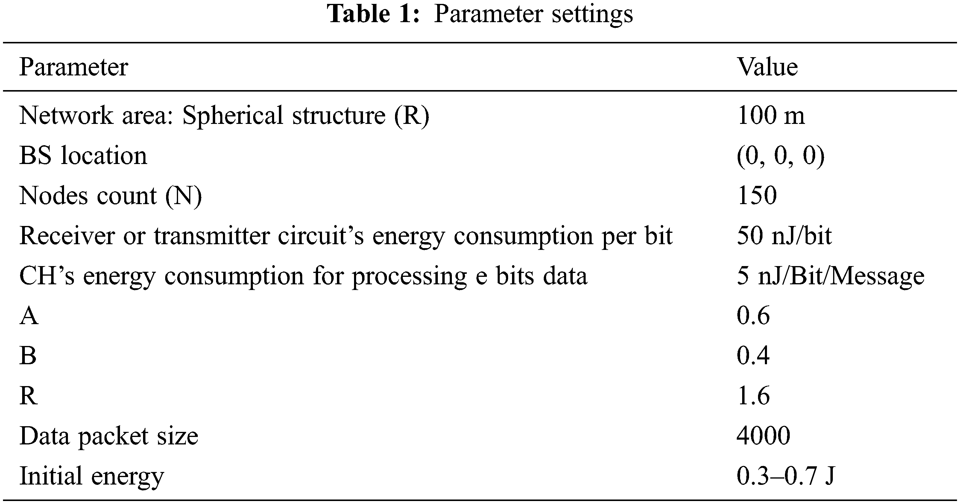
4.1 Energy Consumption Comparison
In this section, network energy consumption is discussed. It defines the WSN’s network residual energy, which is computed after every round. In a heterogeneous network, initial energy of node is defined with 0.3–0.7 J.
Techniques like Improved Dynamic Hierarchical Clustering (IDHC), Distributed Energy-Efficient Clustering (DEEC), Hybrid Energy Efficient Distributed (HEED) and Stable Election Protocol (SEP) are used making performance comparison. Residual energy comparison between available routing protocols like IDHC3D, DEEC3D, HEED3D, SEP3D and proposed ILDA-IDHC3D algorithm has saved energy value of 24%, 21%, 14%, 17%, and 28% is shown in Fig. 5. In network energy consumption balancing, better performance is exhibited by proposed protocol, when compared with other four protocols.
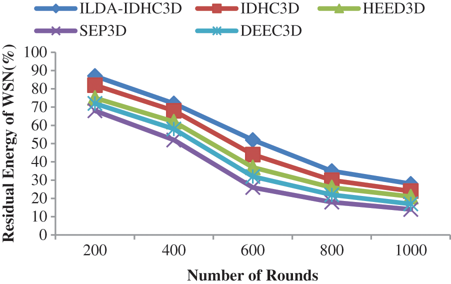
Figure 5: Residual energy vs. no. of rounds
4.2 Network Lifetime Comparison
At every round, alive nodes count defines the network lifetime. In this section, in heterogeneous networks, network lifetime is discussed and results of simulation are shown below.
In a heterogeneous network, SEP3D protocols are compared with HEED3D protocol in terms of alive nodes count and it is shown in Fig. 6. In 1000 rounds, 92 alive nodes are maintained by ILDA based IDHC (ILDA-IDHC3D) protocol, while 72 nodes are maintained by IDHC, 53 nodes by HEED3D, 35 nodes by DEEC3D and 24 nodes by SEP3D. More rounds of network communication can be carried by ILDA-IDHC3D protocol and heterogeneous network’s lifetime is increased.
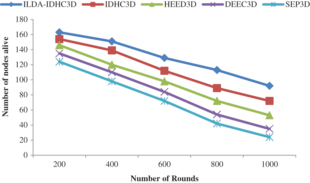
Figure 6: No. of alive nodes vs. no. of rounds
4.3 Network Throughput Comparison
In the network, packets count that is ultimately sent to BS defines the network throughput. In the form of packet, CH receives sensed information of every cluster member node. This sensed information is fused with sensed information of CH and at last, in packet form, this information is send to BS.
Network throughput performance metric comparison between existing protocols and proposed ILDA-IDHC3D protocol is shown in Fig. 7 using simulation results. Second highest network throughput is produced by IDHC3D protocol in heterogeneous networks as shown in Fig. 7. When compared with SEP3D, DEEC3D, HEED3D and IDHC3D around 57.07%, 28.78%, 39.89%, and 12.12% enhancement is shown by proposed ILDA-IDHC3D protocol.
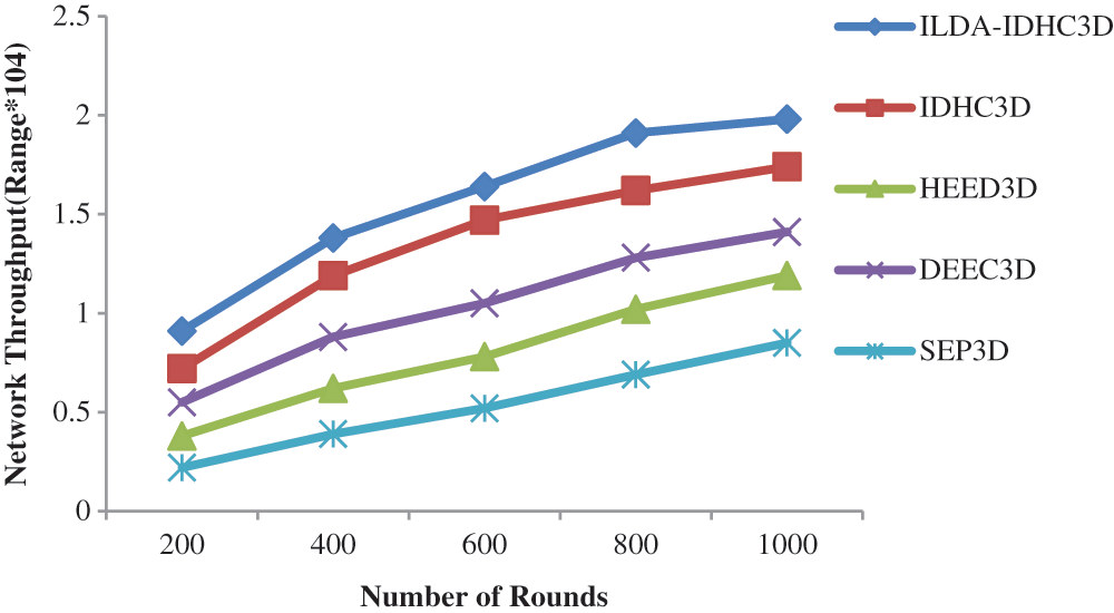
Figure 7: Network throughput vs. no. of rounds (0.3–0.7 J)
4.4 First Node Death Comparison
Performance of network can be measured using an important parameter called first node death round. Network will be pushed into unstable phase, after the death of first node and this indicates the decline in network performance. In heterogeneous networks, number of rounds before the death of first node comparison is shown in Fig. 8. Node’s energy is considered in IDHC3D and ILDA-IDHC3D protocol. In every round, node’s positional influence is considered for ensuring high energy and better position of CH node. Before the death of first node, double CH strategy is implemented. In addition, ILDA algorithm is used reducing dimensionality in the proposed work, which minimizes initial energy usage when compared with previous IDHC3D protocol.
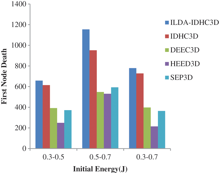
Figure 8: Round of the first node death vs. initial energy (heterogeneous network)
For hierarchical 3D WSNs, Incremental Linear Discriminant Analysis (ILDA) algorithm based effective dimensionality reduction model is proposed in this work. In order to reduce energy wastage in data or packet transmission, they are transmitted using ILDA algorithm. In intermediate nodes, transmitted bytes count is reduced by this technique, which enhances the lifetimeof the WSN. In the intermediate node, all of its incoming packets are aggregated into single packet using ILDA, so that, only a single packet will be send by intermediate node instead of relying on all incoming packets. Using this procedure, transmitted bits count € is minimized and it is termed as reduced bits (erd). This minimization is having noticeable effects on the nodes, which are in the base station’s vicinity. In a large cluster, cluster head loadis reduced using a Double Cluster Head (CH) approach. This is used for re-collecting CHs and updating the data transmission. With respect to the throughput, network residual energy, network lifetime and first node death, better performance is exhibited by proposed ILDA-IDHC3D routing protocol when compared to other protocols in heterogeneous network as shown in the results of simulation. When compared with conventional clustering protocols, the network lifespan is increased using cluster Head rotation policy in the proposed work. In future, the impact of relay nodes count and distribution on 3D WSN’s lifetime can be studied and explored. Moreover, the present WSN application could be extended to various 2D environment monitoring conditions.
Acknowledgement: We show gratitude to anonymous referees for their useful ideas.
Funding Statement: The authors received no specific funding for this study.
Conflicts of Interest: The authors declare that they have no conflicts of interest to report regarding the present study.
1. D. Kandris, C. Nakas, D. Vomvas and G. Koulouras, “Applications of wireless sensor networks: An up-to-date survey,” Applied System Innovation, vol. 3, no. 1, pp. 1–24, 2020. [Google Scholar]
2. S. Srivastava, M. Singh and S. Gupta, “Wireless sensor network: A survey,” in Int. Conf. on Automation and Computational Engineering (ICACE), Greater Noida, India, pp. 159–163, 2018. [Google Scholar]
3. D. Wohwe Sambo, B. O. Yenke, A. Försterand, P. Dayang, “Optimized clustering algorithms for large wireless sensor networks: A review,” Sensors, vol. 19, no. 2, pp. 1–27, 2019. [Google Scholar]
4. M. Noori and M. Ardakani, “Lifetime analysis of random event-driven clustered wireless sensor networks,” IEEE Transactions on Mobile Computing, vol. 10, no. 10, pp. 1448–1458, 2011. [Google Scholar]
5. S. Rani, J. Malhotra and R. Talwar, “Energy efficient chain based cooperative routing protocol for WSN,” Applied Soft Computing, vol. 35, no. 7, pp. 386–397, 2015. [Google Scholar]
6. M. Erol-Kantarci, H. T. Mouftah and S. Oktug, “A survey of architectures and localization techniques for underwater acoustic sensor networks,” IEEE Communications Surveys & Tutorials, vol. 13, no. 3, pp. 487–502, 2011. [Google Scholar]
7. M. Baghouri, A. Hajraoui and S. Chakkor, “Low energy adaptive clustering hierarchy for three-dimensional wireless sensor network,” in Institute of Natural Science and Engineering(INASE) in Recent Advances in Communications, Tetouan, Morocco, pp. 214–218, 2015. [Google Scholar]
8. J. Yan, M. Zhou and Z. Ding, “Recent advances in energy-efficient routing protocols for wireless sensor networks: A review,” IEEE Access, vol. 4, no. 10, pp. 5673–5686, 2016. [Google Scholar]
9. P. K. Batra and K. Kant, “LEACH-MAC: A new cluster head selection algorithm for wireless sensor networks,” Wireless Networks, vol. 22, no. 1, pp. 49–60, 2016. [Google Scholar]
10. S. M. Bozorgiand A. M. Bidgoli, “HEEC: A hybrid unequal energy efficient clustering for wireless sensor networks,” Wireless Networks, vol. 25, no. 8, pp. 4751–4772, 2018. [Google Scholar]
11. Hai, D.T. and Le Vinh, T., “Novel fuzzy clustering scheme for 3D wireless sensor networks,” Applied Soft Computing, vol. 54, pp. 141–149, 2017. [Google Scholar]
12. M. O. S. T. A. F. A. Baghouri, A. B. D. E. R. R. A. H. M. A. N. E. Hajraoui and S. A. A. D. Chakkor, “Stable election protocol for three dimensional clustered heterogeneous wireless sensor network,” WSEAS Transactions on Communications, vol. 16, pp. 298–305, 2017. [Google Scholar]
13. S. Vançin and E. Erdem, “Threshold balanced sampled DEEC model for heterogeneous wireless sensor networks,” Wireless Communications and Mobile Computing, vol. 2018, no. 11, pp. 1–12, 2018. [Google Scholar]
14. S. M. Hosen, G. H. Cho and I. H. Ra, “An eccentricity baseddata routing protocol with uniform node distribution in 3D WSN,” Sensors, vol. 17, no. 9, pp. 1–19, 2017. [Google Scholar]
15. D. T. Hai and T. Le Vinh, “Novel fuzzy clustering scheme for 3D wireless sensor network,” Applied Soft Computing, vol. 54, no. 5, pp. 141–149, 2017. [Google Scholar]
16. D. T. Tam, N. T. D. T. Hai, L. H. Son and L. T. Vinh, “Improving lifetime and network connections of 3D wireless sensor networks based on fuzzy clustering and particle swarm optimization,” Wireless Networks, vol. 24, no. 5, pp. 1477–1490, 2018. [Google Scholar]
17. Y. Jaradat, M. Masoud and I. Jannoud, “A mathematical framework of optimal number of clusters in 3D noise-prone WSN environment,” IEEE Sensors Journal, vol. 19, no. 6, pp. 2378–2388, 2019. [Google Scholar]
18. S. Balaji, E. G. Julie and Y. H. Robinson, “Development of fuzzy based energy efficient cluster routing protocol to increase the lifetime of wireless sensor networks,” Mobile Networks and Applications, vol. 24, no. 2, pp. 394–406, 2019. [Google Scholar]
19. J. G. Lee, S. Chim and H. H. Park, “Energy-efficient cluster-head selection for wireless sensor networks using sampling-based spider monkey optimization,” Sensors, vol. 19, no. 23, pp. 1–18, 2019. [Google Scholar]
20. J. Wang, Y. Gao, W. Liu, A. K. Sangaiah and H. J. Kim, “An improved routing schema with special clustering using PSO algorithm for heterogeneous wireless sensor network,” Sensors, vol. 19, no. 3, pp. 1–17, 2019. [Google Scholar]
21. Z. Zhao, D. Shi, G. Hui and X. Zhang, “An energy-optimization clustering routing protocol based on dynamic hierarchical clustering in 3D WSNs,” IEEE Access, vol. 7, no. 7, pp. 80159–80173, 2017. [Google Scholar]
22. F. Liu and Y. Chang, “An energy aware adaptive kernel density estimation approach to unequal clustering in wireless sensor networks,” IEEE Access, vol. 7, no. 4, pp. 40569–40580, 2019. [Google Scholar]
23. M. A. Rassam, A. Zainal and M. A. Maarof, “An adaptive and efficient dimension reduction model for multivariate wireless sensor networks applications,” Applied Soft Computing, vol. 13, no. 4, pp. 1978–1996, 2013. [Google Scholar]
24. A. Rooshenas, H. R. Rabiee, A. Movaghar and M. Y. Naderi, “Reducing the data transmission in wireless sensor networks using the principal component analysis,” in Sixth Int. Conf. on Intelligent Sensors, Sensor Networks and Information Proc., Brisbane, QLD, Australia, pp. 133–138, 2010. [Google Scholar]
25. W. Fang, W. Zhang, W. Chen, J. Liu, Y. Ni et al., “MSCR: Multidimensional secure clustered routing scheme in hierarchical wireless sensor networks,” EURASIP Journal on Wireless Communications and Networking, vol. 2021, no. 1, pp. 1–20, 2021. [Google Scholar]
26. X. Song, W. Sun and Q. Zhang,“A dynamic hierarchical clustering data gathering algorithm based on multiple criteriadecision making for 3d underwater sensor networks,” Complexity, vol. 2020, no. 8835103, pp. 1–14, 2020. [Google Scholar]
27. Z. Ullah, L. Mostarda, R. Gagliardi, D. Cacciagranoand F. Corradini, “A comparison of heed based clustering algorithms--Introducing ER-hEED,” in IEEE 30th Int. Conf. on Advanced Information Networking and Applications (AINA), Crans-Montana, Switzerland, pp. 339–345, 2016. [Google Scholar]
28. D. Chu, L. Z. Liao, M. K. P. Ng and X. Wang, “Incremental linear discriminant analysis: A fast algorithm and comparisons,” IEEE Transactions on Neural Networks and Learning Systems, vol. 26, no. 11, pp. 2716–2735, 2015. [Google Scholar]
 | This work is licensed under a Creative Commons Attribution 4.0 International License, which permits unrestricted use, distribution, and reproduction in any medium, provided the original work is properly cited. |