Computer Systems Science & Engineering DOI:10.32604/csse.2022.023109
Article

An Efficient Video Inpainting Approach Using Deep Belief Network

M. Nuthal Srinivasan1,* and M. Chinnadurai2

1Department of Electronics and Communication Engineering, E.G.S. Pillay Engineering College, Nagapattinam, 611002, Tamilnadu, India
2Department of Computer Science and Engineering, E.G.S. Pillay Engineering College, Nagapattinam, 611002, Tamilnadu, India
*Corresponding Author: M. Nuthal Srinivasan. Email: nuthalphd@gmail.com
Received: 28 August 2021; Accepted: 09 October 2021

Abstract: The video inpainting process helps in several video editing and restoration processes like unwanted object removal, scratch or damage rebuilding, and retargeting. It intends to fill spatio-temporal holes with reasonable content in the video. Inspite of the recent advancements of deep learning for image inpainting, it is challenging to outspread the techniques into the videos owing to the extra time dimensions. In this view, this paper presents an efficient video inpainting approach using beetle antenna search with deep belief network (VIA-BASDBN). The proposed VIA-BASDBN technique initially converts the videos into a set of frames and they are again split into a region of 5*5 blocks. In addition, the VIA-BASDBN technique involves the design of optimal DBN model, which receives input features from Local Binary Patterns (LBP) to categorize the blocks into smooth or structured regions. Furthermore, the weight vectors of the DBN model are optimally chosen by the use of BAS technique. Finally, the inpainting of the smooth and structured regions takes place using the mean and patch matching approaches respectively. The patch matching process depends upon the minimal Euclidean distance among the extracted SIFT features of the actual and references patches. In order to examine the effective outcome of the VIA-BASDBN technique, a series of simulations take place and the results denoted the promising performance.

Keywords: Video inpainting; deep learning; video restoration; beetle antenna search; deep belief network; patch matching; feature extraction

1  Introduction

Digital inpainting is widely employed in different applications such as object removal/image resolution and improvement restoration of images. The primary objective of digital inpainting is to complete the areas/regions by lacking information that has been vanished/lost intentionally. The inpainting model was stimulated by the artist utilizing their individual capabilities and acquaintance for reconstructing/fixing the damage which appeared in sculptures/paintings. Currently, the ability of digitalizing different kinds of visual data creates the requirement for methods which repair digital damages, as made with painting [1]. Furthermore, in communication, audio/video applications, it is necessary to retrieve the signals which get corrupted by narrowband intrusions such as electric hum [2]. The intervention could be determined sparsely in frequency domain (natural form). Video inpainting is an approach for filling the lost gaps/regions, retrieve object in a video. Removing unwanted objects in the video could generate lost regions [3]. The aim is to fill the lost regions hence the outcomes are convincing visually in space and time. Video inpainting could assist many restoration and video editing processes like scratch or damage restoration, retargeting, and unwanted removal of objects. Most importantly, and excepting its traditional demand, video inpainting could be employed with Augmented Reality (AR) for great visual experiences; Eliminating present item provides greater opportunity beforehand overlaying novel elements in a scene [4]. Hence, as a Diminished Reality (DR) technique, it opens up novel opportunities to be paired with novel deep learning or realtime based AR technology. Furthermore, there are many semi-online streaming scenarios like visual privacy filtering and automatic content filtering. Only a smaller wait would results in significant latency, therefore make the speed themselves a significant challenge.

In spite of considerable advances on DL based inpainting of an individual image, still it is stimulating to expand this method to video domain because of the extra time dimensions. The complications that come from difficult motion and higher requirements on temporal consistency make video inpainting a complex challenge [5]. A direct approach for performing video inpainting is to employ image inpainting on all frames separately. But, this ignores motions regularity come from the video dynamics, and hence it is unable to estimate the nontrivial appearance change in image space over time [6]. Furthermore, this system inevitably brings temporal inconsistency and cause serious flickering artifact. In order to tackle the temporal consistency, various approaches were introduced for filling the lost motion field; with a greedy election of local spatio and temporal patches, for each iterative optimization/frame diffusion based method [7]. But, the initial 2 method treats flow assessment to be self-governing of color assessment and lastly based on time consuming optimization.

This paper presents an efficient video inpainting approach using beetle antenna search with deep belief network (VIA-BASDBN). The proposed VIA-BASDBN technique initially converts the videos into a set of frames and they are again split into a region of 5*5 blocks. Followed by, the VIA-BASDBN technique involves the design of optimal DBN model, which receives input features from Local Binary Patterns (LBP) for the classification of blocks into smooth or structured regions. Moreover, the weight vectors of the DBN model are optimally chosen by the use of BAS technique. At last, the inpainting of the smooth and structured regions takes place using the mean and patch matching approaches respectively. For examining the superior performance of the VIA-BASDBN technique, a set of experimental analyses is carried out.

2  Literature Review

Patil et al. [8] proposed a novel inpainting method which depends on MS modeling, in which the original images are precisely attained by inpainting procedure in the masked image. Now, DWT method is employed to process is the digital images. Furthermore, to discover an optimum filter coefficient from DWT, a renowned optimization method called DA is employed. Furthermore, the smoothing of images is processed by regenerating kernel Hilbert smoothing models. Kim et al. [9] proposed a new DNN framework for faster video inpainting. Based on encoder-decoder models, this method is developed for collecting and refining data from neighboring frames and still synthesizes unknown regions. Simultaneously, the output is forced to be temporally reliable with a temporal memory and recurrent feedback model. Tudavekar et al. [10] proposed a new 2 phase architecture. Initially, subbands of wavelets of lower resolution images are attained by the dual tree complex WT. auto-regression and Criminisi algorithms are later employed to this sub-band for inpainting the lost region. The FL based histogram equalization is employed for additionally enhancing the image by maintaining the brightness of an image and enhance the local contrast. Next, the images are improved by a super resolution method. The procedure of inpainting, down-sampling and consequently improving the videos by the super resolution techniques reduce the video inpainting time. To decrease the computation complexity of image inpainting, an enhanced Criminisi algorithm is presented in [11] on the basis of BBO model. Based on characteristics of Criminisi, the novel methods use the mutation and migration of BBO model for searching optimal matching blocks and conquer the shortcoming of Criminisi algorithms through searching optimal matching blocks in the unbroken region in an image.

Janardhana Rao et al. [12] aimed to improve new DL concepts for handling video inpainting. In the first step, motion tracing is carried out, i.e., the procedure of defining motion vector which describes the conversion from neighboring frame in a sequence video. Furthermore, the patches/regions of all the frames are classified by an enhanced RNN, where the regions are divided into a structure and smooth regions. This can be implemented by the texture features named grey level co-occurrence matrix. Now, the hybridization of 2 Meta heuristic approaches such as CS and MVO algorithms named CSMVO is employed for optimizing the patch matching and RNN model. Ding et al. [13] proposed a novel forensic refinement architecture for localizing the deep in painted region with the consideration of spatial temporal viewpoints. Initially, designed spatiotemporal convolutions for suppressing redundancy to highlight deep inpainting traces. Next, a detection model is made by 2 up sampling layers and 4 concatenated ResNet blocks, for achieving a rough localization map. Lastly, an adapted U-net based refinement modules are presented to the pixelwise location mapping. Zeng et al. [14] proposed to learn a joint STTN to video inpainting. Particularly, fill lost region in each input frame through self-attention, also proposed to enhance STTN through a spatial temporal adversarial loss. In order to exhibit the dominance of the presented approach, they performed qualitative and quantitative assessments with the aid of standard stationary mask.

Li et al. [15] presented a new context aggregation network for effectively exploiting short-term and long term frame data to video inpainting. In encoding phase, they proposed boundary aware short-term context aggregation, that align and aggregate, from neighboring frame, local region is related closely to the edge context of lost region to the targeting frames (represents the present input frames under inpainting.). Further, proposed a dynamic long term context aggregation for widely refining the feature map made in the encoding phase. Hirohashi et al. [16] proposed to adapt a newly presented video inpainting methods which are capable of restoring higher fidelity images in real time. It estimates optical flows with a CNN also utilizes them for matching occluded regions in the present frames to unconcluded regions in prior frames, restore the previous. Even though the direct applications doesn't lead to acceptable result because of the peculiarity of the SMC video, they demonstrate that 2 improvement makes it promising to attain better result. Zou et al. [17] proposed the Progressive Temporal Feature Alignment Network’, that gradually enrich feature extracted from the present frames using the feature wrapped from neighboring frame with optical flows. This approach corrects the spatial misalignment in the temporal feature propagation phase, highly improves temporal consistency and visual quality of the inpainting video. Wu et al. [18] proposed a novel DAPC-Net model that utilizes temporal redundancy data amongst video sequences. Especially, create a DANet mode to align reference frames at the feature level. Afterward, alignment devised a PCNet for completing lost region of the targeting frames.

3  The Proposed Model

In this study, a novel VIA-BASDBN technique is derived for effective video inpainting process. Initially, the input videos are converted into frames and down-sampling process is carried out. Besides, the LBP technique extracts the features and fed into the ODBN model for the classification of regions into smooth/structure. Finally, the video inpainting of the smooth and structured regions is carried out by mean and patch matching approaches. Fig. 1 illustrates the overall block diagram of VIA-BASDBN model.

Figure 1: Block diagram of VIA-BASDBN model

3.1 Frame Conversion and Down-Sampling

Primarily, the frame extraction process from the input video is carried out and the frames are down sampled to a factor of 2 to obtain low resolution images. The inpainting of the low-resolution image is not affected by noise and thereby the computation cost becomes low. When the low-resolution images are produced, the current image gets subtracted from the previous one. If the residual value results in 0 or less than predefined pixel value, it can be concluded that the inpainting process is not needed. Otherwise, the inpainting process takes place using the VIA-BASDBN technique.

3.2 Design of Optimal DBN Model for Smooth/Structure Region Classification

Once the videos are converted into a set of frames, every region of the frame is again split into 5*5 blocks which are then classified by ODBN model into smooth or structured regions. The ODBN model receives the features as input from the LBO model. At the time of training the DBN model, it retains the target as smooth or structure depending upon the standard deviation (SD) of the particular block. When the SD becomes lower than 5, the target is treated as smooth one. Otherwise, it is considered as the structure region, as given below.

type={structureifSD>5smoothotherwise (1)

In order to improve the performance of the DBN model, the weight vectors of the DBN model are optimally tuned using the BAS.

3.2.1 LBP Model

The LBP features are derived to provide input to the ODBN model for the classification of regions into smooth and structured regions. It offers a descriptor for the images by the use of grayscale values for every pixel. Traditionally, every pixel considers its neighboring eight pixels and creates a block of 3 × 3 pixels. Followed by, the relation with the intermediate pixel with other 8 neighboring pixels are determined [19]. When the grayscale value exceeds the intermediate pixel, it gets substituted by 1; else it becomes 0. The resultant binary pattern is transformed to a decimal number. The LBP operator can be represented as follows:

LBP(xc′yc)=∑p∈P⁡2p∗q(ip−ic), (2)

where P denotes the pattern describing the pixel located nearer to the intermediate pixel, ic and i, denotes the grayscale value of the intermediate and p-th neighbor, and q(z) is a quantization function represented by:

q(z)={1, z≥00, otherwise (3)

It is noticed that the neighboring pixel count and the radius are the variables which be altered or remain same.

3.2.2 DBN Based Classification Model

The DBN model receives the LBP features as input and categorizes the regions into smooth and structured ones. RBM consists of 2 two layers i.e., stochastic network: the visible layer and hidden layer. The collected data is denoted as visible layer, where the hidden layers attempt to learn features from visible layers focuses for demonstrating the probabilistic data distribution. The network is called restricted since the layer neuron comprises connection toward the neuron in other layers. Connections between layers are symmetric and bidirectional, allowing data transmission. Fig. 2 displays the structure of RBM, where neurons count is represented as m within visible layers (v1, …, vm), within hidden layers (h1, …, hn), n represent the amount of neurons, bias vector is represented as a & b and weight matrix is represented as w. RBM employ hidden layers variable for designing the probabilistic distribution on visible attribute. The initial layer is performed using visible unit and based on the observation element for each input pattern feature, single visible units are performed. The initial layer is performed using visible units and based on observation elements i.e., single visible units for each input pattern feature. The dependency of hidden unit models amongst the observation elements i.e., dependencies amongst features. Probability distribution on variable h & v is defined by an entropy function that is called as Energy based model.

Figure 2: DBN structure

Using aforementioned equation, the functions are determined in extensive and vectorial formats as:

E(v,h)=−hTWv−aTv−bTh (4)

E(v,h)=−∑i,j=1m,n⁡vihjwij−∑i=1m⁡aivi−∑i=1n⁡bjhj (5)

For each neuron pair in network, it is possible to assign probabilities through entropy function, in visible and hidden layers, provide a probabilistic distribution.

p(v,h)=e−E(v,h)∑v,h⁡e−E(v,h) (6)

The vector probabilities from v as visible layers are provided as overall vector probabilities beyond the hidden layers

p(v)=∑h⁡e−E(v,h)∑v,h⁡e−E(v,h) (7)

Since the RBM doesn't comprise a connection between nearby neurons of related layers, the action is autonomous. It offers the limited probability calculation as

p(h|v)=∏j⁡p(hj|v) (8)

p(h|v)=∏i⁡p(vi|h) (9)

The initial RBM version is constructed for resolving problems in binary data. Using the accurate distribution (8) & (9) is generated by

p(hj=1|v)=sigm(bj+∑i=1m⁡viwij) (10)

p(vj=1|h)=sigm(aj+∑j=1n⁡hiwij) (11)

Here, sigmoid function represents the sigm(x). The problem solving potentials are limited with RBM for binary data. The RBM forms are applied that enable subsequent data for enhancing the accuracy problems. Gauss types RBM is the popular type of RBM. The visible layer probable distribution in this RBM is adapted toward Gaussian distribution. This variance is called as Gaussian–Bernoulli RBM. The Gaussian–Bernoulli RBM probability distribution is given below

p(hj=1|v)=sigm(bj+1σ2∑i=1m⁡viwij) (12)

p(vj=1|h)=N(ai+∑j=1n⁡hjwij,σ2) (13)

The training RBM includes decreasing negative log-probability given as follows

Δwij=e∂log⁡p(V)∂wij=evihjm (14)

Learning rate is represented as e, 〈▪〉d & 〈▪〉m is used for denoting the model and desirable data rate respectively. For binary data, the expectation is drawn from Eqs (10) & (11) where, for constant data, the (14) & (15) gives expectation. The DBN has been generative graphical method which is a class of DNNs. Once the CD is established, Hinton [20] projected to stack trained RBM from the greedy approach for creating the called DBN. This is deep layer network with all layers being an RBM network stacked together for construction of a DBN.

In DBN structure, all 2 sequential hidden layer procedures an RBM. An input layer of current RBM is usually the resultant layer of preceding RBM. The DBN has been graphical method which contains deep hierarchical representation of trained data. The joint probability distribution of visible vector v and l hidden layer (hk(k = 1, 2, …, l), h0 = v) is demonstrated utilizing the subsequent equation:

P(hh2,..,.,hl|V)=P(hl|hl−1)P(hl−1|hl−2)…P(h|v)P(h1,h2,…,h1|v)=P(hl|hl−1)P(hl−1|hl−2)…P(h1|v)

=∏k=1l⁡P(hk|hk−1) (15)

The probabilities of bottom-up inference in the visible layer v to hidden layer hk, is determined as:

P(hk|hk−1)=σ(bjk+∑j=1m⁡wijkhjk−1), (16)

where bk represents the bias to the layer kth

Comparison, the top-down inference from the symmetric version of bottom-up inference that is expressed as [21]:

P(hk−1|hk)=σ(ajk−1+∑j=1m⁡wijk−1hjk), (17)

where ak−1 signifies the bias to the layer (k − 1)th

The trained of DBN is separated as to 2 phases: pre-training and fine-tuning utilizing BP. Pre- training subsequently fine-tuning has been great mechanism to train as DBN.

3.2.3 Optimal DBN Using BAS Technique

At the time of training the DBN model, the weights of the DBN are optimally selected by the use of BAS and thereby improves the classification performance. The major aim of the ODBN model is to minimize the error between the estimated and actual outcome, as defined below.

Obj=argmin{Wg}⁡{err}anderr=CLE−CLO

where CLE is the estimated output of the DBN model and CLO denotes the original target output. BAS algorithm is one of the smart optimization methods which simulate beetles forage behaviors. Once a beetle's forage, it would employ its right and left antennae for sensing the odor intensity of food. When the odor intensity obtained through the left antennae's are larger, it would fly to the left through the stronger odor intensity; or else, it would fly to the right. The modelling procedure of BAS algorithms are given in the following:

b→= rands(Dim,1)‖rands(Dim,1)‖ (18)

Whereas Dim represents the spatial dimension. The space coordinate of the beetles right and left sides and its antennae is made by

{xrt=xt+d0∗b→/2xlt=xt−d0∗b→/2 (19)

Amongst other, xt represent the location of beetles’ antennae in t-th iteration, xrt represent the location of beetles’ right antennae in t-th iteration, xlt represent the location of beetles left antennae in t-th iteration, and d0 represent the beetles’ 2 locations [22]. Based on the elected FF, the corresponding fitness value of the right and left antennae are estimated, and the beetles move toward the antennae using a smaller fitness number. The position of beetles are iteratively upgraded by

xt+1=xt+δt∗b→∗sign(f(xrt)−f(xlt)) (20)

Amongst other, δt denotes the step factor, sign indicates a sign function, and eta represents the variable step factor, that is generally 0.95.

3.3 Video Inpainting Process

At this stage, the video inpainting process takes place in two ways. When the classified region is smooth, the inpainting process takes place by taking the mean value of pixels related to the unmasked region of the patch. On the other hand, when the classification region is structured, the patch matching process takes place using SIFT and Euclidean distance.

3.3.1 Inpainting of Smooth Regions

In order to accomplish inpainting of every individual frame in the video, it is partitioned into a set of 28 × 28 blocks. Then, the masked regions are in black whose pixel is signified as ‘0’. They are given into the trained ODBN model to determine the particular block as smooth or structure. If no uniform texture data exist in the patch area, then it is treated as smooth. Then, the inpainting of smooth regions is carried out by placing the pixels of all blocks among the patches using the mean or average pixel values relevant to the unmasked region of the patch. For instance, in case of 28 × 28 patch, consider the unmasked pixel count as Nu and the pixel is defined by INue where ue  =  1, 2, …, Nu. The mean of the pixel can be represented by

INuenew=1Nu∑ue−1Nu⁡INue (21)

Therefore, the ueth pixel INue has changed with novel mean pixel.

3.3.2 Inpainting of Structure Regions

At the time of inpainting the structure regions, the frames are split into 28 × 28 blocks. Furthermore, the SIFT features are derived for the respective blocks. It is an effective technique which is invariant to the modifications in the illumination and permits changes in the existence of occlusions, clutter, and noise. It is strong o affine the transformation, cluttering, and occlusion. When the SIFT features are determined for a specific block, it is needed to calculate the SIFT features of the residual patches in the image. Therefore, the patches get substituted with the patch holding lower Euclidean distance. This process gets iterated for every residual structure region that exists in the frame.

4  Performance Validation

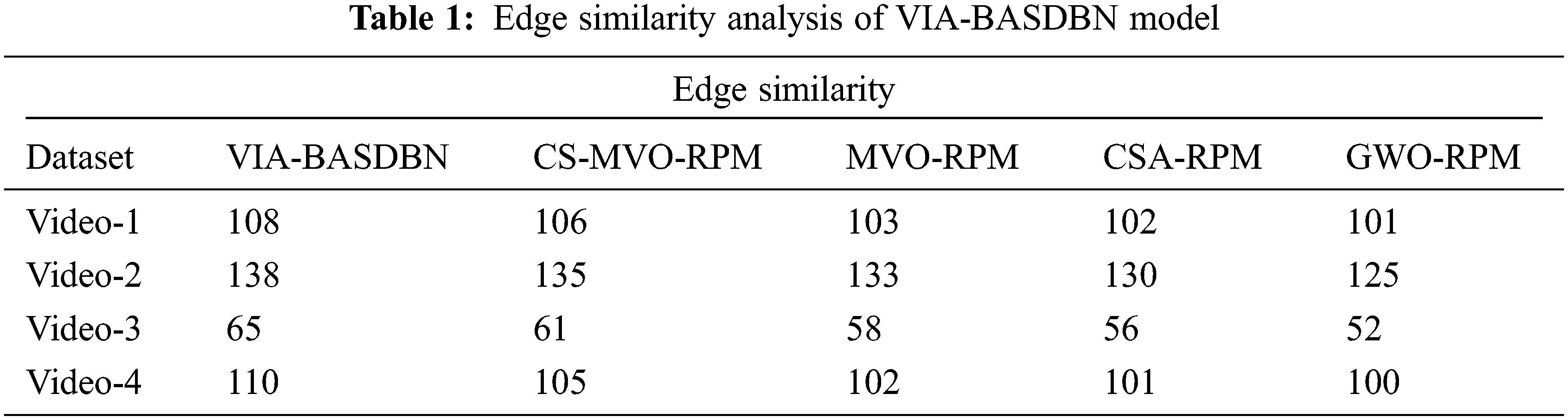
It will speed up the review and typesetting process. This section investigates the performance of the VIA-BASDBN technique using MATLAB tool against four test videos. Videos 1 and 2 are gathered from [23] which consists of 104 frames. In addition, videos 3 and 4 are taken from [24], comprises 15 frames. Fig. 3 shows the sample videos sequences of 1 and 2. Similarly, Fig. 4 depicts the sample videos of 3 and 4. Tab. 1 and Fig. 5 offer the edge similarity analysis of the VIA-BASDBN technique with existing methods under four test videos. The results portrayed that the VIA-BASDBN technique has accomplished effectual outcomes over the existing techniques with the higher edge similarity. For instance, on the test video-1, the VIA-BASDBN technique has accomplished an increased edge similarity of 108 whereas the CS-MVO-RPM, MVO-RPM, CSA-RPM, and GWO-RPM techniques have attained a reduced edge similarity of 106, 103, 102, and 101 respectively. Moreover, on the test video-3, the VIA-BASDBN technique has resulted in a higher edge similarity of 138 whereas the CS-MVO-RPM, MVO-RPM, CSA-RPM, and GWO-RPM techniques have attained a lower edge similarity of 135, 133, 130, and 125 respectively. Furthermore, on the test video-4, the VIA-BASDBN technique has provided an improved edge similarity of 110 whereas the CS-MVO-RPM, MVO-RPM, CSA-RPM, and GWO-RPM techniques have exhibited a decreased edge similarity of 105, 102, 101, and 100 respectively.

Figure 3: Sample sequences (video 1 and video 2)

Figure 4: Sample sequences (video 3 and video 4)

Figure 5: Edge similarity analysis of VIA-BASDBN model

A comprehensive MSE analysis of the VIA-BASDBN technique with existing methods takes place in Tab. 2 and Fig. 6. The results demonstrated that the VIA-BASDBN technique has resulted in an effective outcome with the least MSE. For instance, under test video-1, the VIA-BASDBN technique has demonstrated a lower MSE of 57.35 whereas the CS-MVO-RPM, MVO-RPM, CSA-RPM, and GWO-RPM techniques have offered a higher MSE of 58.85, 59.04, 64.24, and 64.43 respectively.

Figure 6: MSE analysis of VIA-BASDBN model

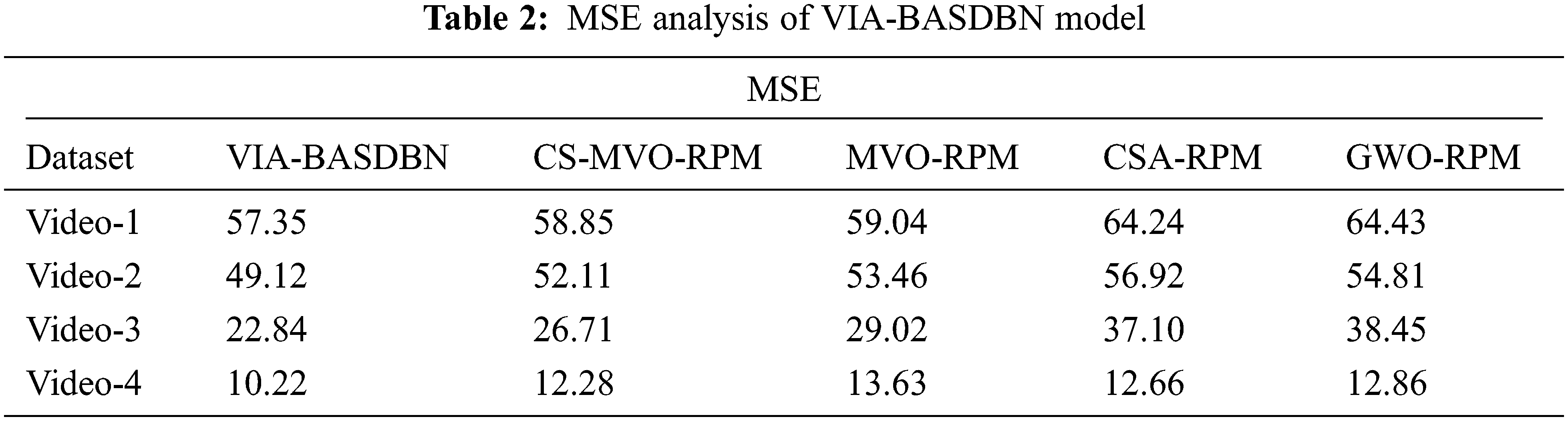
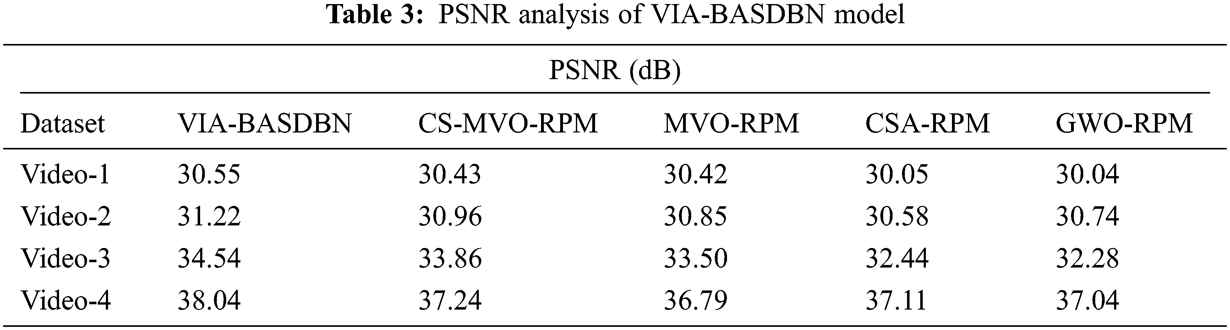
Concurrently, under test video-3, the VIA-BASDBN manner has showcased a minimal MSE of 22.84 whereas the CS-MVO-RPM, MVO-RPM, CSA-RPM, and GWO-RPM algorithms have obtainable a superior MSE of 26.71, 29.02, 37.10, and 38.45 correspondingly. Eventually, under test video-4, the VIA-BASDBN method has outperformed a reduced MSE of 10.22 whereas the CS-MVO-RPM, MVO-RPM, CSA-RPM, and GWO-RPM methodologies have accessible an increased MSE of 12.28, 13.63, 12.66, and 12.86 correspondingly. Tab. 3 and Fig. 7 provide the PSNR analysis of the VIA-BASDBN manner with existing techniques under four test videos. The outcomes exhibited that the VIA-BASDBN technique has accomplished effective outcomes over the existing manners with maximum PSNR. For instance, on the test video-1, the VIA-BASDBN algorithm has accomplished an enhanced PSNR of 30.55 dB whereas the CS-MVO-RPM, MVO-RPM, CSA-RPM, and GWO-RPM methods have attained a reduced PSNR of 30.43, 30.42, 30.05, and 30.04 dB correspondingly. Furthermore, on the test video-3, the VIA-BASDBN approach has resulted in a higher PSNR of 34.54 dB whereas the CS-MVO-RPM, MVO-RPM, CSA-RPM, and GWO-RPM techniques have gained a minimum PSNR of 33.86, 33.50, 32.44, and 32.28 dB correspondingly. Additionally, on the test video-4, the VIA-BASDBN manner has offered a maximum PSNR of 38.04 dB whereas the CS-MVO-RPM, MVO-RPM, CSA-RPM, and GWO-RPM methods have outperformed a reduced PSNR of 37.24, 36.79, 37.11, and 37.04 dB correspondingly.

Figure 7: PSNR analysis of VIA-BASDBN mode

Tab. 4 and Fig. 8 offer the SNR analysis of the VIA-BASDBN approach with existing techniques under four test videos. The results portrayed that the VIA-BASDBN technique has accomplished effective results over the existing techniques with the higher SNR. For instance, on the test video-1, the VIA-BASDBN technique has accomplished an increased SNR of 15.31 dB whereas the CS-MVO-RPM, MVO-RPM, CSA-RPM, and GWO-RPM techniques have attained a lower SNR of 14.96, 14.87, 13.49, and 13.45dB correspondingly. Followed by, on the test video-3, the VIA-BASDBN algorithm has resulted in a higher SNR of 15.94 dB whereas the CS-MVO-RPM, MVO-RPM, CSA-RPM, and GWO-RPM manners have obtained a decreased SNR of 15.73, 14.95, 13.76, and 13.57 dB respectively. Finally, on the test video-4, the VIA-BASDBN approach has provided a higher SNR of 14.79 dB whereas the CS-MVO-RPM, MVO-RPM, CSA-RPM, and GWO-RPM methodologies have showcased a decreased SNR of 14.49, 14.35, 14.12, and 14.03 dB correspondingly.

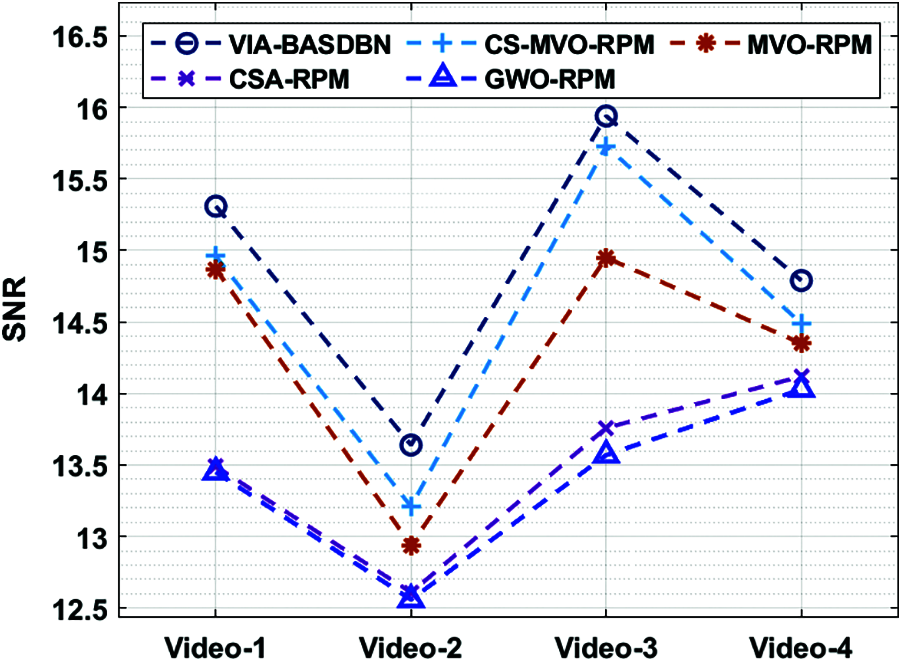
Figure 8: SNR analysis of VIA-BASDBN model

From the above mentioned tables and figures, it is apparent that the VIA-BASDBN technique has accomplished maximum video inpainting performance over the other recent techniques.

5  Conclusion

In this study, a novel VIA-BASDBN technique is derived for effective video inpainting process. Initially, the input videos are converted into frames and down-sampling process is carried out. Besides, the LBP technique extracts the features and fed into the ODBN model for the classification of regions into smooth/structure. Finally, the video inpainting of the smooth and structured regions is carried out by mean and patch matching approaches. For examining the superior performance of the VIA-BASDBN technique, a set of experimental analyses is carried out. The simulation results pointed out the supremacy of the VIA-BASDBN technique over the recent techniques interms of different aspects. Therefore, it can be employed as an effective tool for video inpainting. In future, recent DL architectures with bioinspired algorithms can be used for patch matching process to improve the overall efficiency of the VIA-BASDBN technique.

Funding Statement: The authors received no specific funding for this study.

Conflicts of Interest: The authors declare that they have no conflicts of interest to report regarding the present study.

References

 1.  U. A. Ignacio and C. R. Jung, “Block-based image inpainting in the wavelet domain,” The Visual Computer, vol. 23, no. 9–11, pp. 733–741, 2007. [Google Scholar]

 2.  H. Xue, S. Zhang and D. Cai, “Depth image inpainting: Improving low rank matrix completion with low gradient regularization,” IEEE Journals & Magazines, vol. 26, no. 9, pp. 4311–4320, 2017. [Google Scholar]

 3.  C. Ballester, M. Bertalmio, V. Caselles, G. Sapiro and J. Verdera, “Filling-in by joint interpolation of vector fields and gray levels,” IEEE Transactions on Image Processing, vol. 10, no. 8, pp. 1200–1211, 2001. [Google Scholar]

 4.  C. Barnes, E. Shechtman, A. Finkelstein and D. B. Goldman, “Patchmatch: A randomized correspondence algorithm for structural image editing,” ACM Transactions on Graphics (ToG), vol. 28, no. 3, pp. 1–24, 2009. [Google Scholar]

 5.  T. Shiratori, Y. Matsushita, X. Tang and S. B. Kang, “Video completion by motion field transfer,” in Proc. IEEE Computer Society Conf. on Computer Vision and Pattern Recognition (CVPR'06), New York, USA, vol. 1, pp. 411–418, 2006. [Google Scholar]

 6.  Y. Matsushita, E. Ofek, W. Ge, X. Tang and H. Y. Shum, “Full-frame video stabilization with motion inpainting,” IEEE Transactions on Pattern Analysis and Machine Intelligence, vol. 28, no. 7, pp. 1150–1163, 2006. [Google Scholar]

 7.  J. B. Huang, S. B. Kang, N. Ahuja and J. Kopf, “Temporally coherent completion of dynamic video,” ACM Transactions on Graphics (TOG), vol. 35, no. 6, pp. 196–212, 2016. [Google Scholar]

 8.  B. H. Patil and P. M. Patil, “Hybrid image inpainting using reproducing kernel hilbert space and dragonfly inspired wavelet transform,” International Journal of Nano and Biomaterials, vol. 8, no. 3–4, pp. 301–320, 2019. [Google Scholar]

 9.  D. Kim, S. Woo, J. Y. Lee and I. S. Kweon, “Deep video inpainting,” in Proc. IEEE/CVF Conf. on Computer Vision and Pattern Recognition, New Orleans, United States, pp. 5792–5801, 2019. [Google Scholar]

10. G. Tudavekar, S. R. Patil and S. S. Saraf, “Dual-tree complex wavelet transform and super-resolution based video inpainting application to object removal and error concealment,” CAAI Transactions on Intelligence Technology, vol. 5, no. 4, pp. 314–319, 2020. [Google Scholar]

11. W. Yao, X. Zhou, L. Zhang, M. Yang and S. Yan, “A biogeography-based optimization algorithm for criminisi algorithm,” in Proc. 4th Int. Conf. on Multimedia Systems and Signal Processing (ICMSSP 2019), Newyork, United States, pp. 25–30, 2019. [Google Scholar]

12. B. J. Rao, Y. Chakrapani and S. S. Kumar, “Hybridized cuckoo search with multi-verse optimization-based patch matching and deep learning concept for enhancing video inpainting,” The Computer Journal, vol. Preprint, pp. 1–24, 2021. [Google Scholar]

13. X. Ding, Y. Pan, K. Luo, Y. Huang, J. Ouyang et al., “Localization of deep video inpainting based on spatiotemporal convolution and refinement network,” in Proc. IEEE Int. Symp. on Circuits and Systems (ISCAS), Daegu, Korea, pp. 1–5, 2021. [Google Scholar]

14. Y. Zeng, J. Fu and H. Chao, “Learning joint spatial-temporal transformations for video inpainting,” in Proc. European Conf. on Computer Vision, Glasgow, UK, pp. 528–543, 2020. [Google Scholar]

15. A. Li, S. Zhao, X. Ma, M. Gong, J. Qi et al., “Short-term and long-term context aggregation network for video inpainting,” in Proc. European Conf. on Computer Vision, Glasgow, UK, pp. 728–743, 2020. [Google Scholar]

16. Y. Hirohashi, K. Narioka, M. Suganuma, X. Liu, Y. Tamatsu et al., “Removal of image obstacles for vehicle-mounted surrounding monitoring cameras by real-time video inpainting,” in Proc. IEEE/CVF Conf. on Computer Vision and Pattern Recognition, New Orleans, United States, pp. 214–215, 2020. [Google Scholar]

17. X. Zou, L. Yang, D. Liu and Y. J. Lee, “Progressive temporal feature alignment network for video inpainting,” in Proc. IEEE/CVF Conf. on Computer Vision and Pattern Recognition, New Orleans, United States, pp. 16448–16457, 2021. [Google Scholar]

18. Z. Wu, K. Zhang, H. Xuan, J. Ye and Y. Yan, “DAPC-Net: Deformable alignment and pyramid context completion networks for video inpainting,” IEEE Signal Processing Letters, vol. spl.28, pp. 1–22, 2021. [Google Scholar]

19. L. Nanni, E. D. Luca, M. L. Facin and G. Maguolo, “Deep learning and handcrafted features for virus image classification,” Journal of Imaging, vol. 6, no. 12, pp. 143–158, 2020. [Google Scholar]

20. G. E. Hinton, “Deep belief network,” Scholarpedia, vol. 4, no. 5, pp. 5947–5964, 2009. [Google Scholar]

21. P. Sokkhey and T. Okazaki, “Development and optimization of deep belief networks applied for academic performance prediction with larger datasets,” IEIE Transactions on Smart Processing & Computing, vol. 9, no. 4, pp. 298–311, 2020. [Google Scholar]

22. L. Zhou, K. Chen, H. Dong, S. Chi and Z. Chen, “An improved beetle swarm optimization algorithm for the intelligent navigation control of autonomous sailing robots,” IEEE Access, vol. 9, pp. 5296–5311, 2020. [Google Scholar]

23. A. Newson, A. Almansa, M. Fradet, Y. Gousseau and P. Perez, “Video inpainting of Complex scenes”, SIAM Journal of Imaging Sciences, vol. 20, pp. 1–27, 2019. [Google Scholar]

24. Y. L. Chang, Z. Y. Liu, K. Y. Lee and W. Hsu,“Learnable gated temporal shift module for deep video inpainting”, in proc. 30th British Machine Vision Conference, Cardiff, UK, pp. 1–20, 2019. [Google Scholar]

This work is licensed under a Creative Commons Attribution 4.0 International License, which permits unrestricted use, distribution, and reproduction in any medium, provided the original work is properly cited.