DOI:10.32604/csse.2022.023376
| Computer Systems Science & Engineering DOI:10.32604/csse.2022.023376 | |
| Article |
Kalman Filter and H∞ Filter Based Linear Quadratic Regulator for Furuta Pendulum
1Department of Electronics and Instrumentation Engineering, Government College of Technology, Coimbatore, Tamil Nadu, India
2Department of Electrical and Electronics Engineering, Anna University, Regional Campus, Coimbatore, Tamil Nadu, India
*Corresponding Author: N. Arulmozhi. Email: arulmozhimozhi609@gmail.com
Received: 06 September 2021; Accepted: 16 November 2021
Abstract: This paper deals with Furuta Pendulum (FP) or Rotary Inverted Pendulum (RIP), which is an under-actuated non-minimum unstable non-linear process. The process considered along with uncertainties which are unmodelled and analyses the performance of Linear Quadratic Regulator (LQR) with Kalman filter and H∞ filter as two filter configurations. The LQR is a technique for developing practical feedback, in addition the desired x shows the vector of desirable states and is used as the external input to the closed-loop system. The effectiveness of the two filters in FP or RIP are measured and contrasted with rise time, peak time, settling time and maximum peak overshoot for time domain performance. The filters are also tested with gain margin, phase margin, disk stability margins for frequency domain performance and worst case stability margins for performance due to uncertainties. The H-infinity filter reduces the estimate error to a minimum, making it resilient in the worst case than the standard Kalman filter. Further, when the β restriction value lowers, the H∞ filter becomes more robust. The worst case gain performance is also focused for the two filter configurations and tested where H∞ filter is found to outperform towards robust stability and performance. Also the switchover between the two filters is dependent upon a user-specified co-efficient that gives the flexibility in the design of non-linear systems. The non-linear process is tested for set point tracking, disturbance rejection, un-modelled noise dynamics and uncertainties, which records robust performance towards stability.
Keywords: Furuta pendulum; linear quadratic regulator; kalman filter; non-linear process; two filter configurations
The international federation of automatic control theory committee had formulated an array of bench mark control problems, in which the inverted pendulum is enlisted as highly unstable control problem due to its high non-linearity’s and lack of stability [1]. It finds practical applications in robot arms with cylindrical geometry, rotary cranes, segway, and goods carrying pendulous, earthquake resistant building designs and even in human walking and more essentially it serves as a prototype in the missile or rocket launcher dynamics with its center of gravity located behind the center of drag that causes aerodynamic instability.
The Rotary Inverted Pendulum (RIP) is characterized by non-linear dynamic equations that portraits the unstable equilibrium position of inverted pendulum with respect to the centre of gravity. It has a zero at right-half plane of s-plane the makes it a non-minimum phase system affecting the stability and robustness [2]. The RIP has two degrees of freedom viz., the rotor arm angle and pendulum angle but one actuator i.e., Direct Current (DC) motor is used to control both degrees of freedom. This categorizes the system to be an under actuated system and builds the complexity of the control problem to be challenging. The control problem is added with constraints imposed by physical dimensions such as mass and length of rotor arm and pendulum and the control voltage offered to DC motor to position the rotor and pendulum at desired location [3]. This makes the control problem challenging and attracts attention to attempt various control strategies.
The stabilization of planar pendulum is discussed in [4] when it switches between positive and negative feedbacks, considering the upright position of the pendulum as saddle point. The input-output linearization, energy control, and singular perturbation theory and prints the time-domain based result i.e., step response of pendulum angle and cart position of a planar pendulum is discussed in [5]. The properties of swing-up strategies of inverted pendulum and the swing-up property mainly influenced by acceleration of pivot and that of gravity are investigated in [6]. It also gives a hint on robustness of minimum time swing in terms of energy overshoot with control action response. Furuta Pendulum (FP) dynamics using a lagrangian formulation and an iterative Newton-Euler formulation and the result using the time response of single rotary inverted pendulum are presented in [7].
A periodic controller is employed [8] for a planar pendulum and the stability regions are tested after implementing a controller with root locus. A Takagi-Sugeno approach in designing a fuzzy controller for balancing the planar type inverted pendulum with much computational effort is discussed in [9] and the results with step response of associated parameters are also given. It establishes fast and safe swing up stabilization of RIP using Linear Quadratic Regulator (LQR) with step response along with Disturbance Rejection (DR) in [10]. An adaptive controller is designed in [11] for stabilizing a RIP in is upright position. The time response of cart position, pendulum angle and the corresponding control action by designing a PI-state feedback pole placement technique is displayed in [12]. A comparison of step responses of cart positions, pendulum angle by designing the Proportional-Integral-Derivative (PID) and LQR control methods for planar pendulum with and without disturbance input are discussed in [13].
Linear Quadratic Gaussian (LQG) and LQR with Kalman filter for an aircraft control system and print the impulse and step response of pitch, roll and yaw are explained in [14]. A control method based on feedback linearization for the FP is discussed in [15] which, also compares the time response analysis with PID controller. The effect of adaptive feedback using the estimates of matrix A that concerns to the stabilization of a double-inverted pendulum is discussed in [16] without exact knowledge of dynamic equations and in the presence of external bounded perturbations. Fractional order controller for stabilization of rotational inverted pendulum and D-decomposition technique for identifying stability regions in the controller parameter space are employed in [17]. It shows the result with respect to impulse response and not step response.
An aid in choosing controller gains for regulation of FP in view of student lab formation is discussed in [18]. The two forms of LQR performance in terms of industrial and systems engineering criterion for step change of pendulum angle and the uncertainty test by adding loads to the end of the pendulum are compared in [19]. Extensive highly computational cuckoo search algorithm for trajectory tracking and balancing control of non-linear FP is employed in [20] and the time response and time domain specifications are also given.
The step response with swing up ability of the FP using discrete mechanics and optimal control is discussed in [21]. The Kalman filter estimator for non-measurable states is followed by the LQR controller. The LQR controller and the Kalman estimator are then integrated to test the separation principle latitude check feasibility [22]. A revolutionary back-stepping linear system based on the Lyapunov function is discussed in [23] for the management of the pendulum cart position x(t) and angular displacement of the pendulum in accordance with (t).
This paper focuses on providing an optimal estimate for the RIP with two degrees of freedom viz., the rotor arm angle and pendulum angle using LQR that involves a Kalman filter and H∞ filter. The H∞ filter provides promising results with respect to both time responses and frequency responses and also H∞ filter outshines in terms of robust stability and robust performance. In view with robust stability, worst case margins and worst case performance were also taken into consideration.
The control problem considered in this paper is FP or RIP. The RIP is a single input multi output system with control voltage applied to DC motor as input, cart position that is measured in terms of angle made by the rotor arm attached to pendulum at its one end and connected to DC motor on another end and Pendulum angle as outputs. The inverted pendulum is mounted on a rotary servo base unit as represented in Fig. 1. It comprises of base, which is geared servo mechanism that has a DC motor coupled to a gear box. The position of the rotor arm attached to the motor is measured using potentiometer and optical encoder and speed of the DC motor is measured by tachometer. The rotor arm is a cylindrical aluminium shaft and its horizontal position with respect to the base is measured using digital encoder. The pendulum is a cylindrical aluminium link mounted at one end of the rotor arm.
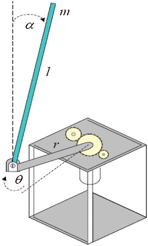
Figure 1: Setup schematic of rotary inverted pendulum
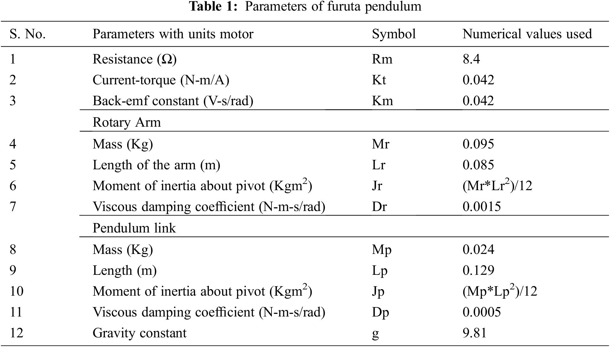
Fig. 2 represents the angular measurements of rotor arm angle, (θ in radians) with respect to base and pendulum angle, (α in radians). Tab. 1 enlists the parameters used for the analysis. The equations of motion for the FP (Eqs. (1)–(7)) is developed using Euler-Lagrange method and given below.
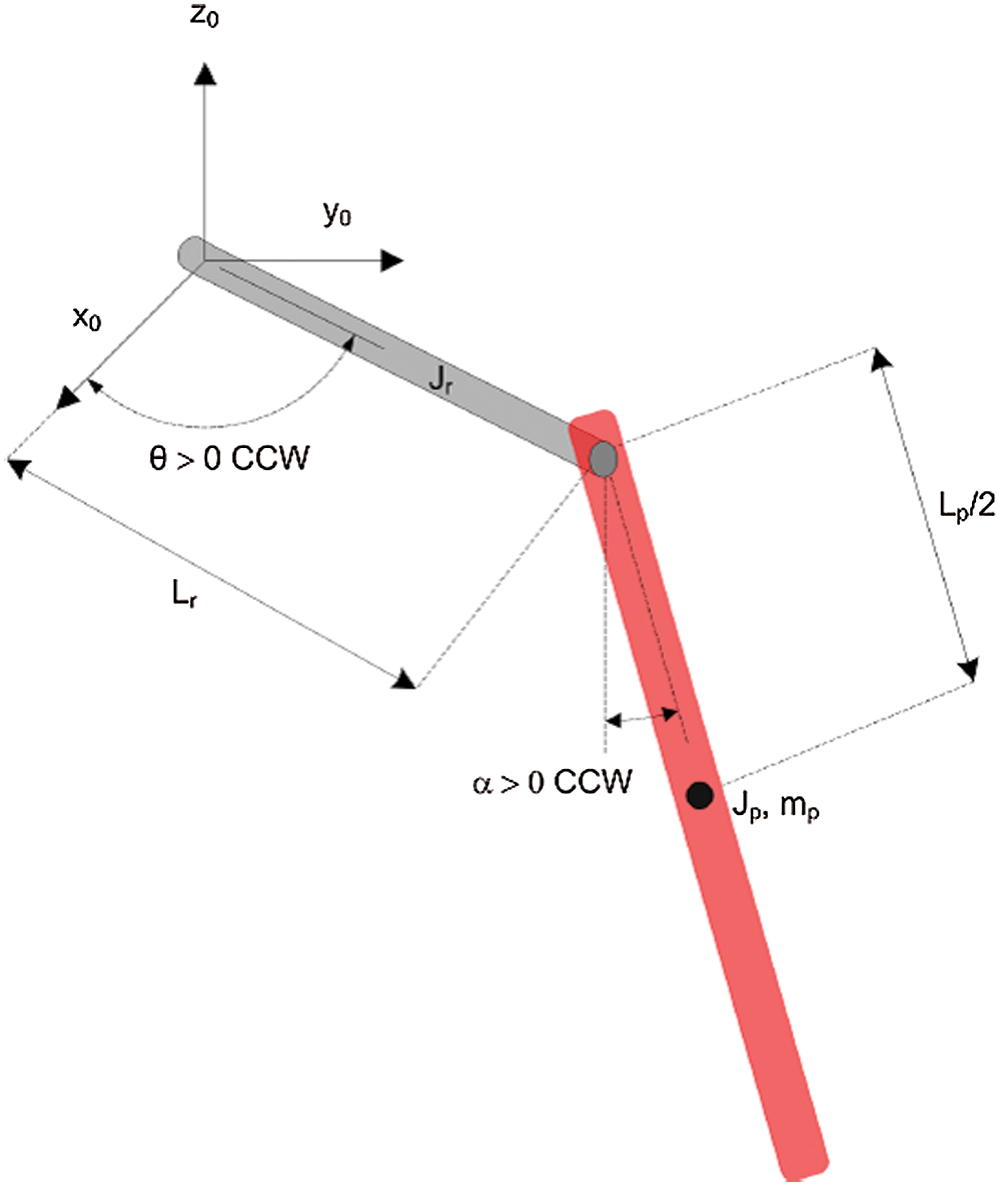
Figure 2: Schematic showing two degrees of freedom of rotary inverted pendulum
The nonlinear equations of motion are linearized about the operating point and are defined as
Solving the acceleration terms of rotor arm angle, θ and pendulum angle, α,
The state space equations describing the fourth-order continuous-time plant are
where, A is the system matrix, B and C are the output. State-variable models are made up of first-order differential equations that are interconnected.
And the corresponding states and output are defined to be
where θ represents the angular measurements of rotor arm angle, (in radians) with respect to base and α represents pendulum angle, (in radians);
The state space model of FP is obtained using the parameter values and system matrix of the model is
and the Eigen values are found to be
The plant mode is implemented in SIMULINK platform, which involves uncertainty parameters introduced to analyze the differences between stability factors of a nominal and perturbed plant by addition of feedback control changes the dynamic response of a linear process. Each uncertain parameter has a nominal value and an allowable level of tolerance expressed in terms of percentage and is enlisted Tab. 1.
The objective of the controller is framed as two tasks. viz.,
a) For Reference Tracking (RT), in which the controller attempts to adjust the input to negate the difference between the system model and the true plant.
b) For DR, in which the controller attempts to sustain the system at the point of action. i.e., upright position of pendulum arm in this case.
3.1 Linear Quadratic Gaussian Controller
A discrete LQG controller is designed where
a) The system is characterized to be a difference state and output equations.
b) Both the plant model and sensors, which are implanted to measure output variables, are subjected to stationary, independent, zero-mean Gaussian noises with covariance.
c) The cost function is defined with a quadratic function on state variables and input.
A quadratic function is of the form f(x) = ax2 + bx + c, where a, b, and c are real numbers with a ≠ 0. Further, if the variable factor is reduced the cost function will be quadratic.
The design of LQG comprises two components viz., LQR and Linear Quadratic Estimator (LQE). The LQR is designed to depreciate the quadratic performance index and finds the gain vector K of state space feedback law
which is applied to the time-invariant system described by the difference state and output equations
where v(k) is the noise component related to the plant and w(k) is the noise component related to the measurement respectively and are assumed to be stationary, independent zero-mean Gaussian white noise with covariance.
The discrete-time augmented model of the FP of fifth order is used in the LQR design and takes the state vector with the following form.
where q(k) is the discrete-time approximation of the position error integral
where q(kF) has the dimension of output y(k); TS is the sampling interval and e(k) represents the error signal between reference r(k) and output y(k). The augmented system is represented as
where the state vector
The optimal state feedback matrix
The augmented system is computed to be
The LQR design computed the K matrix to be
Consider the system represented by Eq. (13) and noise dynamics to be
whose input is considered to be a white noise η(k). Combining this Eq. (17) with Eq. (12)
The system with Kalman filter of sixth-order can be formed from the above Eq. (18) and is represented as
The Kalman filter of LQR as depicted in Fig. 3 which is designed by considering the quantization noises
for rotor arm angle and pendulum angle respectively. Also first order shaping filters are used as noise generators for rotor arm angle and pendulum angle and are assumed to be
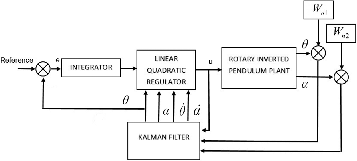
Figure 3: Block diagram of Kalman filter implementation for LQR controller
The system matrices are obtained as
The optimal gain matrix of Kalman filter is obtained by choosing suitable measurement noise and is of sixth order
3.3 LQ + H-Infinity (H∞) Filter
Consider the discrete-time system as represented by the Eq. (13), the H∞ filter considers the v(k) and w(k)as deterministic disturbances. The objective is to estimate
where Q and rare user-chosen symmetric positive definite co-variance matrices respectively and γ is user-defined positive scalar bound. The H∞ filter is expresses as [24]
and P is the discrete-time matrix algebraic Riccati equation solution and is given by
The H∞ filter will find a solution from matrix P for each step and must hold the following condition
The user-defined positive scalar bound, γ is chosen iteratively such that the Eigen values of the A(I − LC)matrix are inside the unit circle thus making the H∞ filter stable.
The control for the nonlinear system of the inverted FP has been implemented using Kalman and H∞ filter and LQR controller for inverted FP is designed using MATLAB/Simulink which is shown in Fig. 4. This section discusses the time response analysis, frequency response analysis, worst performance analysis, and robust stability analysis of the FP.
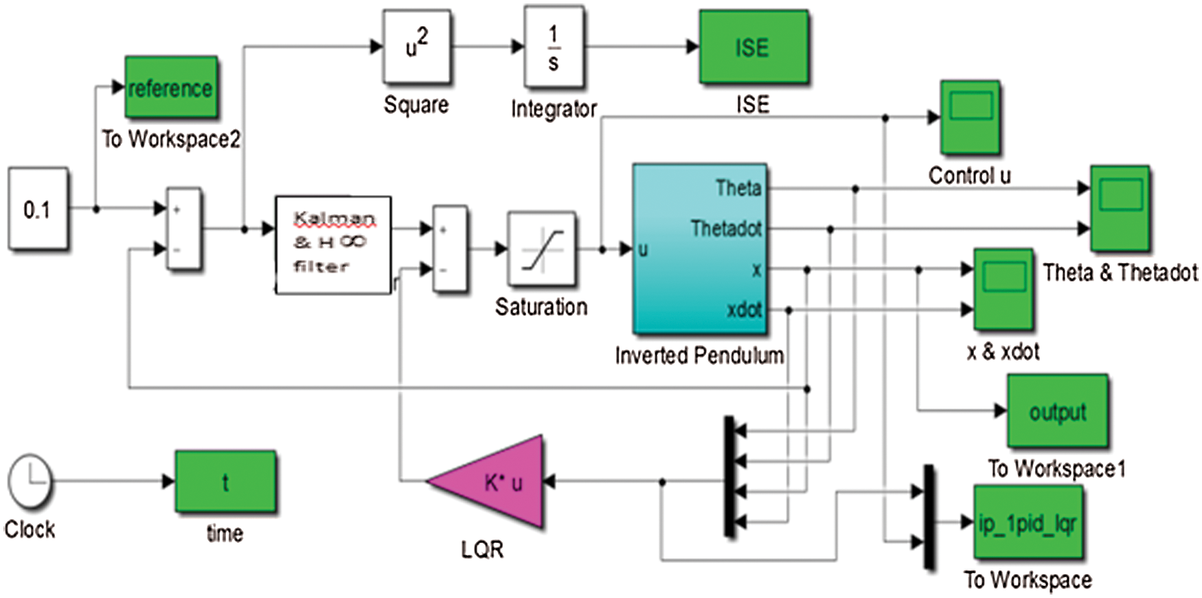
Figure 4: Simulink model of the proposed method
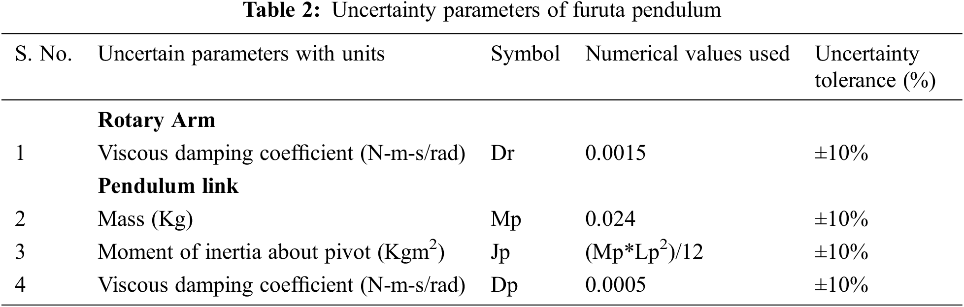
The RIP or FP is tested for instability due to model errors that arise because of the difference between the dynamics of nominal and perturbed system that occur due to the presence of uncertain dynamics. Hence four uncertain parameters are introduced to RIP and its nominal value and its uncertainty tolerances are enlisted in Tab. 2.
In Kalman filtering, the encoder generated white noises were approximated by first-order filters and its frequency response is shown in Fig. 5. It also depicts the fact that at the filters magnitude of these filters increases as frequency increases thereby it enables to include the effects of other possible noises that are inherent in the plant. The step response of the RIP which has two degrees of freedom i.e., the rotor arm angle, θ and Pendulum angle, α measured in degrees, is analyzed by implanting the LQG controller with Kalman filter in the closed loop structure. The smooth attempt of the controller action is shown in Fig. 6a as the input is generated as step input at 0 s And also a disturbance input introduced intentionally at 25 s. The corresponding step responses of rotor arm angle, θ and pendulum angle, α measured in degrees are displayed in Figs. 6b and 6c.
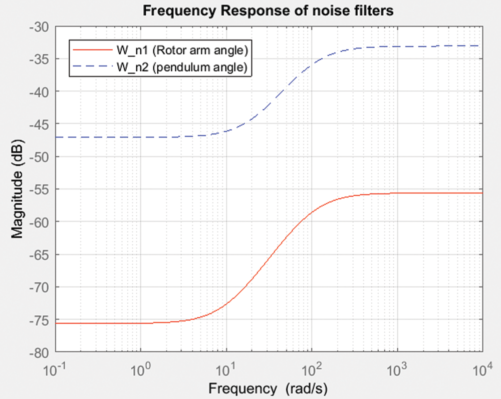
Figure 5: Frequency response of noise filters
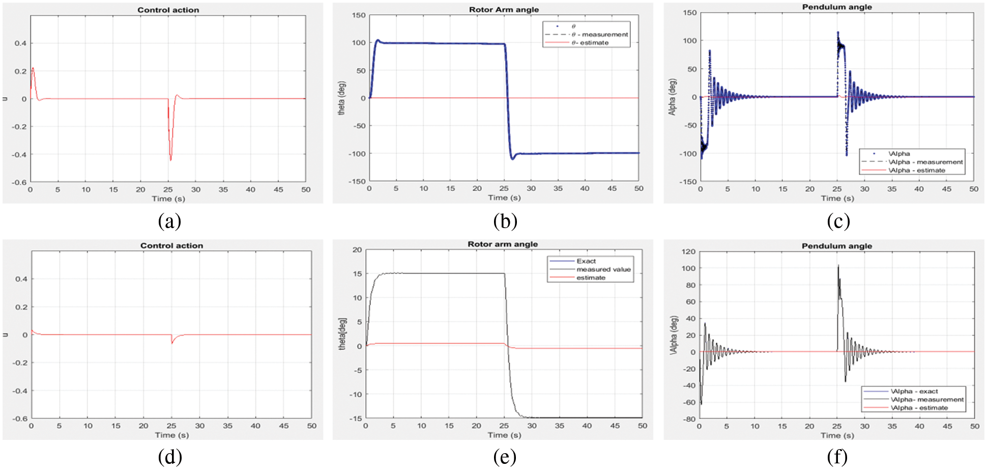
Figure 6: Controller action and step response of rotor arm angle, θ and pendulum angle, α. (a–c) shows the result of LQ + Kalman filter; (d–f) shows the result of LQ + H∞ filter
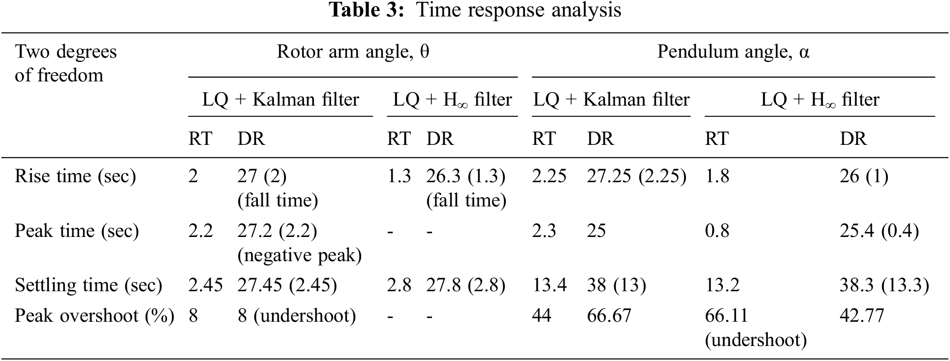
The step response is the time of a system’s outputs when its inputs go from 0 to 1 in a very short period of time. The concept may be extended through an evolution parameter to the abstract mathematical notion of a dynamic system. The step response analysis also shows that the rotor arm angle, θ is having a peak time at 2.2 s represents the time necessary to achieve the first peak, i.e., the first oscillating cycle peak and the settling time is recorded to be 2.45 s which, is the time spent on an ideal instantaneous step input by the time the amplifier output was inserted and kept in a certain error band. It exhibits the negative undershoot for disturbance and a quick fall time at 25 s which represents, that the time needed to decline the amplitude of a pulse from a given value to a defined value. The maximum peak overshoot is 8% and pendulum angle, α is having a peak time of 2.3 s and settles slower comparatively at 13.4 s and the maximum peak overshoot for reference input and disturbance input is found to be 44% and 66.67% respectively. The step response of rotor arm angle, θ is exhibiting an equal rise in amplitude for both reference and disturbance inputs carrying their respective directions whereas the pendulum angle, α is showing up an initial rise in opposite direction in response to both reference input is a signal provided to the control system that represents the intended controlled output value and disturbance input due to the influence of zero in the right half-plane i.e., non-minimum phase of the system.
The step response of the RIP is also analyzed by implanting the LQG controller with H∞ filter. The smooth attempt and reduced amplitude effort of the controller action is shown in Fig. 6d for step and disturbance introduced in similar fashion as before. The corresponding step responses of rotor arm angle, θ and pendulum angle, α measured in degrees are displayed in Figs. 6e and 6f. Tab. 3 enlists the time domain specifications with respect to two degrees of freedom viz., rotor arm angle, θ and pendulum angle, α for both filter configurations.
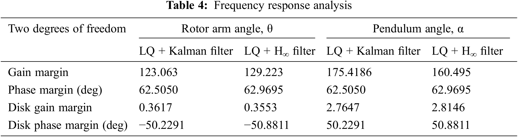
The frequency response analysis of the closed loop system is shown in Fig. 7 which reveals that the system is having a gain margin of 123.06 deg and phase margin of 62.5 deg for LQ + Kalman filter and a gain margin of 129.223 deg and phase margin of 62.96 deg for LQ+ H∞ filter. Also the stability margins are tabulated in Tab. 4 for both filter configurations. The magnitude plot of sensitivity with respect to pendulum angle, α is shown in Fig. 8 depicts that the sensitivity is of small magnitude at low frequencies and ensures that error and disturbance effect can be tracked and used for noise suppression and to reduce the effect of measurement noise introduced to the system. The magnitude plot of Integral of error is shown in Fig. 9 shows that the constant magnitude at low frequencies ensures that controller design is used to influence the location of unstable poles or zeroes to the left half of s-plane. Fig. 10 shows the sensitivity of control action due to reference input which, is between −100 to −35, rotor arm angle, θ and pendulum angle, α.
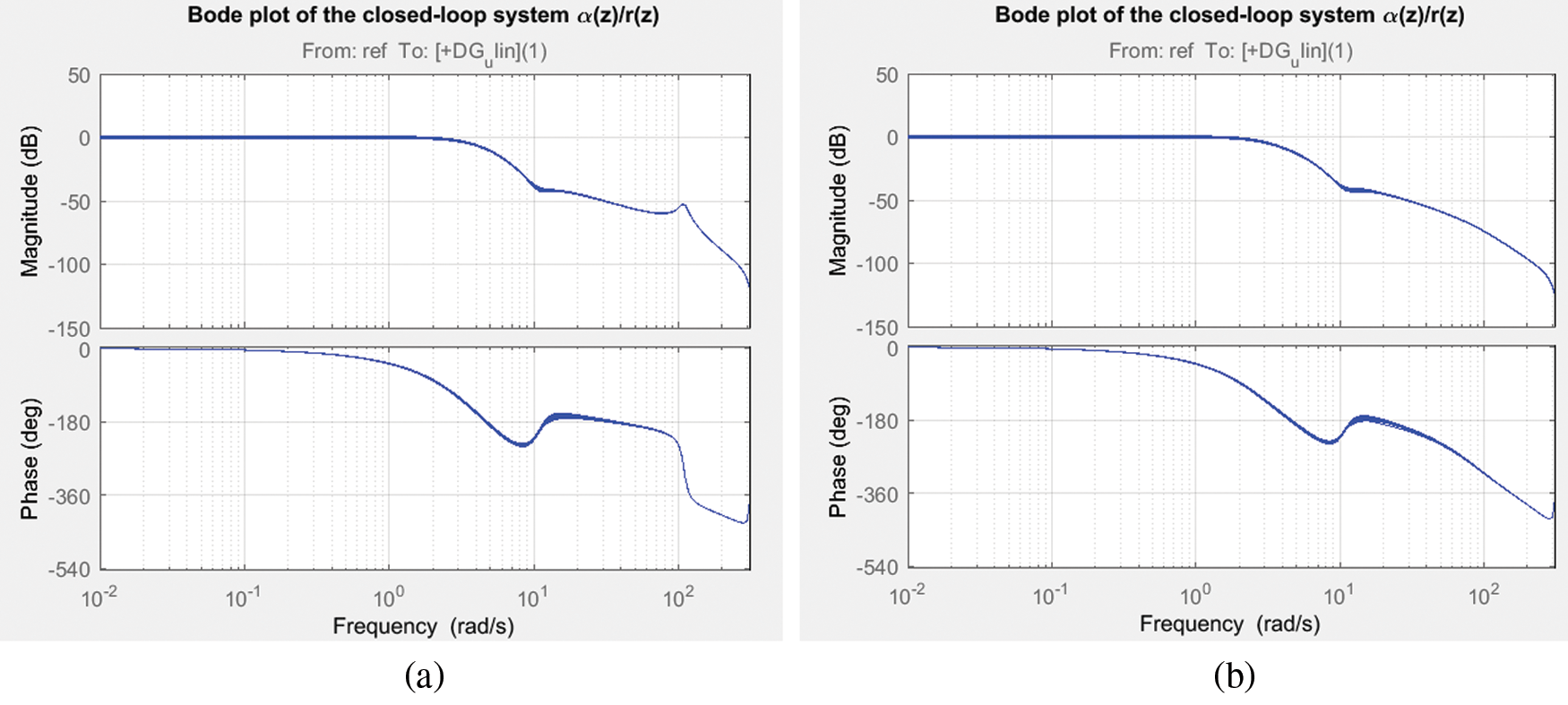
Figure 7: Bode plot of closed-loop system (a) LQ + Kalman filter; (b) LQ + H∞ filter
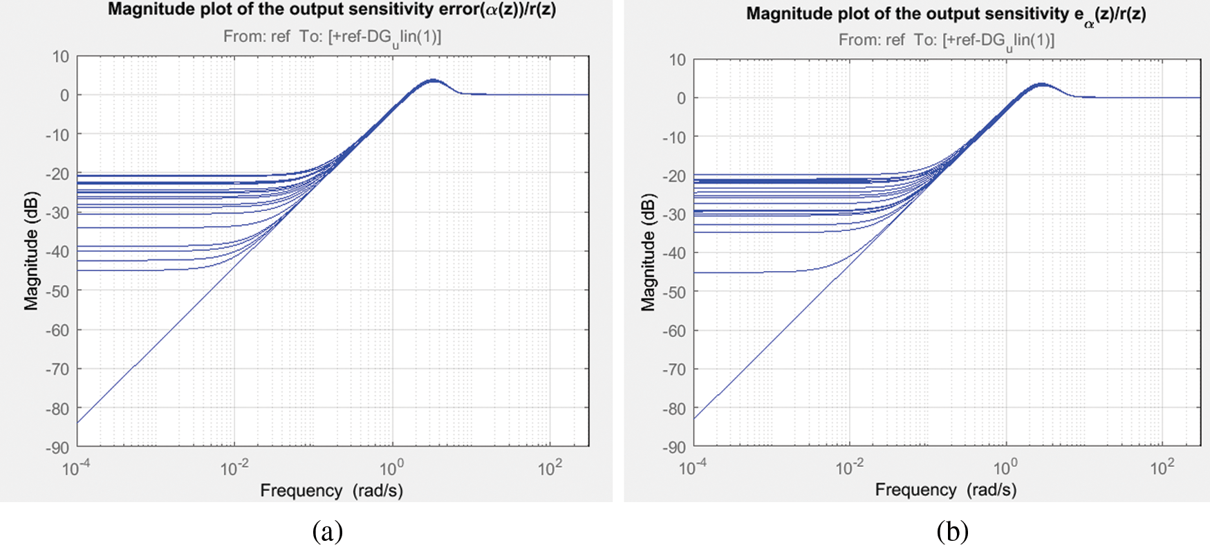
Figure 8: Magnitude response of output sensitivity error (a) LQ + Kalman filter; (b) LQ + H∞ filter
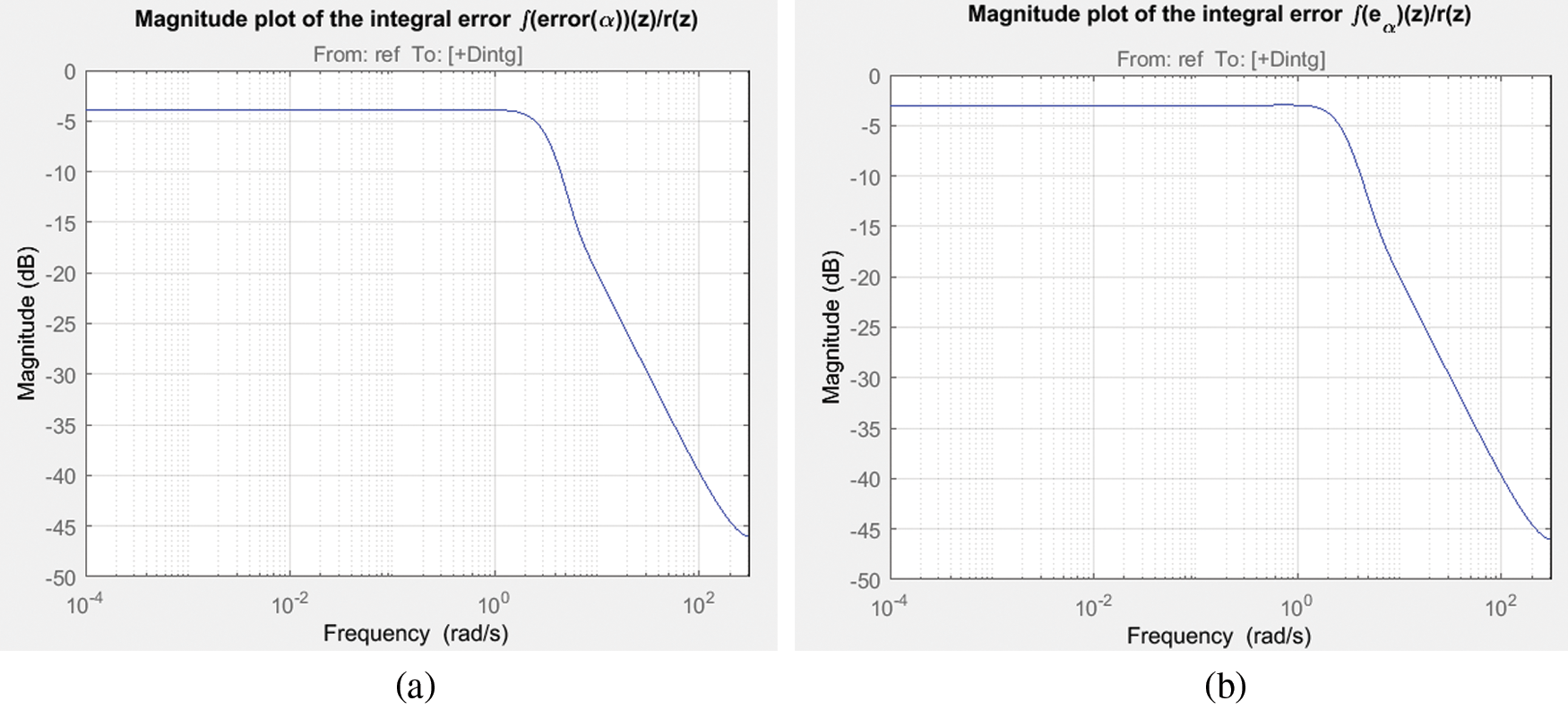
Figure 9: Magnitude response of integral error (a) LQ + Kalman filter; (b) LQ + H∞ filter
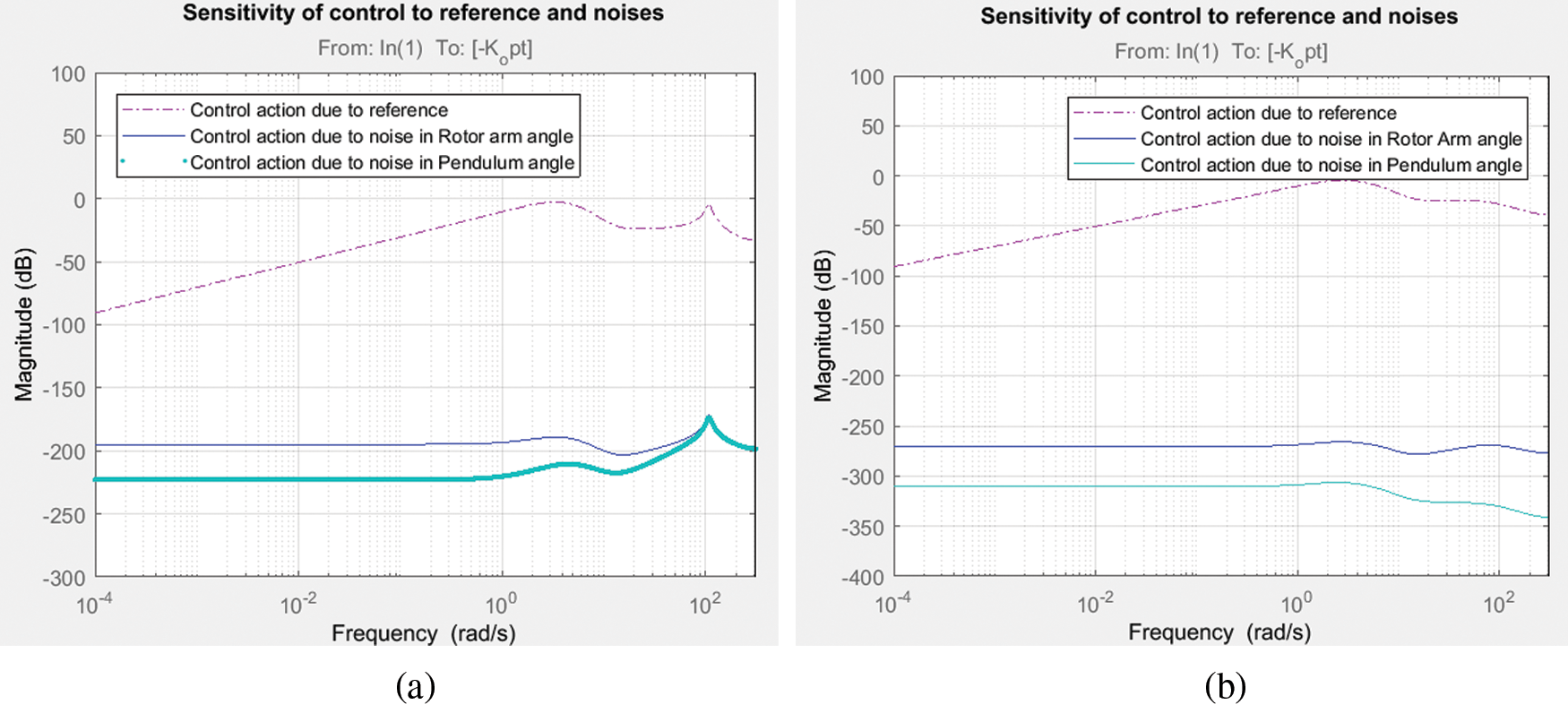
Figure 10: Magnitude response of control sensitivity due to input and noises in output (a) LQ + Kalman filter; (b) LQ + H∞ filter
4.3 Analysis of Robust Stability
The robust stability analysis is reported to have a peak value of structured singular value, which is found to be 0.2024 and 0.2016 for LQ + Kalman filter and LQ + H∞ filter respectively and is best viewed from Fig. 11. This indicates the model can tolerate up to 494% of model uncertainty with LQ + Kalman filter and 496% of uncertainty for LQ + H∞ filter. Also the peak value of structured singular value is less than one which indicates that the system is robustly stable. We employ the idea of performance margin that demonstrates a degree of uncertainty that has defined performance in a robust stability. As per this analysis of the filters in LQR, the degrees of freedom should be evaluated, which shows that slightly LQ + H∞ filter is tolerate by the values of the modeled uncertainty.
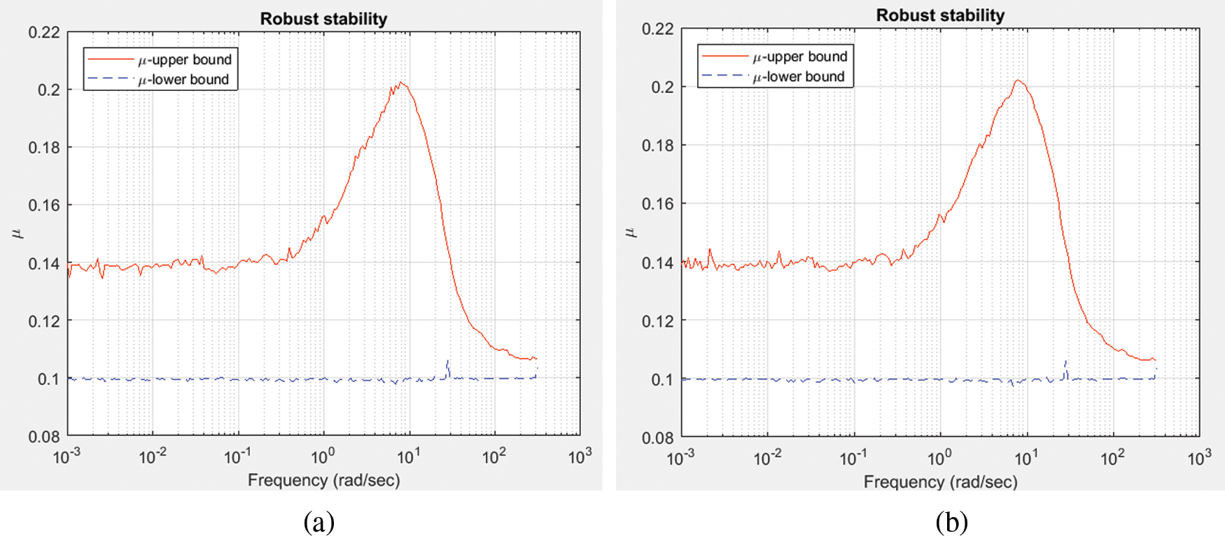
Figure 11: Robust stability analysis of closed loop system (a) LQ + Kalman filter; (b) LQ + H∞ filter
From Figs. 10 and 11, the proposed controller provides peak value of structured singular value is less than one which indicates that the system is robustly stable. So, this controller is the best solution for worst and robust stability case.
4.4 Worst Performance Analysis
The FP or RIP is tested for its worst performance in frequency domain by the largest possible gain called ‘worst gain’. The worst case analysis is carried out by determining all the component values at their end-tolerance limits, which show the worst-case outcome. Collection features may be used to detect variance from nominal worst case output, like the minimum, maximum or threshold variations, to minimize the number of simulation runs. This gain deals with uncertainty that influence due to unmodeled dynamics of the non-linear, non-minimum phase RIP for both degrees of freedom. Also, it enables to assess the robust performance by considering the worst case margin of the system. The robust stability analysis for both configurations with its upper and lower bound is recorded in Fig. 12 and is found to be less than 1 and proves the system is robust stable. Whilst the Kalman filter is the best suitable linear estimator for the least mean-square-error sense, independent of gaussianity, when process and measurement covariance. Also, H∞ filter minimizes the estimation error. Fig. 13 shows the magnitude response of sensitivity of control action with respect to the reference and noise in the outputs of RIP and recorded to be of in smaller magnitudes at low frequencies with significant differences for both filter configurations. The time response of rotor arm angle and Pendulum angle, α for step input with worst case gain and random 10 values are displayed in Figs. 14 and 15 respectively for both filter configurations.
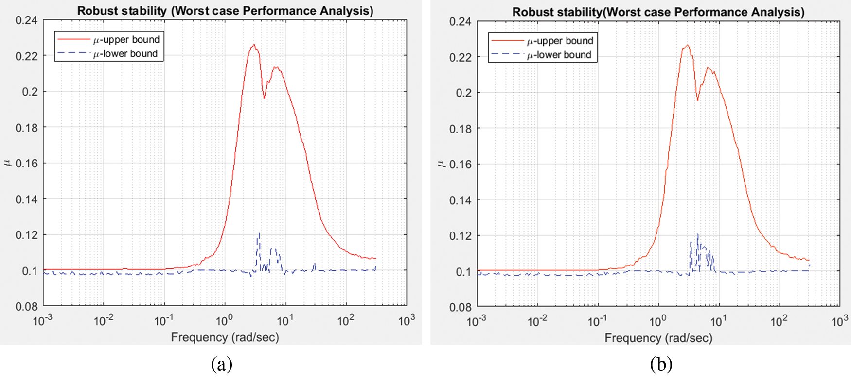
Figure 12: Robust stability analysis of uncertain closed-loop system (a) LQ + Kalman filter; (b) LQ + H∞ filter
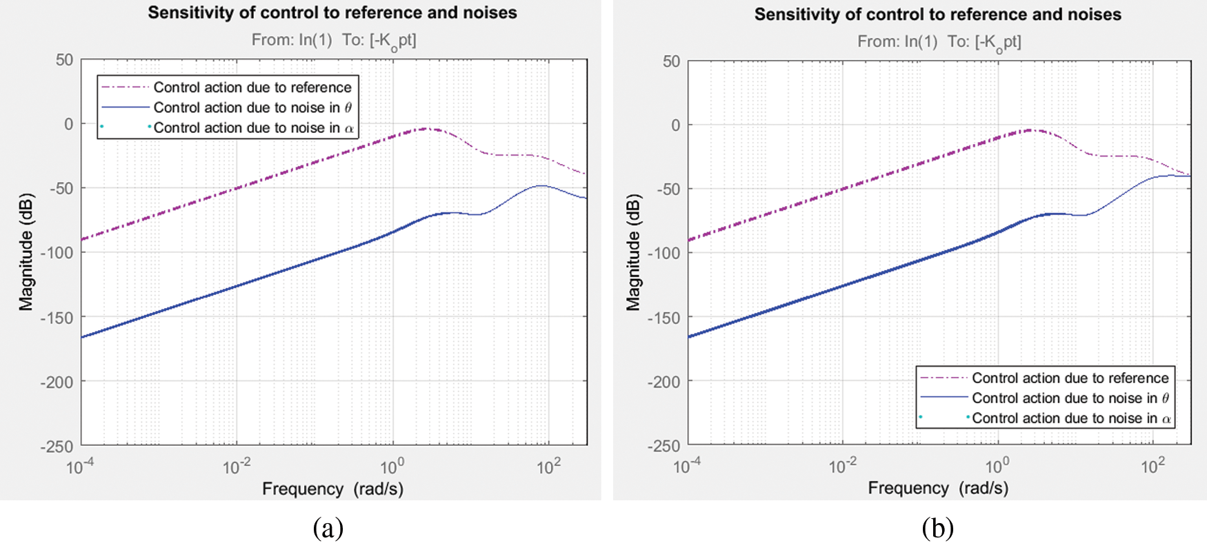
Figure 13: Magnitude response of sensitivity of control action due to input and noises in output (a) LQ + Kalman filter; (b) LQ + H∞ filter
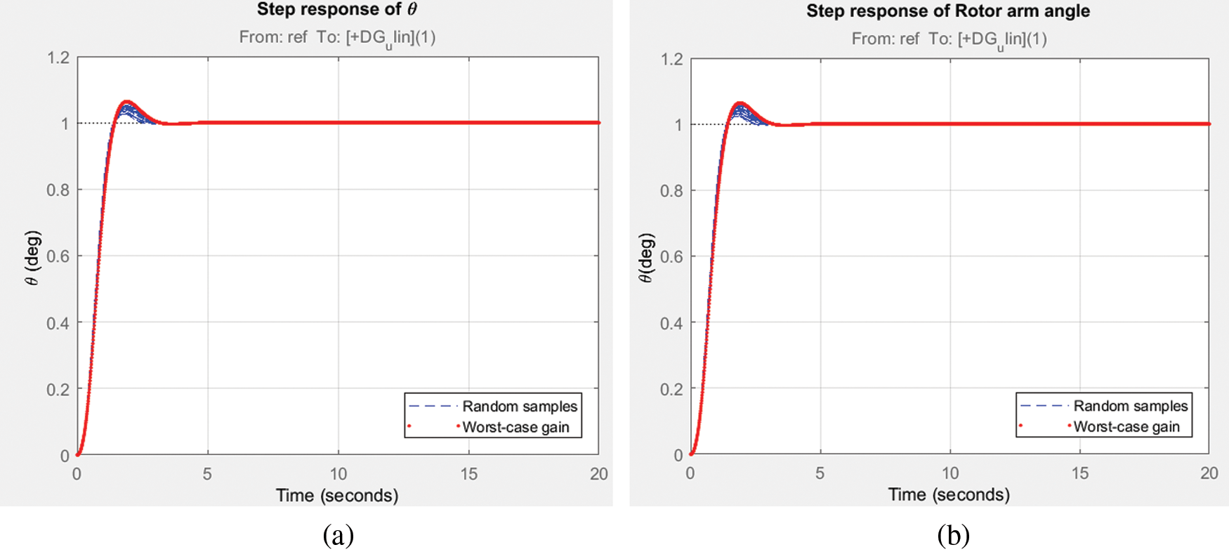
Figure 14: Step response of rotor arm angle, θ; (a) LQ + Kalman filter; (b) LQ + H∞ filter

Figure 15: Step response of Pendulum angle, α. (a) LQ + Kalman filter; (b) LQ + H∞ filter
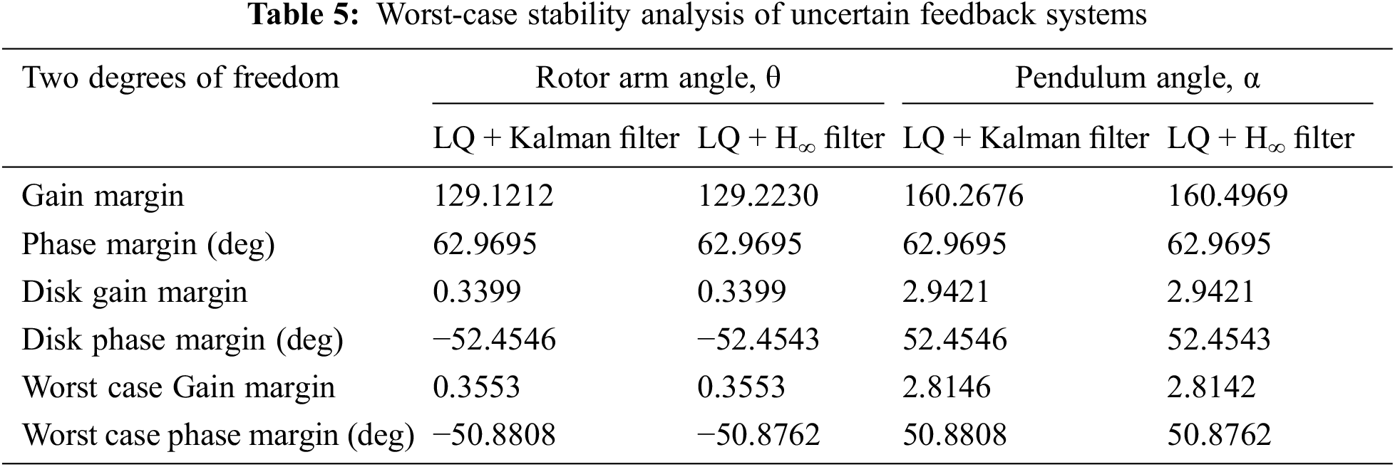
Tab. 3 enlists the time domain specifications with respect to two degrees of freedom viz., Rotor arm angle, θ and Pendulum angle, α for both filter configurations of rise time 1.3 s in RT of LQ + H∞ filter, peak time is 0.8 in LQ + H∞ filter in α, settling time is low in LQ + Kalman filter which is 2.45 s and peak overshoot is represents satisfactory in α. Tab. 4 enumerates the Frequency specifications and margins represents that according to the θ, LQ + H∞ filter has slightly greater than the LQ + Kalman filter as well as in α except gain margin. And Tab. 5 lists the worst case stability specifications for both filter configurations represents that the LQ + H∞ filter has slightly high worst-case stability analysis of uncertain feedback systems. The LQR with Kalman filter and H∞ filter had been attempted for RIP, which is an under-actuated non-minimum phase non-linear process. The results reveal that as the probability density function of the noise is a known parameter for the user that gives the user to obtain a statistically optimal state estimate. The kalman filter does not give clues on limiting the worst-case estimation error 0.335 in θ and 2.8146 in α for gain margin. The H∞ filter depends strongly on the states which are to be estimated. Also the H∞ filter outperforms the kalman filter in terms of DR and noise suppression specifications and robustness. The kalman matrix does not increase the Q part of the filter when tolerance is added to un-modelled noise and dynamics whereas the H∞ filter behaves as Kalman filter by choosing γ → ∞ and hence it behaves as robust version of kalman filter.
Funding Statement: The authors received no specific funding for this study.
Conflicts of Interest: The authors declare that they have no conflicts of interest to report regarding the present study.
1. E. J. Davison, “Benchmark problems for control system design,” International Federation of Automatic Control Report, pp. 37–41, 1990. [Google Scholar]
2. C. C. Hung and B. Fernandez, “Comparative analysis of control design techniques for acart-inverted-pendulum in real-time implementation,” American Control Conf., San Francisco, CA, USA, pp. 1870–1874, 1993. [Google Scholar]
3. D. E. Kirk, “Iterative numerical techniques for finding optimal controls and trajectories,” in Optimal Control Theory: An Introduction, 13th ed, Mineola, NY, USA: Dover Publications Inc., pp. 329–416, 2012. [Google Scholar]
4. D. Angeli, “Almost global stabilization of the inverted pendulum via continuous state feedback,” Automatica, vol. 37, no. 7, pp. 1103–1108, 2001. [Google Scholar]
5. B. Srinivasan, P. Huguenin and D. Bonvin, “Global stabilization of an inverted pendulum–control strategy and experimental verification,” Automatica, vol. 45, no. 1, pp. 265–269, 2009. [Google Scholar]
6. K. J. Astrom and K. Furuta, “Swinging up a pendulum by energy control,” Automatica, vol. 36, no. 2, pp. 287–295, 2000. [Google Scholar]
7. B. S. Cazzolato and Z. Prime, “On the dynamics of the furuta pendulum,” Journal of Control Science and Engineering, vol. 2011, pp. 1–8, 2011. [Google Scholar]
8. S. K. Das and K. K. Paul, “Robust compensation of a cart–inverted pendulum system using a periodic controller: Experimental results,” Automatica, vol. 47, no. 11, pp. 2543–2547, 2011. [Google Scholar]
9. G. Li and X. Liu, “Dynamic characteristic prediction of inverted pendulum under thereduced-gravity space environments,” Acta Astronautica, vol. 67, no. 6, pp. 596–604, 2010. [Google Scholar]
10. M. Park, Y. J. Kim and J. J. Lee, “Swing-up and LQR stabilization of a rotary inverted pendulum,” in 16th Int. Symp. on Artificial Life and Robotics, Beppu, Japan, vol. 16, no. 1, pp. 94–97, 2011. [Google Scholar]
11. Y. F. Chen and A. C. Huang, “Adaptive control of rotary inverted pendulum system with time-varying uncertainties,” Journal of Nonlinear Dynamics, vol. 76, no. 1, pp. 95–102, 2013. [Google Scholar]
12. M. Bettayeb, C. Boussalem, R. Mansouri and U. M. Al-Saggaf, “Stabilization of an inverted pendulum-cart system by fractional PI-state feedback,” ISA Transactions, vol. 53, no. 2, pp. 508–516, 2014. [Google Scholar]
13. L. B. Prasad, B. Tyagi and H. O. Gupta, “Optimal control of nonlinear inverted pendulum system using PID controller and LQR: Performance analysis without and with disturbance input,” International Journal of Automation and Computing, vol. 11, no. 6, pp. 661–670, 2014. [Google Scholar]
14. L. Chrif and Z. M. Kadda, “Aircraft control system using LQG and LQR controller with optimal estimation-Kalman filter design,” Procedia Engineering, vol. 80, pp. 245–257, 2014. [Google Scholar]
15. C. Aguilar-Avelar and J. Moreno-Valenzuela, “New feedback linearization-based control for arm trajectory tracking of the furuta pendulum,” IEEE/ASME Transactions on Mechatronics, vol. 21, no. 2, pp. 638–648, 2015. [Google Scholar]
16. P. Ordaz and A. Poznyak, “Adaptive-robust stabilization of the furuta’s pendulum via attractive ellipsoid method,” Journal of Dynamic Systems, Measurement and Control, vol. 138, no. 2, pp. 1–8, 2016. [Google Scholar]
17. P. D. Mandić, M. P. Lazarević and T. B. Šekara, “D-decomposition technique for stabilization of furuta pendulum: Fractional approach,” Bulletin of the Polish Academy of Sciences: Technical Sciences, vol. 64, no. 1, pp. 189–196, 2016. [Google Scholar]
18. V. M. Hernández-Guzmán, M. Antonio-Cruz and R. Silva-Ortigoza, “Linear state feedback regulation of a furuta pendulum: Design based on differential flatness and root locus,” IEEE Access, vol. 4, pp. 8721–8736, 2016. [Google Scholar]
19. I. Paredes, M. Sarzosa, M. Herrera, P. Leica and O. Camacho, “Optimal-robust controller for furuta pendulum based on linear model,” in IEEE Second Ecuador Technical Chapters Meeting, Salinas, Ecuador, pp. 1–6, 2017. [Google Scholar]
20. M. F. Hamza, H. J. Yap and I. A. Choudhury, “Cuckoo search algorithm based design of interval type-2 fuzzy PID controller for furuta pendulum system,” Engineering Applications of Artificial Intelligence, vol. 62, pp. 134–151, 2017. [Google Scholar]
21. J. Ismail and S. Liu, “Efficient planning of optimal trajectory for a furuta double pendulum using discrete mechanics and optimal control,” IFAC-PapersOnLine, vol. 50, no. 1, pp. 10456–10461, 2017. [Google Scholar]
22. C. Hajiyev, H. E. Soken and S. Y. Vural, “Linear quadratic regulator controller design,” in State Estimation and Control for Low-Cost Unmanned Aerial Vehicles, 1st ed, Switzerland: Springer, pp. 171–200, 2015. [Google Scholar]
23. A. K. Patra, S. S. Biswal and P. K. Rout, “Backstepping linear quadratic Gaussian controller design for balancing an inverted pendulum,” IETE Journal of Research, vol. 65, no. 3, pp. 1–15, 2019. [Google Scholar]
24. D. Simon, “The H∞ filter,” in Optimal State Estimation: Kalman, H∞, and Nonlinear Approaches, 6th ed, Hoboken, NJ, USA: John Wiley & Sons, Inc., pp. 333–394, 2006. [Google Scholar]
 | This work is licensed under a Creative Commons Attribution 4.0 International License, which permits unrestricted use, distribution, and reproduction in any medium, provided the original work is properly cited. |