DOI:10.32604/csse.2022.023617
| Computer Systems Science & Engineering DOI:10.32604/csse.2022.023617 | |
| Article |
Optimized Gated Recurrent Unit for Mid-Term Electricity Price Forecasting
1Department of Electrical Engineering, Faculty of Engineering, Universiti Malaya, 50603, Malaysia
2Department of Electrical Engineering, Main Campus, Iqra University, Karachi, 75300, Pakistan
*Corresponding Author: Anis Salwa Mohd Khairuddin. Email: anissalwa@um.edu.my
Received: 14 September 2021; Accepted: 01 December 2021
Abstract: Electricity price forecasting (EPF) is important for energy system operations and management which include strategic bidding, generation scheduling, optimum storage reserves scheduling and systems analysis. Moreover, accurate EPF is crucial for the purpose of bidding strategies and minimizing the risk for market participants in the competitive electricity market. Nevertheless, accurate time-series prediction of electricity price is very challenging due to complex nonlinearity in the trend of electricity price. This work proposes a mid-term forecasting model based on the demand and price data, renewable and non-renewable energy supplies, the seasonality and peak and off-peak hours of working and non-working days. An optimized Gated Recurrent Unit (GRU) which incorporates Bagged Regression Tree (BTE) is developed in the Recurrent Neural Network (RNN) architecture for the mid-term EPF. Tanh layer is employed to optimize the hyperparameters of the heterogeneous GRU with the aim to improve the model’s performance, error reduction and predict the spikes. In this work, the proposed framework is assessed using electricity market data of five major economical states in Australia by using electricity market data from August 2020 to May 2021. The results showed significant improvement when adopting the proposed prediction framework compared to previous works in forecasting the electricity price.
Keywords: Deep learning; energy management; machine learning; prediction
The forecast of electricity price projection is an important element of expectations for policy makers, governments, and financial market participants. Electricity price forecasting (EPF) has become an important information to manage the deregulated electricity market, complex renewable energy and emission policy objectives. This is because, accurate and consistent price forecasting will minimize risk, maximize profit for the day-to-day market, improve bidding and production measures [1]. In several countries, deregulations of the electricity sector have been developed to enhance congestion control, facilitate renewable energy, and maximize the resource allocation of the power system. In addition, EPF provides vital information to all stakeholders in the power sector marketplace since the accuracy of EPF influenced the performance and rational analysis of energy resource optimization. Besides, accurate EPF can improve wholesale electricity price bidding strategy and production which can increase the profits in day-ahead trading and energy management. Usually, power portfolio managers are interested with short-term and mid-term price forecasts. The short-term forecasts (intra-day) are the key elements in day-to-day market operations, especially for bidding at a power exchange or for executing effective demand response. Meanwhile, the mid-term forecasting which can range from several weeks to several months ahead are used for planning purposes such as the tuning of mid-term plans and resources allocation, risk management and the valuation of exchange traded futures and bilateral contracts. This is due to high saturation of intermittent technologies and the evolving concerns related to resource adequacy in the longer-term. These forecasting operations will affect the baseload electricity price, such as the peakload price, the average price for the 24 h of the day or the baseload price [2].
In general, time series forecasting is analyzing time series data via modelling and statistics approach to aid strategic decision-making process. Time series forecasting incorporates information related to historical values and associated patterns to foresee future activity [3,4]. Nowadays, researchers are capable of employing and extracting complex information from time series data to solve various problems such as wind speed prediction [4], stock market prediction [3,5–7], and forecasting electricity prices [8,9]. Time series models have been widely used to forecast electricity prices, although they can be challenging due to large variations [10–19]. Existing statistical techniques tried to reveal the specific pattern of historic power price utilizing curve fitting. For instance, German electricity market has tested a k-factor Guégan Introduced Generalized Autoregressive Conditionally Heteroskedastic (GIGARCH) for forecasting electricity price [10,11]. An iterative neural network methodology is also adopted along with this combinatorial neural network-based prediction technique to forecast upcoming electricity price. The advantages of this method include good precision, model functionality, and reliability. Meanwhile, Auto-regressive Integrated Moving Average (ARIMA) was proposed for electricity and power load forecasting [13,14,16,18]. However, application of statistical models had shown to be challenging when predicting multi-dimensional nonlinear price of electricity since they are mainly based on linear equations. Moreover, statistical methods are inadequate for solving nonlinear multi-dimensional data for prediction purpose, as its more suitable in handling linear data [20].
In time series analysis, machine learning models have shown to perform better than statistical methods. Support Vector Machine (SVM) was adopted in [17,20,21] for load and electricity forecasting. The other common machine learning models applied in EPF are support vector regression (SVR) [22–24] and artificial neural network (ANN) [19,25,26]. Hybrid models of ANN are used to predict electricity load and price such as adaptive network-based fuzzy inference system (ANFIS) and Backtracking Search algorithm (BSA) [27]. However, the abovementioned conventional machine learning models are inadequate for complex and nonlinear problems. Recurrent neural network (RNN) which is a deep learning technique with a recurrent feedback network has shown to perform better when dealing with time series data compared to conventional machine learning algorithm [28]. The work in [18] proposed a Deep Belief Network (DBN) for electricity price forecasting. On the other hand, the work in [15], proposed LSTM network for electricity price forecasting. Nevertheless, the performance of the proposed models from previous methods can still be improved to achieve more accurate results when dealing with complex and nonlinear electricity market fluctuations.
Therefore, this paper proposes an optimized GRU consisting of RNN with Bagged Regression Tree forecasting model for electricity price prediction. The bagged trees regression is applied to predict nonlinear data which is further optimized by using GRU RNN network. Then the tanh layer is utilized to optimize the hyperparameters of the heterogeneous GRU to improve the model’s performance, error reduction and predict the spikes. Contributions of this study include:
• Improvement of the prediction performance by tuning the nonlinear degree of the feature effects of demand, seasons, fuel supply, renewable and non-renewable energy, peak and off-peak hours of forecasting,
• Integration of Bagged Trees and GRU in RNN to handle complex nonlinear features of electricity price.
• Prediction of the unusual price spikes by adopting GRU and Tanh function layers which optimize the hyper parameters of deep neural networks.
This paper is structured as follows. Section 2 explains the proposed methodology; Section 3 presents the results and discussions. Finally, Section 4 provides the conclusion of this work.
This work proposed a forecasting framework for mid-term EPF for five states in Australia which includes pre-processing module, Bagged Trees Ensemble (BTE) algorithm, Recurrent Neural Network (RNN) and Gated Recurrent Unit (GRU). The electricity market dataset is divided into three components: training set, validation set and test set. The workflow of the proposed framework is shown in Fig. 1.
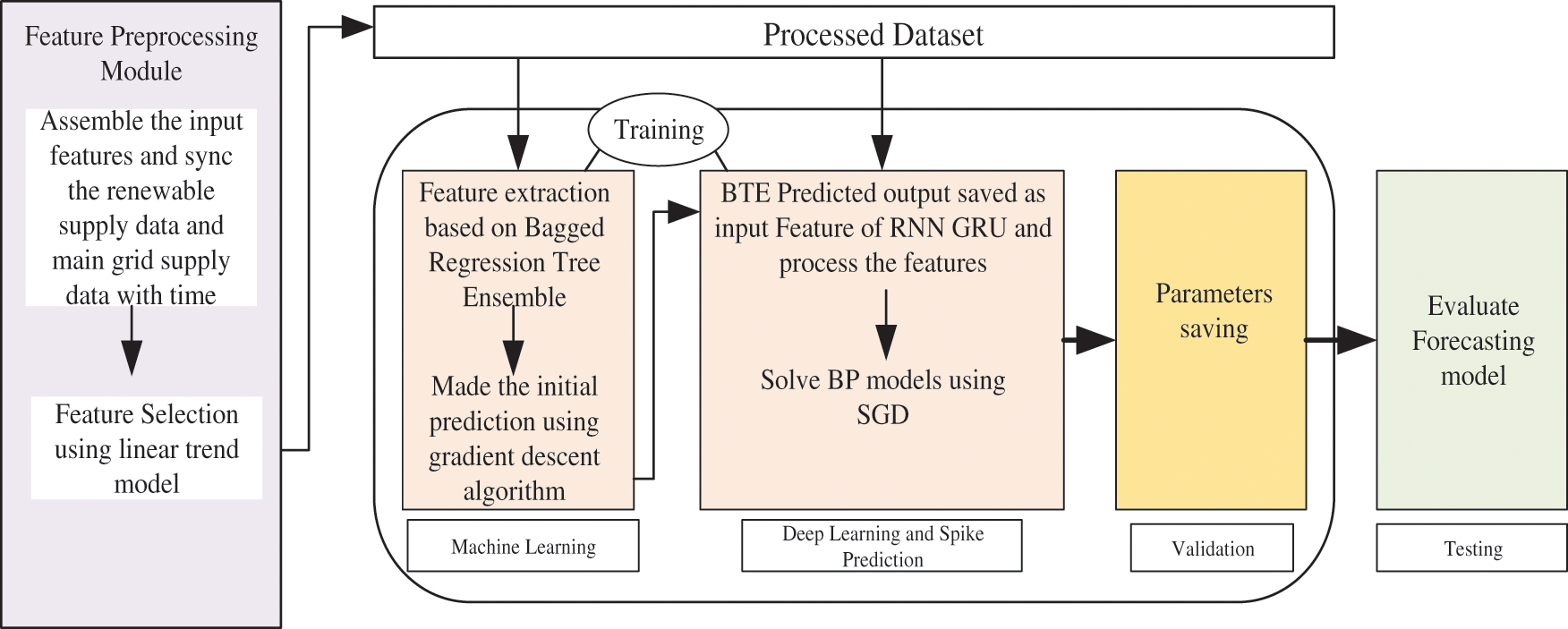
Figure 1: Flow diagram of the proposed framework
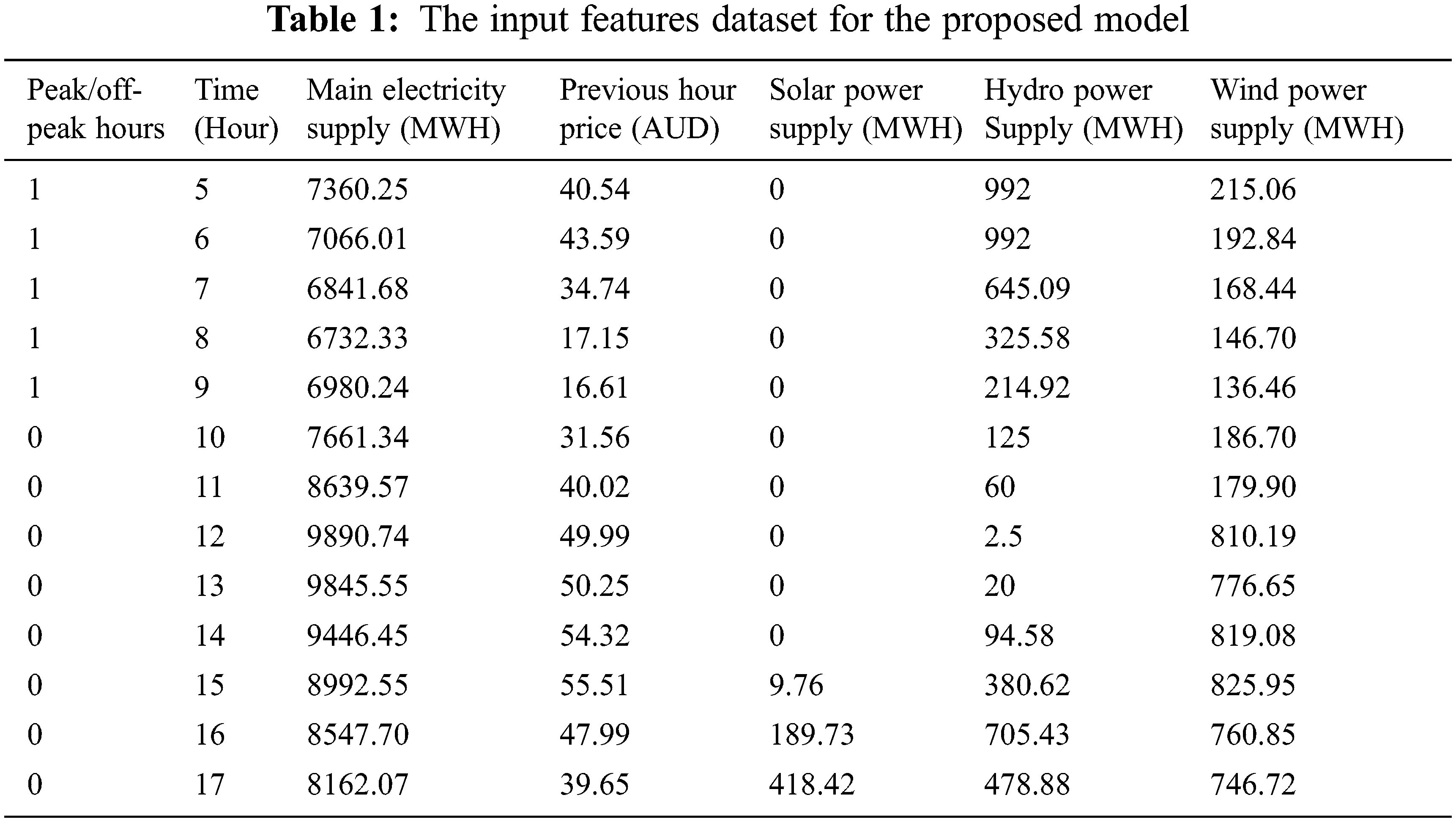
The proposed forecasting model is developed based on information of the demand and price data in megawatts (MW) and Australian dollar (AUD) from five states in Australia (NSW, QLD, SA, TAS, VIC). Furthermore, we considered renewable and non-renewable energy supplies data in megawatts (MW) which substantially impact pricing electricity. Besides that, the seasonality and peak and off-peak hours of working and non-working days were also considered. Data clusters are usually formed by the input features may present when accumulating unprocessed data due to high dimensions, outliers, and missing values, which contributes to instability in the forecasting performance [29]. Therefore, data clusters need to be pre-processed to aid the prediction process. Hence, in this work, a linear trend model is applied to identify effective pattern of features for the prediction process. Example of dataset adopted in this work is tabulated in Tab. 1.
The linear trend method acts with the trend precisely and show the trend without any assumption. The input dataset used in this work are the residual seasonality, peak and off-peak hour and renewable energy trend in time series dataset. Let p1 = t1 and q1 = 0. The equations for the feature processing are described in Eqs. (1)–(7). Where pi is the approximation level of the series at time t, qi is the estimation of the trend (slope) of the series at time t, α is the smoothing parameter of the level 0 < α ≤ 1 and β is the smoothing parameter of the level 0 ≤ β ≤ 1. i denotes the seasonality and t is the hour of observation.
Let p1 = t1 and q1 = 0. An alternative form of these equations are;
where,
Note that if β = 0, then the linear modecan be considered as single exponential smoothing model.
2.2 Bagged Trees Ensemble (BTE)
Bagged Trees Ensemble (BTE) algorithm is adopted to generate several bootstrap samples and trains classifiers on the new learning sets. Then, BTE algorithm computes the mean predictions for a sequential output or performs a plurality for a class outcome. Assuming the training set is defined as A{(pm, qm), m

The classifiers are also defined as regression trees (decision trees). In this work, the proposed bagged tress implemented 5 folds cross-dation. Then, the number of RT (chosen N = 30) and the minimal leaf size (selected Gmin = 8) are applied. Each regression tree was built using a bootstrap sample selected uniformly fromhe input data. Further, the bagging method averaged the learners’ outputs to obtain a single forecast. This technique is called bagging and Tab. 2 presents the bagging algorithm applied in this work.
2.3 Gated Recurrent Unit (GRU)
As RNN is recurrent in nature, it wos much the same way for all inputs, while the output of the input data is dependent on the previous calculations. After generating the output data, it is replicated and revert back into the recurrent network unit. RNN count the present input and the output acquired from the last input while it makes logical decision. RNNs can utilize the internal state (memory) to evaluate input variables, which is different from feedforward neural network [31,32]. In recurrent neural network, all of the inputs are connected with one another, which distinguishes it from the other neural networks.
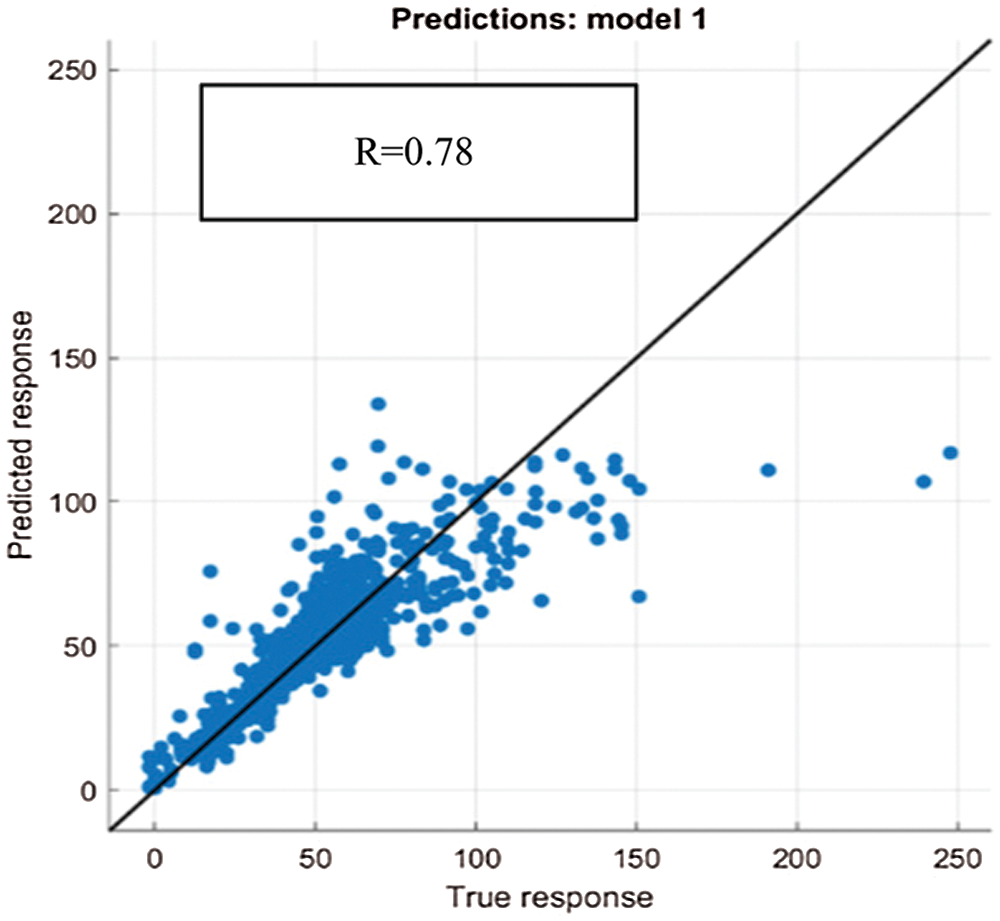
Figure 2: NSW BTE testing model
In general, the RNN has an issue with inflating and erasing gradients [33]. The most familiar and used Recurrent Neural Network (RNN) elements are GRU and LSTM. RNNs have a reverse connectivity which has significant detrimental impact on model performance, which can’t see in CNNs, GRU deals with these difficulties. GRU is a more robust RNN framework, designed for long-range dynamic feature dependencies. Besides, a GRU architecture requires less training time, with typically competitive results to an LSTM. The input and forget gates are fused into a single update gate in GRU’s core structure [34,35]. The GRU architecture contains two gates layers: the reset (Y) and an update (Z) gate, whereas LSTM architecture includes three gates [5,15].
In this work, the input and forget gate in GRU are merged to update gate and hidden state reset gate as result it takes less time to process the data. The equations of the GRU cell adopted in this work are shown in Eqs. (8)–(12). A multi-layer GRU is adopted due to faster training process and smaller number of parameters required.
where xt, gt−1, gt, pt, qt,
The activation function in the neural network is one of the important concerns in the deep training process that works out well in terms of nonlinearity in the learning process. Existing activation functions, such as ReLU [36] and Swish, are unable to use high negative input values and, as a result of zero-hard rectification, may suffer from the dying gradient problem. Therefore, finding a better activation function that doesn’t have these limitations is critical. To address the issue this model uses a new nonparametric method called Hyperbolic Tangent for Neural Networks (NNs) [34]. The activation function handles the fading gradient problem by scaling the non-linear Hyperbolic Tangent (Tanh) function through a linear method. A non-parametric hyperbolic tangent activation layer like ReLU, and Swish, the similar unrestricted upper limits property on the right-hand side of the activation curve is shared by Tanh. where g(x) is a hyperbolic tangent function and defined as the Eq. (13).
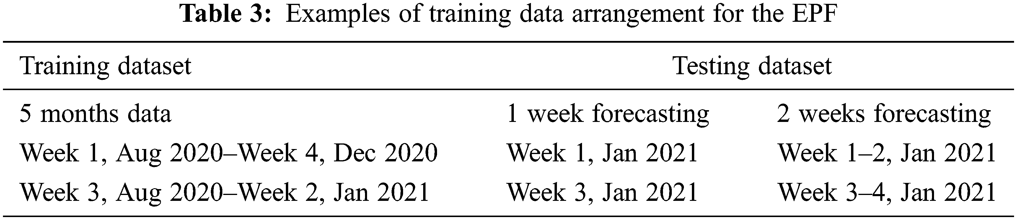
In this work, electricity demand and price data were obtained from Australian Energy Market Operator (AEMO) from August 2020 to May 2021 to develop the proposed mid-term EPF framework. Test dataset includes the hourly data from January 2021 to May 2021. In the meantime, the training dataset is arranged accordingly where 60% of the data is used as training while the rest 40% is used as validation dataset. The training dataset includes 5 prior months to the forecasting weeks. This work proposed two types of forecasting: 1-week forecasting and 2 weeks forecasting. Tab. 3 briefly shows the sample arrangement of training dataset to forecast electricity price for the month of January and February. The arrangement is modified accordingly to forecast the months of March, April and May 2021.
It is argued that the data points used for developing the forecasting model should be strongly correlated with each other. Hence, the correlation coefficient R of the actual and predicted output of the model is computed to assess the feasibility of implementing BTE model. The purpose of analyzing regression model is to extract significant relationships between the forecast variable of interest and the predictor variables. A perfect forecasting modelling will produce a correlation coefficient R value of 1. Figs. 2–6 showed a regression value, R of 0.78, 0.80, 0.88, 0.76, and 0.87 for Australia’s five economic states (NSW, QLD, SA, TAS, VIC) respectively when applying BTE model. As can be seen, the regression value obtained when implementing conventional BTE model is in the range between 0.76 to 0.87 which is inadequate in forecasting complex time series data. Hence, in order to improve the accuracy of the forecasting model, the data was further transferred to RNN model and this work proposed to incorporate GRU in the RNN architecture for further optimization.
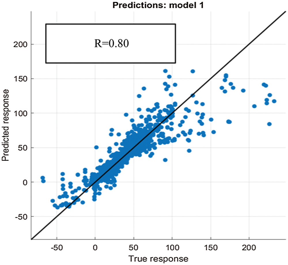
Figure 3: QLD BTE testing model
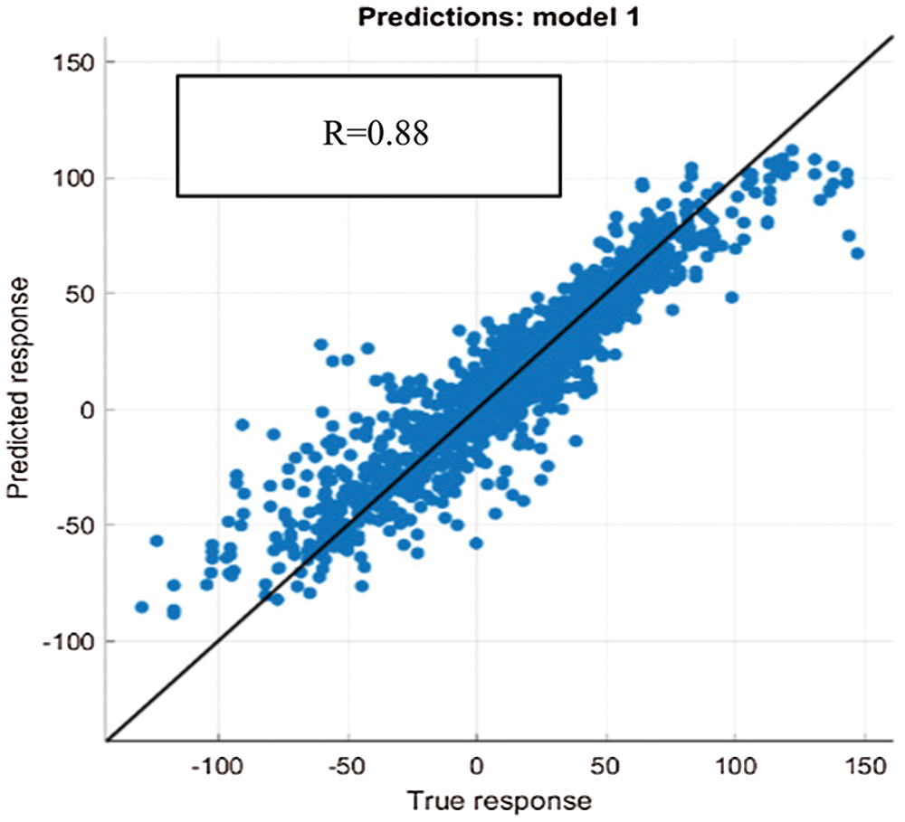
Figure 4: SA BTE testing model
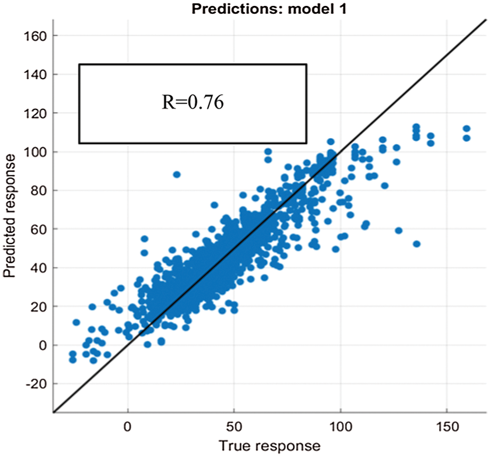
Figure 5: TAS BTE testing model

Figure 6: VIC BTE testing model
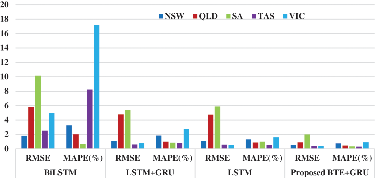
Figure 7: The RMSE and MAPE for EFP using several deep learning methods
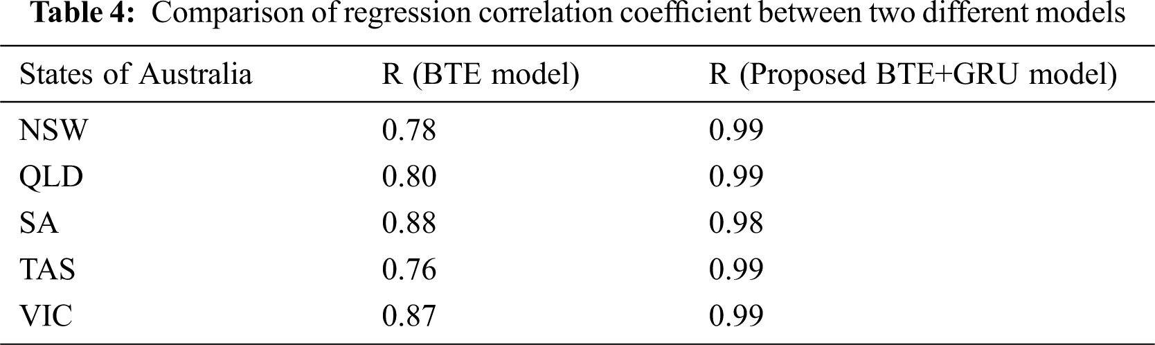
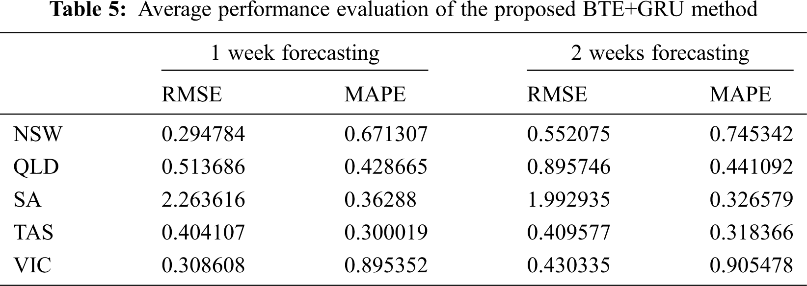
The two weeks forecasting results are compared in Fig. 7. After applying the proposed BTE and GRU model, the correlation coefficient of R for NSW, QLD, SA, TAS, VIC has improved significantly to 0.9961, 0.9995, 0.9800, 0.9996, 0.9996 respectively (Tab. 4). This shows that the proposed forecasting model achieved a correlation coefficient, R approximately 1 which means that the proposed forecasting model manage to correlate the data points better as compared to BTE model in Figs. 2–6. Thus, high value of R contributed to better performance in mean absolute percentage error (MAPE) and root mean square error (RMSE). In this work, the accuracy of the proposed point forecasting model is evaluated by computing the MAPE and RMSE. RMSE evaluates the forecasting precision and the ability of the point prediction results while MAPE conveys the absolute average forecasting deviation of trains and targets. As can be seen from Fig. 7, the proposed BTE+GRU produced the smallest value of RMSE and MAPE values compared to other methods such as BiLSTM, LSTM+GRU, and LSTM for all the five states, NSW, QLD, SA, TAS, VIC. It can be concluded that the most effective method in forecasting the electricity price in this work is the proposed BTE+GRU model where BTE and GRU are incorporated in the RNN architecture. Meanwhile, Tab. 5 tabulated the average performance evaluation of the proposed BTE+GRU method for 1 week and 2 weeks forecasting. The results show that the RMSE and MAPE values are about the same for both types of forecasting interval which means that the forecasting model is feasible to solve 1 week and 2 weeks forecasting problem. Eventually, accurate information on the electricity price forecasting will contribute to effective management in the deregulated electricity market, complex renewable energy and emission policy objectives.

Figure 8: One week forecasting model for NSW
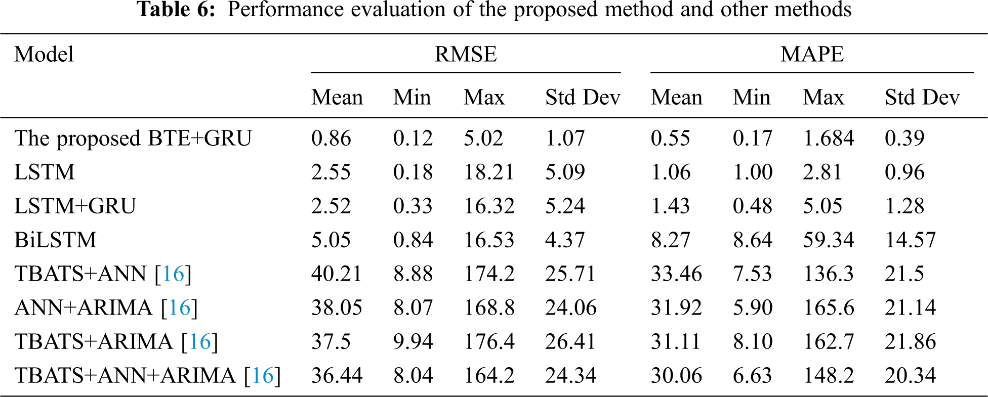
As tabulated in Tab. 6, the proposed model is benchmarked with several methods to measure the effectiveness of the proposed BTE and GRU model. As can be seen, the proposed BTE and GRU model produced the lowest mean RMSE and mean MAPE values as compared to other methods which are 0.86 and 0.55 respectively. The work in [16] adopted machine learning approach with Trend and Seasonal Components (TBATS) which adopted trigonometric technique supports forecasting of daily seasonality by applying maximum likelihood estimation. However, TBATS method does not permit the adoption of external regressors. The computation of TBATS+ANN, ANN+ARIMA, TBATS+ARIMA, TBATS+ANN+ARIMA methods were reported in [16] by using Denmark electricity market. It can be seen that the average RMSE for the four methods applied in [16] is significantly high compared to methods applied in this work that adopted deep learning methods such as LSTM, LSTM+GRU, BiLSTM and the proposed model. This justifies the importance of adopting deep learning method in developing an accurate forecasting model.
Figs. 8 and 9 show the examples of 1-week forecasting results while Figs. 10 and 11 show the examples of 2-week forecasting results when using the proposed model for two different states in Australia. It can be seen that the electricity price fluctuations for different states of Australia differ due to different demand, supply and energy resources. The results justified that the proposed forecasting model can generate comparatively accurate forecasting results and the deviation between the curve of the proposed BTE+GRU model and the actual load curve is considered the lowest compared to other methods as tabulated in Tab. 6.
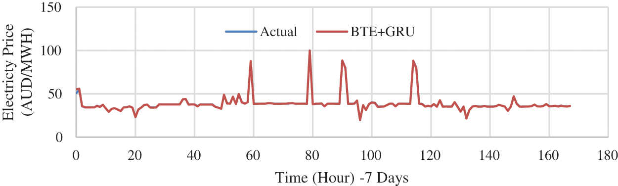
Figure 9: One week forecasting model for TAS
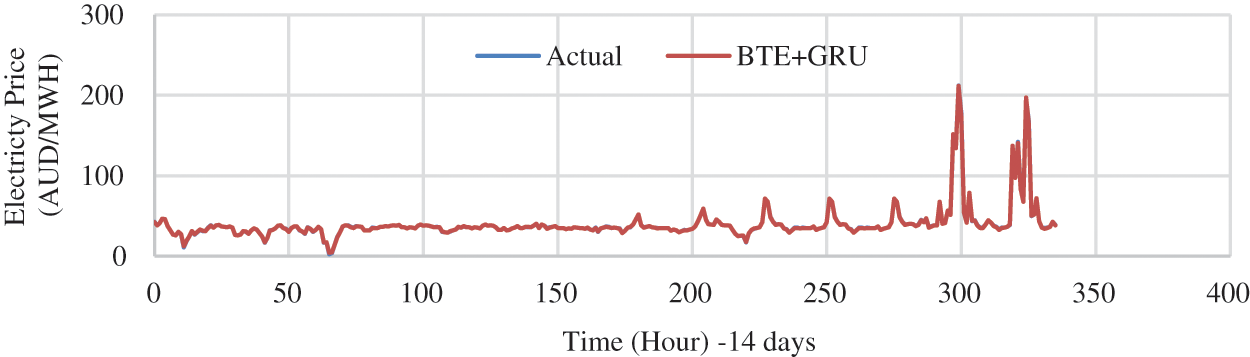
Figure 10: Two weeks forecasting model for NSW
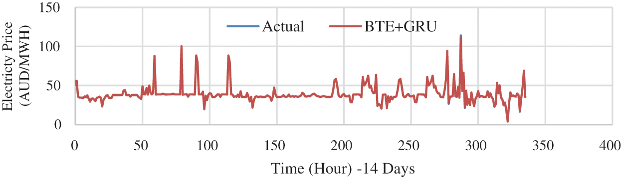
Figure 11: Two weeks forecasting model for TAS
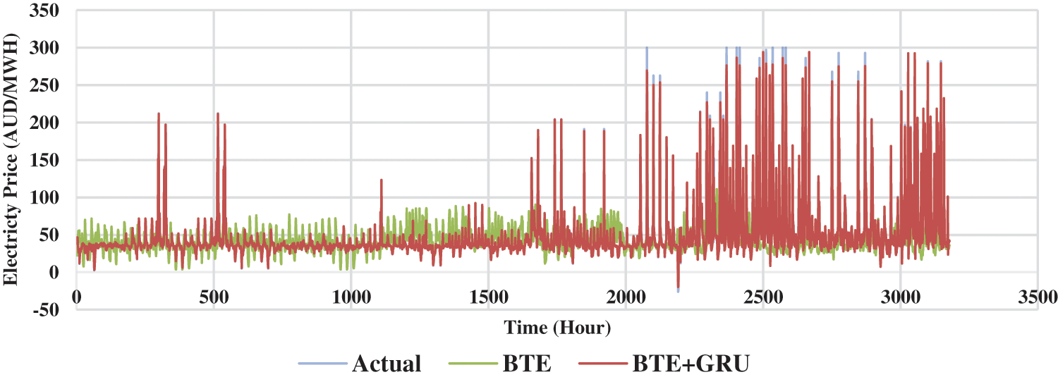
Figure 12: Forecasting model comparison for NSW
Figs. 12–14 presents the 2 weeks forecasting results from the month of January to May 2021 in an hourly basis for three economical states in Australia such as New South Wales, Tasmania and Victoria. At most points, the conventional BTE model was not able to forecast the spikes which justifies the inadequacy of implementing conventional BTE method in EPF. Despite the complex nonlinearity in the trend of electricity price, the proposed model which incorporated BTE and GRU managed to forecast the spikes more accurately and seems to fit the actual data to a satisfactory degree. Hence, this justified the contribution of the proposed model in solving mid-term EPF problem.
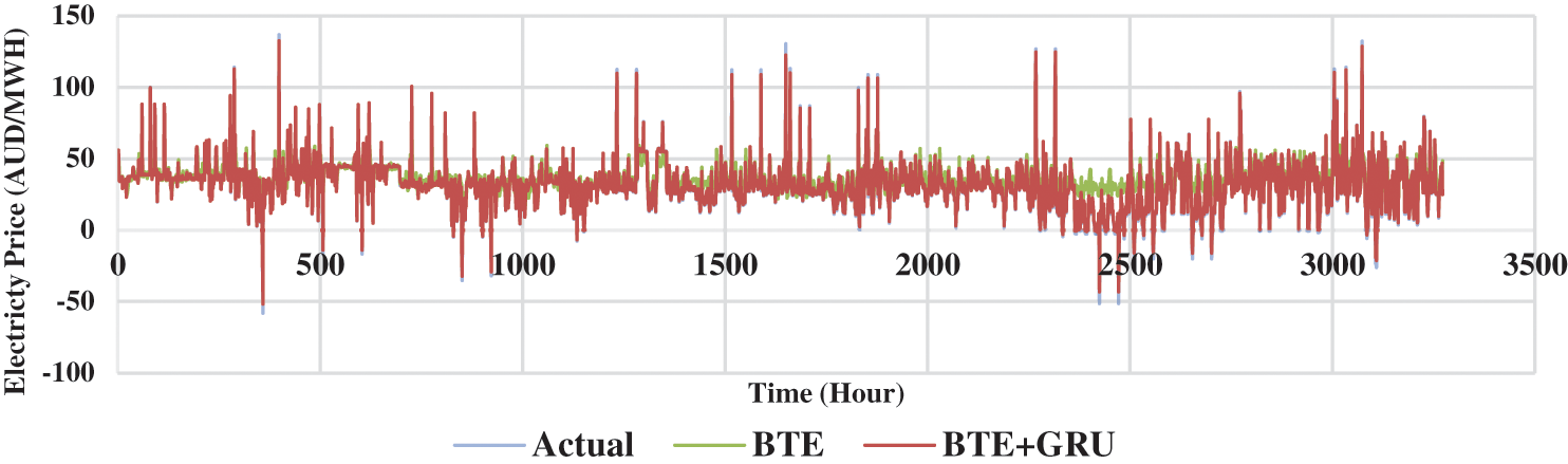
Figure 13: Forecasting model comparison for TAS
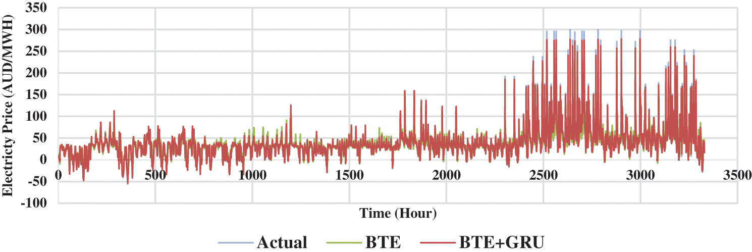
Figure 14: Forecasting model comparison for VIC
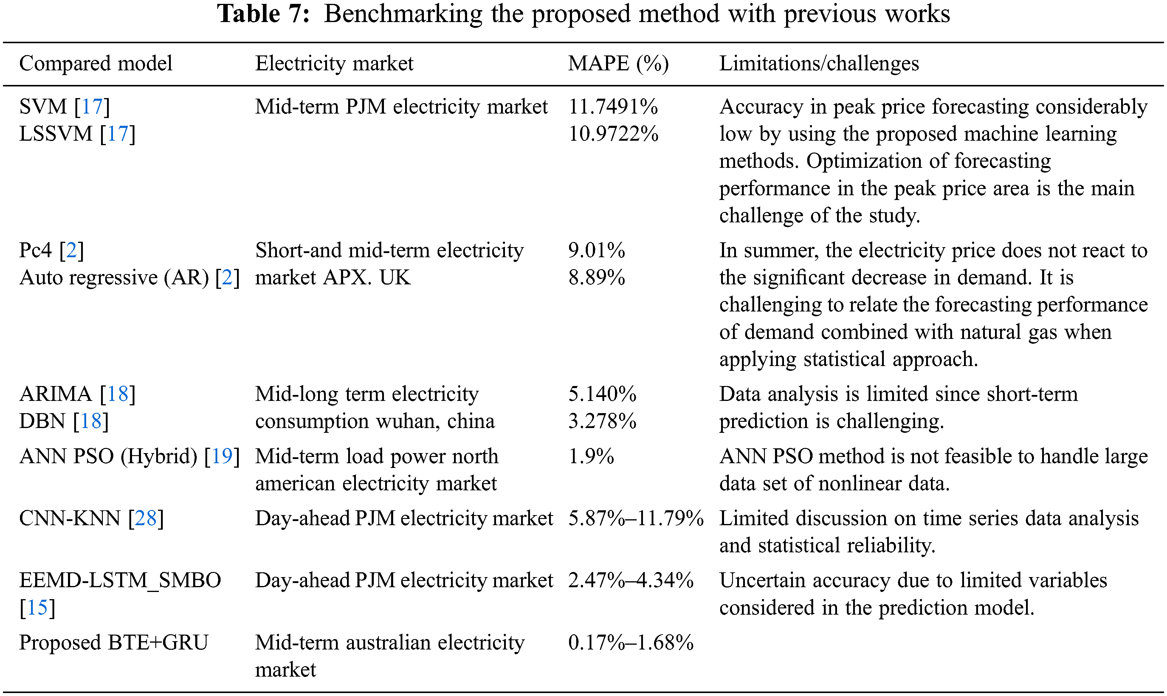
Moreover, the MAPE of the proposed forecasting model is benchmarked with previous works that adopted different electricity market as shown in Tab. 7. It can be summarized that the proposed forecasting model for Australian electricity market is feasible with MAPE value in the range of 0.17% to 1.68% as compared to previous works with MAPE values of approximately 11% in [17], 9% in [2], 3% to 5% in [18], 1.9% in [19], 5.85% to 11.8% in [28], and 2.4% to 4.3% in [15]. The MAPE value was computed by averaging the MAPE values for the five states of Australia that are focused in this work. This suggests that the proposed forecasting model is feasible for multi-regional mid-term electricity price forecasting.
The proposed framework is developed based on information of the demand and price data from various states in Australia (NSW, QLD, SA, TAS, VIC). Furthermore, we also considered renewable and non-renewable energy supplies data, the seasonality, peak and off-peak hours of working and non-working as the forecasting inputs which substantially impact the electricity pricing. In this work, an optimized GRU consisting of RNN with Bagged Regression Tree forecasting model is proposed for electricity price prediction. Then, the tanh layer is employed to optimize the hyperparameters of the heterogeneous GRU with the aim to improve the model’s performance, error reduction and predict the spikes. A machine-learning approach called bagged trees ensemble (BTE) and deep neural network named GRU were successfully integrated in this work to forecast the mid-term electricity price in the current deregulated electricity market. The bagged trees regression is applied to predict nonlinear data which is further optimized by using GRU RNN network. The applied ensemble algorithm managed to enhance the stability of base learners by aggregating the outputs of base learners to generate a single prediction. Finally, a comparative study with conventional time-series models has demonstrated the effectiveness of the proposed methodology. The proposed forecasting model was also compared with previous works and had shown promising results. For future work, the proposed forecasting model can be improved by considering new profit and return-based quality measures. Besides that, the forecasting model can be further modified to solve long-term electricity price forecasting as well. It is worth noting that the methodology presented here can easily be expanded to include a broader scientific domain of time series forecasting applications, such as weather forecasting, earthquake prediction, and heartbeat rate prediction.
Funding Statement: This work is funded by Universiti Malaya research grant from Malaysia under the project name ‘Intelligent Price Forecasting System for Optimal Energy Market’ with grant number ST005-2021. The principal investigator of the research grant is Dr Anis Salwa Mohd Khairuddin while the co-researcher of this grant is Prof. Ir. Dr Hazlie Mokhlis.
Conflicts of Interest: The authors declare that they have no conflicts of interest to report regarding the present study.
1. D. W. Bunn, “Forecasting loads and prices in competitive power markets,” in Proc. of the IEEE, vol. 88, no. 2, pp. 163–169, 2000. [Google Scholar]
2. K. Maciejowska and R. Weron, “Short-and mid-term forecasting of baseload electricity prices in the UK: The impact of intra-day price relationships and market fundamentals,” IEEE Transactions on Power Systems, vol. 31, pp. 994–1005, 2015. [Google Scholar]
3. X. Li, P. Wu and W. Wang, “Incorporating stock prices and news sentiments for stock market prediction: A case of Hong Kong,” Information Processing & Management, vol. 57, pp. 102212, 2020. [Google Scholar]
4. J. Qian, M. Zhu, Y. Zhao and X. He, “Short-term wind speed prediction with a two-layer attention-based LSTM,” Computer Systems Science and Engineering, vol. 39, no. 2, pp. 197–209, 2021. [Google Scholar]
5. S. Borovkova and I. Tsiamas, “An ensemble of LSTM neural networks for high-frequency stock market classification,” Journal of Forecasting, vol. 38, pp. 600–619, 2019. [Google Scholar]
6. G. Sun, J. Lin, C. Yang, X. Yin, Z. Li et al., “Stock price forecasting: An echo state network approach,” Computer Systems Science and Engineering, vol. 36, no. 3, pp. 509–520, 2021. [Google Scholar]
7. P. H. Vuong, T. T. Dat, T. K. Mai, P. H. Uyen and P. T. Bao, “Stock-price forecasting based on XGBoost and LSTM,” Computer Systems Science and Engineering, vol. 40, no. 1, pp. 237–246, 2021. [Google Scholar]
8. N. Amjady, “Short-term hourly load forecasting using time-series modeling with peak load estimation capability,” IEEE Transactions on Power Systems, vol. 16, pp. 498–505, 2001. [Google Scholar]
9. S. S. Pappas, L. Ekonomou, D. C. Karamousantas, G. Chatzarakis, S. Katsikas et al., “Electricity demand loads modeling using AutoRegressive moving average (ARMA) models,” Energy, vol. 33, pp. 1353–1360, 2008. [Google Scholar]
10. A. Pourdaryaei, H. Mokhlis, H. A. Illias, S. H. A. Kaboli, S. Ahmad et al., “Hybrid ANN and artificial cooperative search algorithm to forecast short-term electricity price in de-regulated electricity market,” IEEE Access, vol. 7, pp. 125369–125386, 2019. [Google Scholar]
11. Y. Y. Hong, J. V. Taylar and A. C. Fajardo, “Locational marginal price forecasting using deep learning network optimized by mapping-based genetic algorithm,” IEEE Access, vol. 8, pp. 91975–91988, 2020. [Google Scholar]
12. A. Ciarreta, P. Muniain and A. Zarraga, “Modeling and forecasting realized volatility in German–Austrian continuous intraday electricity prices,” Journal of Forecasting, vol. 36, pp. 680–690, 2017. [Google Scholar]
13. F. Wu, C. Cattani, W. Song and E. Zio, “Fractional ARIMA with an improved cuckoo search optimization for the efficient short-term power load forecasting,” Alexandria Engineering Journal, vol. 59, pp. 3111–3118, 2020. [Google Scholar]
14. E. Kraft, D. Keles and W. Fichtner, “Modeling of frequency containment reserve prices with econometrics and artificial intelligence,” Journal of Forecasting, vol. 39, pp. 1179–1197, 2020. [Google Scholar]
15. S. Zhou, L. Zhou, M. Mao, H. M. Tai and Y. Wan, “An optimized heterogeneous structure LSTM network for electricity price forecasting,” IEEE Access, vol. 7, pp. 108161–108173, 2019. [Google Scholar]
16. O. A. Karabiber and G. Xydis, “Electricity price forecasting in the danish day-ahead market using the TBATS, ANN and ARIMA methods,” Energies, vol. 12, pp. 928, 2019. [Google Scholar]
17. X. Yan, Y. Song and N. A. Chowdhury, “Performance evaluation of single SVM and LSSVM based forecasting models using price zones analysis,” in 2016 IEEE PES Asia-Pacific Power and Energy Engineering Conf. (APPEEC), Xi’an, China, pp. 79–83, 2016. [Google Scholar]
18. C. Hu, H. Yuan, J. J. Zhang, J. Yan, T. Gao et al., “Mid-long term electricity consumption forecasting analysis based on cyber-physical-social system architecture,” in 2020 IEEE 16th Int. Conf. on Automation Science and Engineering (CASE), Hong Kong, China, pp. 564–569, 2020. [Google Scholar]
19. A. Heydari, F. Keynia, D. A. Garcia and L. De Santoli, “Mid-term load power forecasting considering environment emission using a hybrid intelligent approach,” in 2018 5th Int. Symposium on Environment-Friendly Energies and Applications (EFEA), Rome, Italy, pp. 1–5, 2018. [Google Scholar]
20. N. Singh, S. R. Mohanty and R. D. Shukla, “Short term electricity price forecast based on environmentally adapted generalized neuron,” Energy, vol. 125, pp. 127–139, 2017. [Google Scholar]
21. A. Ntakaris, M. Magris, J. Kanniainen, M. Gabbouj and A. Iosifidis, “Benchmark dataset for mid-price forecasting of limit order book data with machine learning methods,” Journal of Forecasting, vol. 37, pp. 852–866, 2018. [Google Scholar]
22. J. Dhillon, S. A. Rahman, S. U. Ahmad and M. J. Hossain, “Peak electricity load forecasting using online support vector regression,” in 2016 IEEE Canadian Conf. on Electrical and Computer Engineering (CCECE), pp. 1–4, 2016. [Google Scholar]
23. E. E. Elattar, S. K. Elsayed and T. A. Farrag, “Hybrid local general regression neural network and harmony search algorithm for electricity price forecasting,” IEEE Access, vol. 9, pp. 2044–2054, 2020. [Google Scholar]
24. Y. Chen, P. Xu, Y. Chu, W. Li, Y. Wu et al., “Short-term electrical load forecasting using the support vector regression (SVR) model to calculate the demand response baseline for office buildings,” Applied Energy, vol. 195, pp. 659–670, 2017. [Google Scholar]
25. L. Wang, S. X. Lv and Y. R. Zeng, “Effective sparse adaboost method with ESN and FOA for industrial electricity consumption forecasting in China,” Energy, vol. 155, pp. 1013–1031, 2018. [Google Scholar]
26. J. Wu, Z. Cui, Y. Chen, D. Kong and Y. G. Wang, “A new hybrid model to predict the electrical load in five states of Australia,” Energy, vol. 166, pp. 598–609, 2019. [Google Scholar]
27. A. Pourdaryaei, H. Mokhlis, H. A. Illias, S. H. A. Kaboli and S. Ahmad, “Short-term electricity price forecasting via hybrid backtracking search algorithm and ANFIS approach,” IEEE Access, vol. 7, pp. 77674–77691, 2019. [Google Scholar]
28. R. Zhang, G. Li and Z. Ma, “A deep learning based hybrid framework for day-ahead electricity price forecasting,” IEEE Access, vol. 8, pp. 143423–143436, 2020. [Google Scholar]
29. H. Manner, F. A. Fard, A. Pourkhanali and L. Tafakori, “Forecasting the joint distribution of Australian electricity prices using dynamic vine copulae,” Energy Economics, vol. 78, pp. 143–164, 2019. [Google Scholar]
30. H. Wang, Q. Xu and L. Zhou, “Large unbalanced credit scoring using lasso-logistic regression ensemble,” PloS One, vol. 10, pp. e0117844, 2015. [Google Scholar]
31. V. B. Nguyen, M. T. Duong and M. H. Le, “Electricity demand forecasting for smart grid based on deep learning approach,” in 2020 5th Int. Conf. on Green Technology and Sustainable Development (GTSD), Ho Chi Minh City, Vietnam, pp. 353–357, 2020. [Google Scholar]
32. A. Tokgöz and G. Ünal, “A RNN based time series approach for forecasting turkish electricity load,” in 2018 26th Signal Processing and Communications Applications Conf. (SIU), Izmir, Turkey, pp. 1–4, 2018. [Google Scholar]
33. M. Pan, H. Zhou, J. Cao, Y. Liu, J. Hao et al., “Water level prediction model based on GRU and CNN,” IEEE Access, vol. 8, pp. 60090–60100, 2020. [Google Scholar]
34. F. M. Shakiba and M. Zhou, “Novel analog implementation of a hyperbolic tangent neuron in artificial neural networks,” IEEE Transactions on Industrial Electronics, vol. 68, no. 11, pp. 10856–10867, 2020. [Google Scholar]
35. J. Manotumruksa, C. Macdonald and I. Ounis, “A contextual recurrent collaborative filtering framework for modelling sequences of venue checkins,” Information Processing & Management, vol. 57, pp. 102092, 2020. [Google Scholar]
36. Y. Yu, K. Adu, N. Tashi, P. Anokye, X. Wang et al., “Rmaf: Relu-memristor-like activation function for deep learning,” IEEE Access, vol. 8, pp. 72727–72741, 2020. [Google Scholar]
 | This work is licensed under a Creative Commons Attribution 4.0 International License, which permits unrestricted use, distribution, and reproduction in any medium, provided the original work is properly cited. |