Computer Systems Science & Engineering DOI:10.32604/csse.2022.024239
Article

Pattern Recognition of Modulation Signal Classification Using Deep Neural Networks

D. Venugopal1, V. Mohan2, S. Ramesh3, S. Janupriya4, Sangsoon Lim5,* and Seifedine Kadry6

1Department of Electronics and Communication Engineering, KPR Institute of Engineering and Technology, Coimbatore, 641048, India
2Department of Electronics and Communication Engineering, Saranathan College of Engineering, Trichy, 620012, India
3Department of Computer Science and Engineering, Krishnasamy College of Engineering & Technology, Cuddalore, 607109, India
4Department of Electronics and Communication Engineering, K. Ramakrishnan College of Engineering, Tiruchirappalli, 621112, India
5Department of Computer Engineering, Sungkyul University, Anyang, Korea
6Department of Applied Data Science, Noroff University College, Kristiansand, Norway
*Corresponding Author: Sangsoon Lim. Email: lssgood80@gmail.com
Received: 10 October 2021; Accepted: 11 November 2021

Abstract: In recent times, pattern recognition of communication modulation signals has gained significant attention in several application areas such as military, civilian field, etc. It becomes essential to design a safe and robust feature extraction (FE) approach to efficiently identify the various signal modulation types in a complex platform. Several works have derived new techniques to extract the feature parameters namely instant features, fractal features, and so on. In addition, machine learning (ML) and deep learning (DL) approaches can be commonly employed for modulation signal classification. In this view, this paper designs pattern recognition of communication signal modulation using fractal features with deep neural networks (CSM-FFDNN). The goal of the CSM-FFDNN model is to classify the different types of digitally modulated signals. The proposed CSM-FFDNN model involves two major processes namely FE and classification. The proposed model uses Sevcik Fractal Dimension (SFD) technique to extract the fractal features from the digital modulated signals. Besides, the extracted features are fed into the DNN model for modulation signal classification. To improve the classification performance of the DNN model, a barnacles mating optimizer (BMO) is used for the hyperparameter tuning of the DNN model in such a way that the DNN performance can be raised. A wide range of simulations takes place to highlight the enhanced performance of the CSM-FFDNN model. The experimental outcomes pointed out the superior recognition rate of the CSM-FFDNN model over the recent state of art methods interms of different evaluation parameters.

Keywords: Pattern recognition; signal modulation; communication signals; deep learning; feature extraction

1  Introduction

For classical pattern recognition problems, the modulation identification of transmission signals has several application values and significant study prospects. In the military fields, it is a pre-condition for performing transmission jamming and reconnaissance. When the signal modulation of the enemies’ transmission scheme is simplified, the enemy’s signal could be demodulated and data transmission could be attained. In the civil field, signal modulation identification could be utilized for interference identification, signal confirmation, spectrum monitoring, and spectrum management. Thus, reliable and secure feature extraction (FE) methods are required for efficiently recognizing the distinct signal modulations [1] in a complicated situation.

Now, Automatic modulation classification (AMC) was a conventional area of research. AMC recognizes the modulation kind of the transferred signal manually. It performs an important part in developing smart transmission schemes such as radio spectrum and cognitive radios monitoring [2]. It could be viewed that the receivers consist of an automated modulation classifier i.e., additionally divided into 2 major submodules: classifier module and received signal preprocessing correspondingly [3]. The preprocessing blocks are tasked with estimating the synchronization parameters such as timing recovery, power received signals frequency offset, and so on. Alternatively, the classifiers module selects a sufficient classification approach for the modulations identification. In this study, AMC is classified into 2 major classes: 1) Feature based and 2) Likelihood based [4]. In both classes, the obtained signal instances are related to a pool having feasible modulation candidate denoted as M (i), in which i represented the amount of modulation candidates in the pool.

Hood based AMC determines likelihood ratio of obtained signal and relates to a threshold for getting possible modulation candidates. The feature related approaches treat AMC as a pattern detection challenge [5]. It determines the different features from the obtained signals and classifications are executed according to the analyzed value of this feature. Likelihood based approaches give and best solution to AMC problems however it comes at the cost of significant computation complexity [6]. Alternatively, the feature based approaches provide a nearby optimum efficiency with lower complexity and thus are generally applied in real-world executions. Actually, the feature based approaches employ 2 major subsystems: 1) Classification, 2) FE. Several features were utilized in prior studies for modulation recognition. Wavelet transforms Higher order cumulant, multi cumulant, and signal spectral related features are few characteristics i.e., presented in the study for supervised classifications. Conversely, few unsupervised clustering based approaches were introduced for AMC [7]. It considers the merits of the constellation diagrams of the obtained modulation candidates and hence it doesn’t need the group labels to train the classifiers.

The deep learning (DL) approach is capable of extracting the fundamental features and incorporate them for obtaining high level features. Afterward, including classifications of features, the feature distribution characteristic of the targeted objects could be examined [8]. Furthermore, this method has a stronger capability of fitting the features of data (Hossain et al., (2019)). Recently, various researches have displayed that machine learning (ML) technique could be employed for signal pattern recognition/signal FE, however, the actual application procedure would be influenced by the variation of SNR [9]. The detection of modulation signal using DL approach has higher strength, and also the detection kinds are highly complex. However, in the real-world application, it would be complex for realizing due to the difficulty of the approach [10]. Hence, it has high importance for constructing a modulation signal pattern detection method with large dynamic and good generalization SNR. But, it is the greatest issue for manually recognizing the characteristics parameter, the modulation, and recognition technique of the classifiers in the modulation signal efficiently, and employ the detection of modulation signal patterns.

This paper designs pattern recognition of communication signal modulation using fractal features with deep neural networks (CSM-FFDNN) to classify the different types of digitally modulated signals (such as Amplitude Shift Keying (ASK, M = 2, 4), Frequency Shift Keying (FSK, M = 2, 4, 8), Multiple Phase Shift Keying (BPSK), 16QAM (Quadrature Amplitude Modulation), and 32QAM. The proposed CSM-FFDNN model uses Sevcik Fractal Dimension (SFD) technique to extract the fractal features from the digital modulated signals. Besides, the extracted features are fed into the DNN model for modulation signal classification. To boost the classifier results of the DNN model, a barnacles mating optimizer (BMO) is used for the hyperparameter tuning of the DNN model in such a way that the DNN performance can be raised. A comprehensive experimental analysis is made to point out the improved outcomes of the CSM-FFDNN model.

2  Related Works

Shi [11] proposed a systematic analysis with the help of fractal dimensions as the features of modulation signal. Katz, Box, Petrosian, Sevcik, and Higuchi fractal dimensions, are extracted from 8 distinct modulation signals for recognizing signals pattern. While, the running time, antinoise function, and box diagrams are utilized for evaluating the separability, computation complexity, and noise robustness of 5 distinct fractal features. Lastly, grey relation analysis, BPNN, RF, and KNN are presented for classifying distinct modulation signals according to this fractal feature. Ali et al. [12] investigate the use of DNN to the automated categorization of modulation signals in AWGN and flat fading channels. The 3 training inputs are utilized; generally 1) the centroid of constellation point employs the fuzzy C-mean approach to I-Q diagram, 2) the higher order cumulant of attained instance, and 3) quadrature (I-Q) and In-phase constellation point. The unsupervised learning from this dataset was made by the sparse AE and a supervised soft-max classifier has been applied to the classification.

Zhou et al. [13], proposed a robust AMC technique with CNN approach. Generally, fifteen distinct modulation kinds are taken into account. The presented technique could categorize the obtained signal straightaway with no FE approach, and it could manually acquire features from the obtained signal. The feature learned using the CNNs are analyzed and presented. The robust feature of obtained signals in certain SNR ranges are examined. The classification performance with CNN is displayed to be outstanding, mainly for lower SNR. Also, the generalization capability of robust features is shown to be remarkable utilizing SVM algorithm.

Zhang et al. [14] proposed a mixed recognition approach according to 2 novel and another traditional feature, and develop tree shaped multilayer SSVM classifiers on the basis of FS approach for recognizing 7 types of digital modulation signals. In Wang, et al. [15], a new DL based LightAMC approach is presented using small model size and fast computation speed. First, they present scaling factors for all neurons in CNN and enforces scaling factor sparsity. It could provide support to discard the repetitive neurons.

Hong et al. [16] proposed a new AMC approach on the basis of RNN approach, i.e., displayed to have the ability to adequately exploiting the temporal sequence characteristics of attained transmission signal. This technique resorts to raw signal directly by constrained data length and manually evades extracting signal features. The presented technique is related to CNN based methods and the results indicate the superiority of the presented approach. Wang et al. [17] presented a CNN based Co-AMC technique for the MIMO system, in which the recipient, armed with multiple antennas, co-operatively identifies the modulation type. Especially, every receiving antenna give their detection sub results through the CNN, correspondingly. Next, the decision-maker recognizes the modulation type, according to this sub result and co-operative decision rules.

3  The Proposed Model

Fig. 1 demonstrates the general working process of the CSM-FFDNN technique. In this study, a new CSM-FFDNN model is designed to classify various kinds of digitally modulated signals such as MASK, MFSK, BPSK, and QAM. The proposed CSM-FFDNN model involves three major processes namely fractal FE, DNN based classification, and BMO based hyperparameter optimization. The detailed working of these processes is elaborated in the succeeding sections.

3.1 Fractal Feature Extraction

At this stage, the fractal features from the communication signals are extracted using the SFD technique. Self similar dimension is complicated for employing objects that aren’t severely self similar, and the box dimensions could be utilized for overcoming these challenges. In the metric space (X,d),A is belonging to M non-empty emergency cluster of X . For a box using side length of ϵ , the minimal value N(A,ϵ) of box needed to cover A is given in the following equation [18]:

N(A,ϵ)={M:A⊂∑i=1M⁡N(xi,ϵ)}, (1)

In which x1,x2, ⋯xM represent distinct points of X . While ϵ approaching , the box dimensions are displayed in the following equation:

Db=limϵ→0InN(A,ϵ)In(1/ϵ). (2)

As aforementioned, assuming the signals consist of a sequence of points (xi,yi) , the length of signal is N. first Normalise the signal:

xi∗=xi−xminxmax−xmin,yi∗=yi−minymax−ymin (3)

xmin,ymin represents the minimal values amongst xj,yj. xmax, ymax indicates the maximal values amongst xj,yj. Next, the Sevcik fractal dimension D could be estimated in the following equation:

D=1+ln(L)+ln(2)ln[2×(N−1)], (4)

whereas L represents the length of waveform, given below:

L=∑i=0N−2⁡(yi+1∗−yi∗)2+(xi+1∗−xi∗)2. (5)

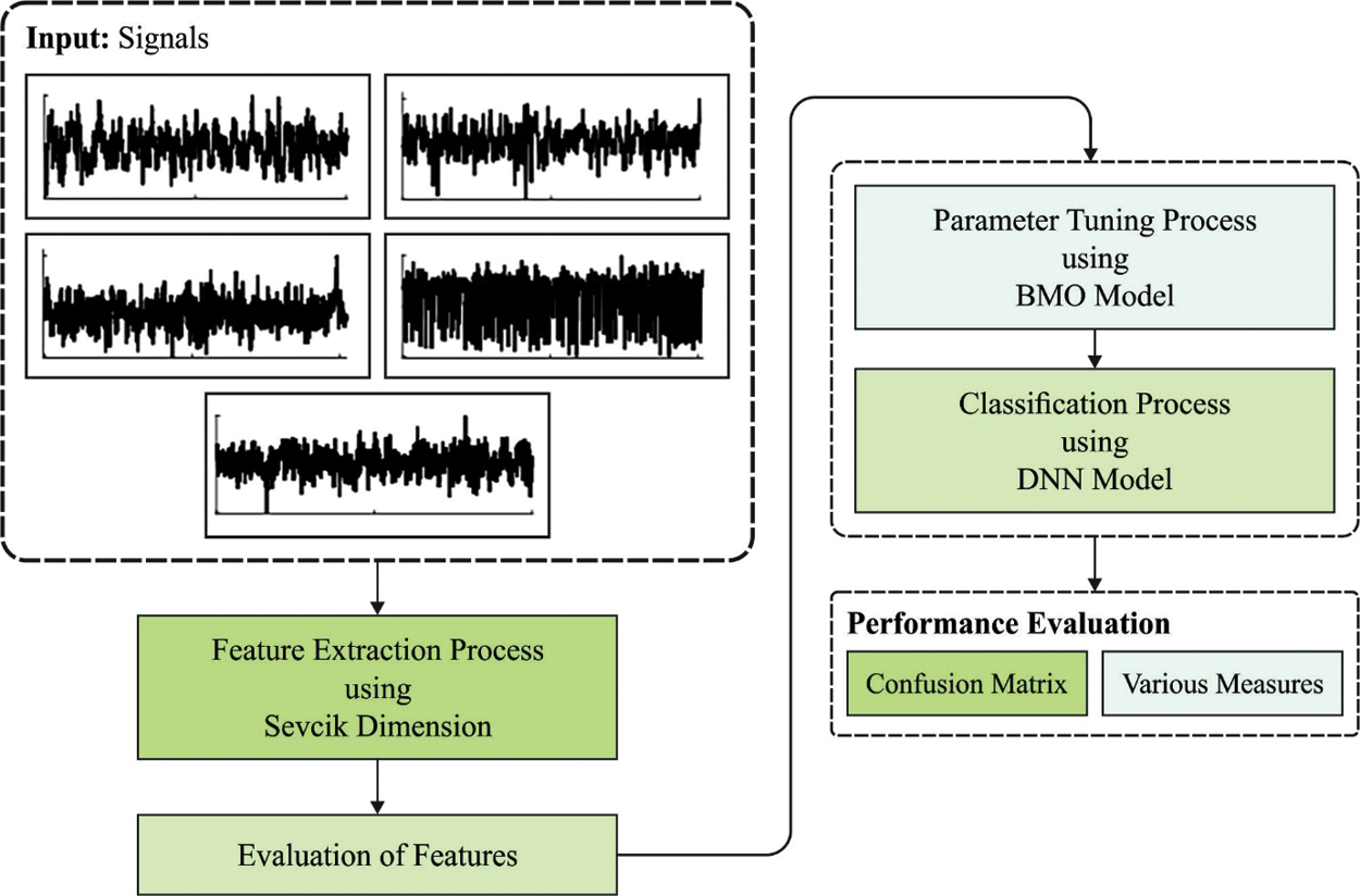
Figure 1: Overall process of CSM-FFDNN model

3.2 Modulation Signal Classification

For the classification of modulation signals, the features are passed into the DNN model. Essentially, the architecture of DNN has 3 main elements that consist of hidden, input, and output layers. The presented framework of DNN is displayed in Fig. 2. Based on the efforts of preference weight fitness, the DNN algorithm is developed using 2 hidden layers (HLs) to effectively learn the mapping relations among the output and input data. In the training stage, with the help of BMO algorithm, the DNN approach iteratively upgrades the node weight in the HL. Because of the increment in the training iteration, this NN repeatedly fits the labeled training data decision boundaries [19]. To boost the classifier results and training speed of DNN, 2 HLs were made. At the HL, the overall number of nodes are calculated in Eq. (6).

n=a+b+c (6)

whereas, the amount of input layer nodes is denoted as a the amount of output layer nodes is provided as b , the amount of HL nodes is given as n and a constant values among [1–10] are represented as c.

In order to enable the nonlinear fitness capability activation functions are included in the HLs of DNN. They have utilized the sigmoid as an activation function and it is represented in the following equation,

S=11+e−x (7)

The input data of networks are called x and it is activated with the mapping function Mf .

Mf=sigm(ωix+βi) (8)

whereas, ω & β signifies the weight matrix and the bias among the output as well as HLs correspondingly.

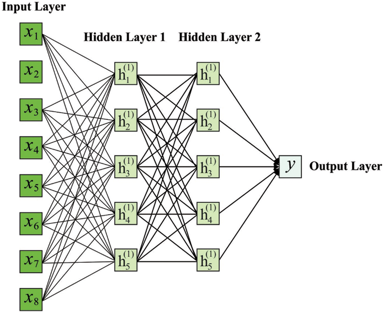
Figure 2: Framework of DNN

In order to create the depiction space of the hidden neuron for aligning with human’s intelligence, they present other supervised loss functions for DNN. In this instance, they need to use the data included in the data instance label that denote the human concept. Assume a conceptual labeled data samples (x,l) for a HL, the loss forms are calculated by

S(Ws,bs;x,l)=12m∑j=1m⁡‖hj(Ws,bs;x)−lj‖22 (9)

In which Ws & bs represents the subset of bias and m indicates the amount of neurons in the HL The utilization of cross entropy loss is highly enhanced by the efficiency of sigmoid and soft-max output models. The cross entropy losses are calculated using Eq. (10).

CE=1n∑k=1n⁡[YklogY^k+(1−Yk)log(1−Y^k)] (10)

Let, n indicates the training instance quantity, Yk represents the kth actual output of training set, Y^k denotes the kth anticipated output of testing set. They are utilizing BMO approach for the optimum weight election of DNN network. In the population enhancing the fitness value of all solutions is the primary objective of BMO algorithm. By upgrading the values, this method effort the fitness value to move toward an optimal solution. Next, the novel solution and the older solution are related and for the upcoming iteration, only an optimal solution is taken into account.

3.3 Hyperparameter Optimization

The BMO algorithm is stimulated by the mating characteristics of barnacles. The procedures contained in the BMO technique are provided here [20].

At the initiation point, it can be regarded as candidate of outcome is barnacle but vector of population is demonstrated as:

X=[x11⋯x1N⋮⋱⋮xn1⋯xnN] (11)

where N represents the amount of adjusting parameters and n illustrates the population size. The control parameter in Eq. (11) has been exposed to upper and lower boundaries of problem that is to be solved as:

llb=[llb1,…,llbi] (12)

lb=[lb1,…,lbi] (13)

where ub and lb are the higher and lower limits of ith variable. The compute of vector X has been whole in the establishment, and the sort procedures are performed to place the optimum result at top of vector X.

The presented BMO technique is executed with this technique to select that is compared with EA techniques as selective of 2 barnacles are dependent upon length of penises pl . The selective model reflects the characteristics of barnacles which depends on given consideration:

i)   The selective procedure was carried out in an arbitrary algorithm; but, it can be restricted to penis length of barnacle pl .

ii)   The selective method selects an identical barnacle which represents self-mating was implemented. The self-mating was extremely arbitrary and barnacle male and female reproductions, therefore, the self-mating has been considered, and a novel off-spring was formed.

iii)   If the selective is dependent upon particular iteration that is superior to pl , the sperm casting was implemented.

The offspring production has been estimated by sperm cast procedure which is determined as the subsequent. It can be manner of this technique that has been performed interms of virtual distance. The provided as easy selective was implemented and it can be written as mathematical procedure:

barnacle−d=randperm(n) (14)

barnacle−m=randperm(n) (15)

where the barnacle_d and barnacle_m are determined as parents that are mated and n represents the population size. Eqs. (14) and (15) demonstrates the selection has been made randomly and fulfills the concern value 1 in the current subsection.

Reproduction

The reproduction process projected in BMO has been compared to EAs. As there are no specific equations to derive the reproduction of barnacles, the BMO has been simplifying on inheritance genotype frequency of barnacle parent’s from creating the offspring depend on Hardy–Weinberg approach. In order to signify the simplicity of presented BMO, the subsequent function has been projected to develop new variables of offspring from barnacle parents:

xiN−new=pxbarnacle−dN+qxbarnacle−mN (16)

where p determined the scattered usually with pseudo random value in 0 and 1 , q=(1−p),xbarnacle−dN and xbarnaclemN are determined as variables of Dad and Mum of barnacles correspondingly. It can be obvious in Eqs. (14) and (15). So, the offspring inherit the nature of Dad as well as Mum dependent upon possibilities of arbitrary values from [0–1]. It could be essential to point a measure of pl that performs an essential one in computing the exploitation and exploration functions. The sperm cast was carried out but the selected barnacles are that exists managed and pl has been assigned initially.

xin−new=rand()×xbarnacle−mn (17)

where rand() implies the arbitrary number amongst 0 and 1 . It can be noted that Eq. (17) illustrates the elegant technique of barnacles offspring. A novel offspring has been formed in Mum barnacle to exploration.

4  Performance Validation

This section has examined the modulation signal classification performance of the proposed model under different dimensions. Tab. 1 and Fig. 3 investigates the fractal features obtained by the Sevcik dimension under varying levels of SNR levels. The results depicted that the Sevcik dimension gets reduced with an increase in SNR values. For instance, with SNR of −5dB, the Sevcik dimension of the 2 ASK, 4 ASK, 2 FSK, 4 FSK, 8 FSK, BPSK, 16 QAM, and 32QAM modulation signals are 1.73, 1.72, 1.73, 1.73, 1.71, 1.75, 1.77, and 1.81 respectively. Along with that, with SNR of −1dB, the Sevcik dimension of the 2 ASK, 4 ASK, 2 FSK, 4 FSK, 8 FSK, BPSK, 16 QAM, and 32QAM modulation signals are 1.68, 1.73, 1.69, 1.66, 1.70, 1.69, 1.78, and 1.80 correspondingly. In the same way, with SNR of 2dB, the Sevcik dimension of the 2 ASK, 4 ASK, 2 FSK, 4 FSK, 8 FSK, BPSK, 16 QAM, and 32QAM modulation signals are 1.65, 1.67, 1.63, 1.63, 1.67, 1.66, 1.77, and 1.81 correspondingly. On continuing with, with SNR of 6dB, the Sevcik dimension of the 2 ASK, 4 ASK, 2 FSK, 4 FSK, 8 FSK, BPSK, 16QAM, and 32QAM modulation signals are 1.63, 1.70, 1.57, 1.59, 1.63, 1.64, 1.75, and 1.79 respectively. Lastly, with SNR of 10dB, the Sevcik dimension of the 2 ASK, 4 ASK, 2 FSK, 4 FSK, 8 FSK, BPSK, 16QAM, and 32QAM modulation signals are 1.59, 1.71, 1.55, 1.60, 1.61, 1.64, 1.77, and 1.78 correspondingly.

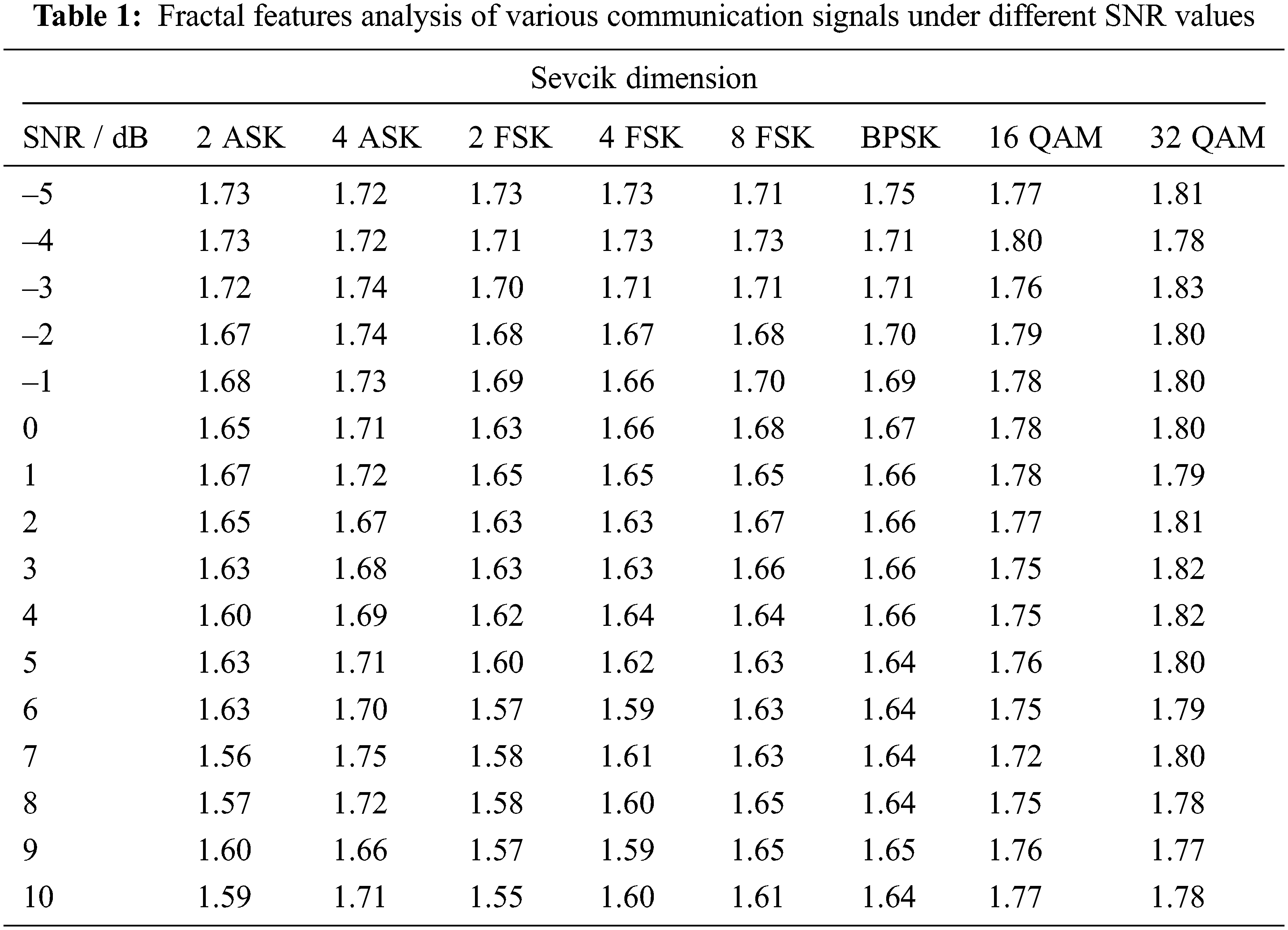
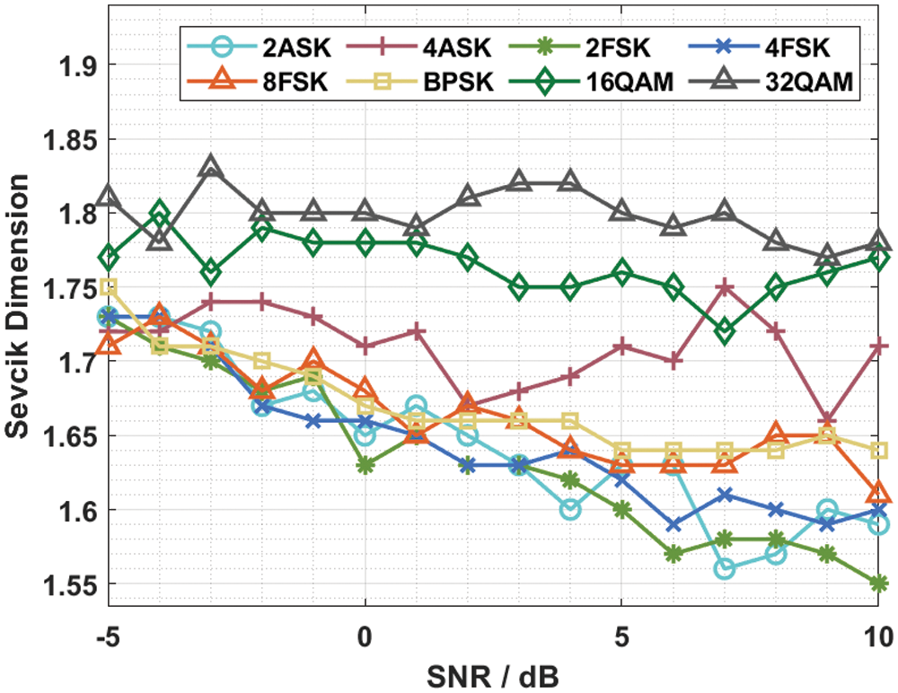
Figure 3: Fractal features of various communication signals

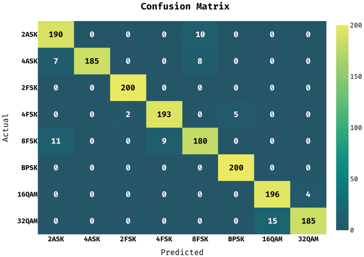
Figure 4: Confusion matrix of DNN model

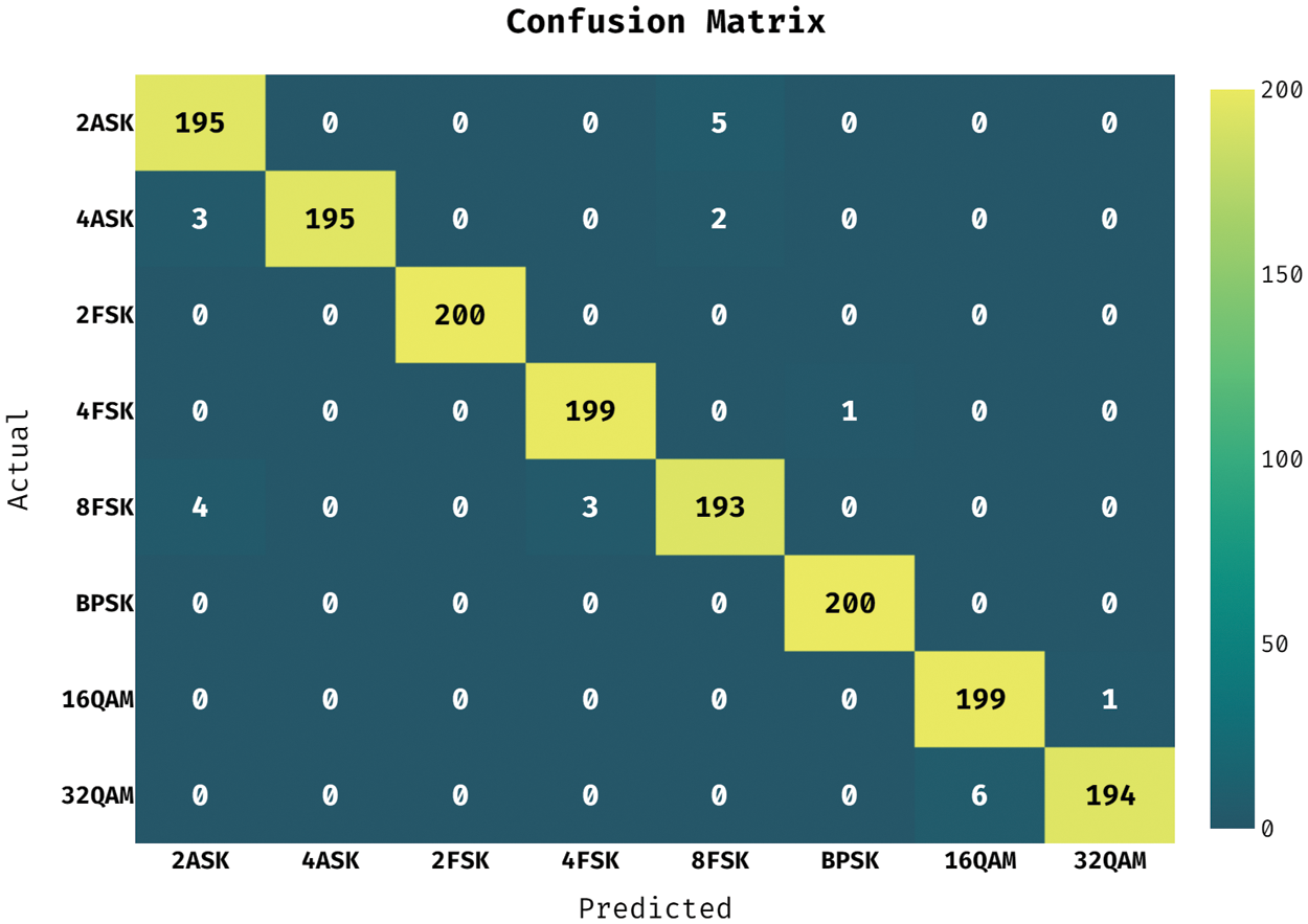
Figure 5: Confusion matrix of BMO-DNN model

Fig. 4 illustrates the confusion matrix produced by the DNN model on the classification of distinct digitally modulated signals. The figure depicted that the DNN model has classified 190 signals into 2ASK, 185 signals into 4ASK, 200 signals into 2FSK, 193 signals into 4 FSK, 180 signals into 8FSK, 200 signals into BPSK, 196 signals into 16QAM, and 185 signals into 32QAM.

Fig. 5 showcases the confusion matrix produced by the BMO-DNN method on the classification of different digitally modulated signals. The figure outperformed that the BMO-DNN approach has classified 195 signals into 2ASK, 195 signals into 4ASK, 200 signals into 2FSK, 199 signals into 4 FSK, 193 signals into 8FSK, 200 signals into BPSK, 199 signals into 16QAM, and 194 signals into 32QAM.

Tab. 2 investigates the performance of the DNN and BMO-DNN techniques under varying modulation types. On the classification of 2ASK signal, the DNN model has obtained a precision of 0.9135, recall of 0.9500, accuracy of 0.9825, and F-score of 0.9314. Likewise, on the classification of 4FSK signal, the DNN method has attained a precision of 0.9554, recall of 0.9650, accuracy of 0.9900, and F-score of 0.9602. Concurrently, on the classification of BPSK signal, the DNN technique has obtained a precision of 0.9756, recall of 1.0000, accuracy of 0.9969, and F-score of 0.9877. Simultaneously, on the classification of 32QAM signal, the DNN manner has achieved a precision of 0.9788, recall of 0.9250, accuracy of 0.9881, and F-score of 0.9512. Also, on the classification of 2ASK signal, the BMO-DNN manner has got a precision of 0.9653, recall of 0.9750, accuracy of 0.9925, and F-score of 0.9701. Besides, on the classification of 4FSK signal, the BMO-DNN method has gained a precision of 0.9851, recall of 0.9950, accuracy of 0.9975, and F-score of 0.9900. Additionally, on the classification of BPSK signal, the BMO-DNN technique has obtained a precision of 0.9950, recall of 1.0000, accuracy of 0.9994, and F-score of 0.9975. Furthermore, on the classification of 32QAM signal, the BMO-DNN methodology has led to a precision of 0.9949, recall of 0.9700, accuracy of 0.9956, and F-score of 0.9823.

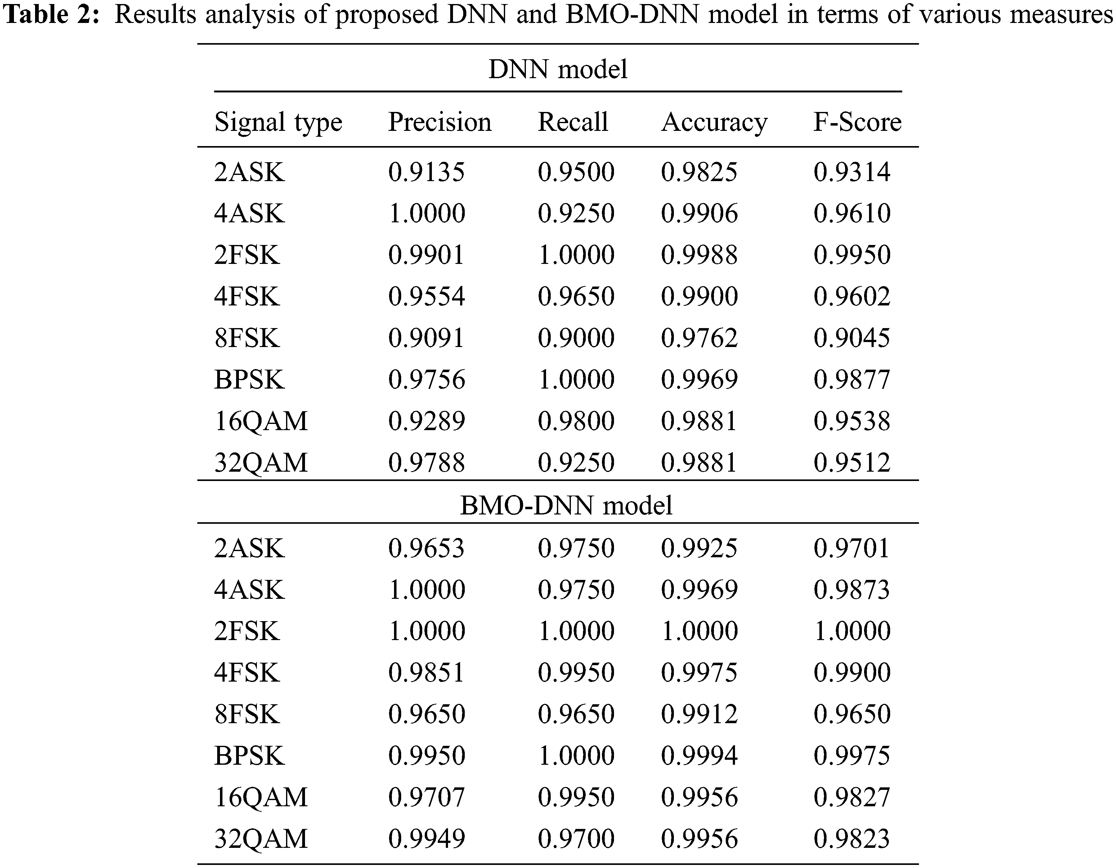
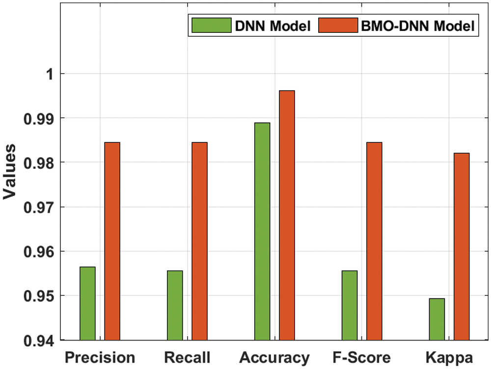
Figure 6: Performance analysis of BMO-DNN technique

An average results analysis of the BMO-DNN technique and DNN technique take place in Fig. 6 and Tab. 3. The table values depicted that the DNN technique has resulted in an average precision of 0.9564, recall of 0.9556, accuracy of 0.9889, F-score of 0.9556, and kappa of 0.9493. Besides, the BMO-DNN technique has obtained better performance with an average precision of 0.9845, recall of 0.9844, accuracy of 0.9961, F-score of 0.9844, and kappa of 0.9821. These values portrayed that the BMO-DNN technique has outperformed the DNN technique.

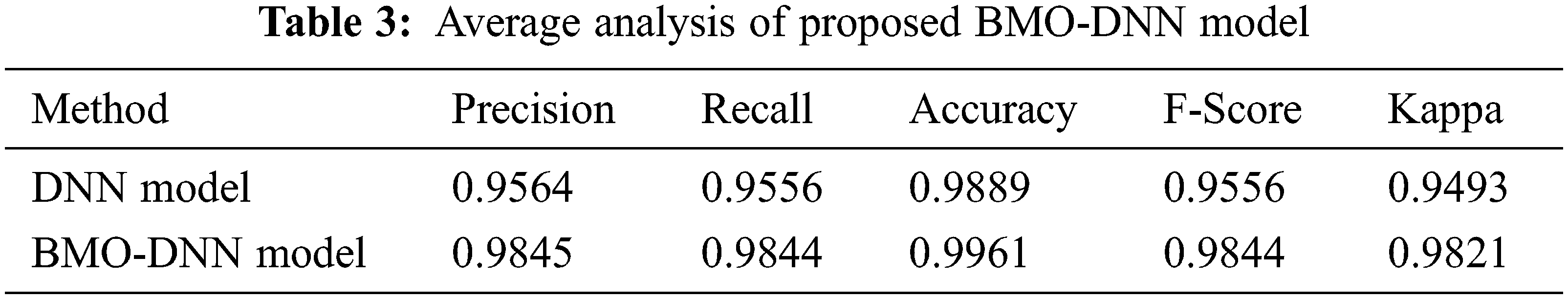
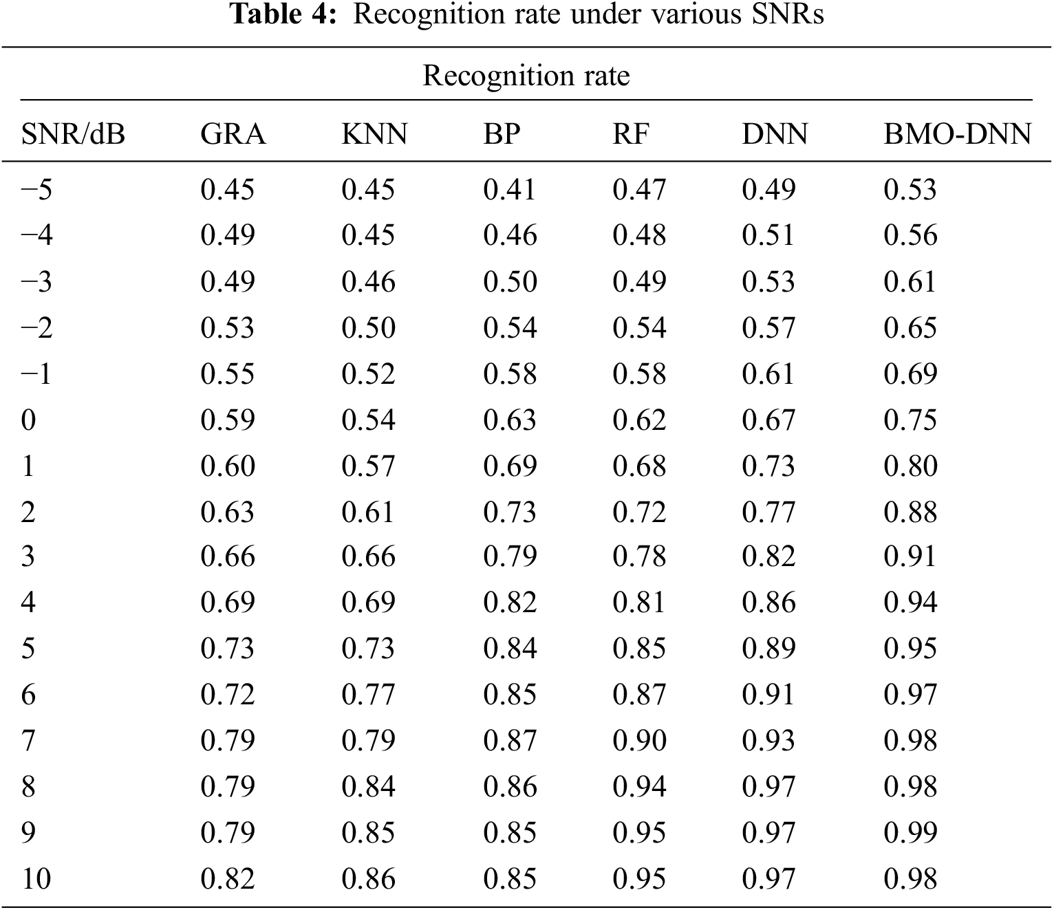
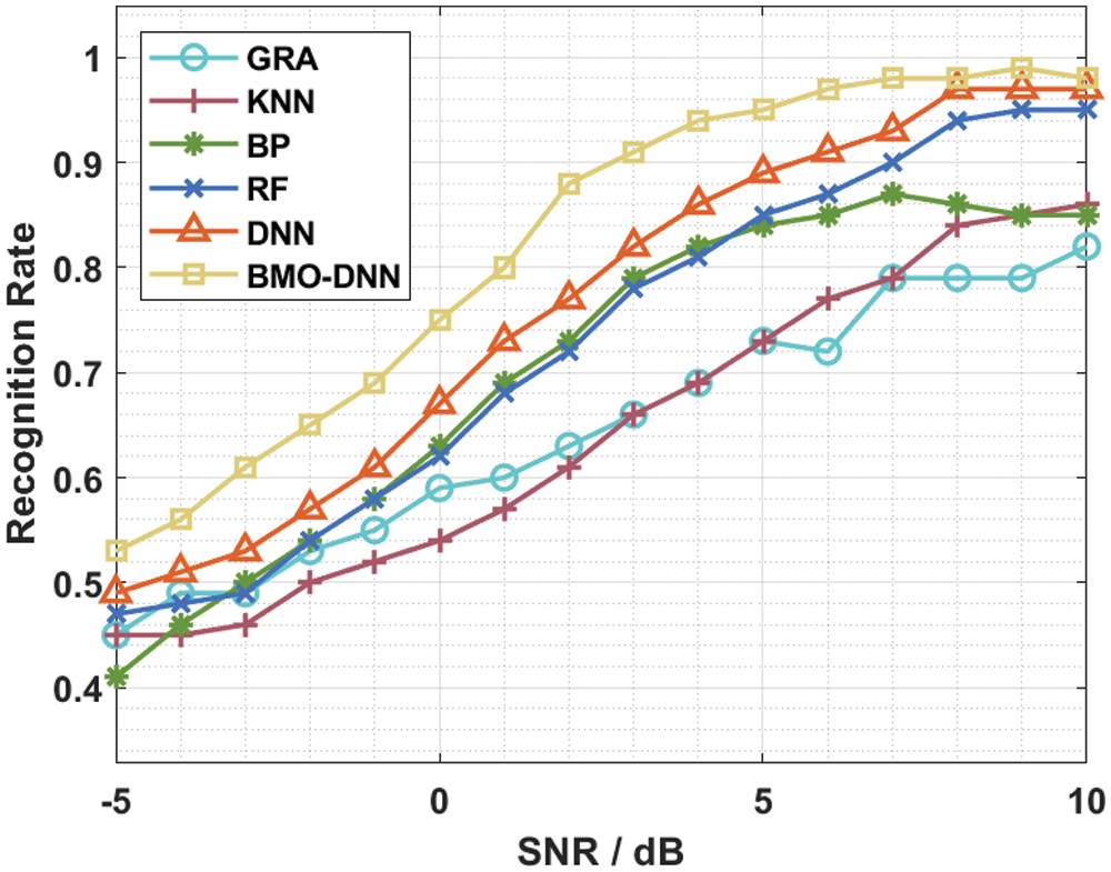
Figure 7: Recognition rate under various SNRs

In order to guarantee the improved modulation signal recognition rate of the BMO-DNN technique, a brief comparison study is made under varying SNR in Tab. 4 and Fig. 7. The results demonstrated that the BMO-DNN technique has accomplished maximum recognition rate under varying SNRs. For instance, with −5dB, the BMO-DNN technique has obtained a higher recognition rate of 0.53 whereas the GRA, KNN, BP, RF, and DNN techniques have achieved a lower recognition rate of 0.45, 0.45, 0.41, 0.47, and 0.49.

Moreover, with −1dB, the BMO-DNN approach has attained a maximum recognition rate of 0.69 whereas the GRA, KNN, BP, RF, and DNN algorithms have reached a lesser recognition rate of 0.55, 0.52, 0.58, 0.58, and 0.61. Eventually, with 2dB, the BMO-DNN algorithm has obtained an increased recognition rate of 0.88 whereas the GRA, KNN, BP, RF, and DNN techniques have achieved a lower recognition rate of 0.63, 0.61, 0.73, 0.72, and 0.77. Meanwhile, with 5dB, the BMO-DNN method has obtained an enhanced recognition rate of 0.95 whereas the GRA, KNN, BP, RF, and DNN approaches have gained a minimal recognition rate of 0.73, 0.73, 0.84, 0.85, and 0.89. At the same time, with 8dB, the BMO-DNN technique has obtained a superior recognition rate of 0.98 whereas the GRA, KNN, BP, RF, and DNN algorithms have gained a lesser recognition rate of 0.79, 0.84, 0.86, 0.94, and 0.97. At last, with 10dB, the BMO-DNN approach has obtained a higher recognition rate of 0.98 whereas the GRA, KNN, BP, RF, and DNN methodologies have reached a minimum recognition rate of 0.82, 0.86, 0.85, 0.95, and 0.97. The experimental outcomes pointed out the superior recognition rate of the CSM-FFDNN model over the recent state of art methods interms of different evaluation parameters due to the DNN based classification, and BMO based hyperparameter optimization.

5  Conclusion

In this study, a new CSM-FFDNN model is designed to classify various kinds of digitally modulated signals such as ASK, FSK, BPSK, and QAM. The proposed CSM-FFDNN model involves three major processes namely fractal FE, DNN based classification, and BMO based hyperparameter optimization. Besides, the extracted features are fed into the DNN model for modulation signal classification. To improve the classification performance of the DNN model, a BMO is used for the hyperparameter tuning of the DNN model in such a way that the DNN performance can be raised. A comprehensive experimental analysis is made to point out the improved outcomes of the CSM-FFDNN model. The experimental outcomes pointed out the superior recognition rate of the CSM-FFDNN model over the recent state of art methods interms of different evaluation parameters. In future, advanced DL models can be used to classify the digitally modulated signals.

Funding Statement: This work was supported by the National Research Foundation of Korea (NRF) grant funded by the Korea government (MSIT) (No. 2021R1F1A1063319).

Conflicts of Interest: The authors declare that they have no conflicts of interest to report regarding the present study.

References

 1.  A. Abdelmutalab, K. Assaleh and M. El-Tarhuni, “Automatic modulation classification based on high order cumulants and hierarchical polynomial classifiers,” Physical Communication, vol. 21, no. 8, pp. 10–18, 2016. [Google Scholar]

 2.  K. Shankar, A. R. W. Sait, D. Gupta, S. K. Lakshmanaprabu, A. Khanna et al., “Automated detection and classification of fundus diabetic retinopathy images using synergic deep learning model,” Pattern Recognition Letters, vol. 133, no. Dec (3), pp. 210–216, 2020. [Google Scholar]

 3.  O. A. Dobre, A. Abdi, Y. B. Ness and W. Su, “Survey of automatic modulation classification techniques: Classical approaches and new trends,” IET Communications, vol. 1, no. 2, pp. 137, 2007. [Google Scholar]

 4.  I. V. Pustokhina, D. A. Pustokhin, T. Vaiyapuri, D. Gupta, S. Kumar et al., “An automated deep learning based anomaly detection in pedestrian walkways for vulnerable road users safety,” Safety Science, vol. 142, no. 11, pp. 105356, 2021. [Google Scholar]

 5.  C. Weber, M. Peter and T. Felhauer, “Automatic modulation classification technique for radio monitoring,” Electronics Letters, vol. 51, no. 10, pp. 794–796, 2015. [Google Scholar]

 6.  T. Vaiyapuri, S. N. Mohanty, M. Sivaram, I. V. Pustokhina, D. A. Pustokhin et al., “Automatic vehicle license plate recognition using optimal deep learning model,” Computers, Materials & Continua, vol. 67, no. 2, pp. 1881–1897, 2021. [Google Scholar]

 7.  H. Li and M. Li, “Analysis of the pattern recognition algorithm of broadband satellite modulation signal under deformable convolutional neural networks,” PLOS ONE, vol. 15, no. 7, pp. e0234068, 2020. [Google Scholar]

 8.  J. Uthayakumar, N. Metawa, K. Shankar and S. K. Lakshmanaprabu, “Intelligent hybrid model for financial crisis prediction using machine learning techniques,” Information Systems and e-Business Management, vol. 18, no. 4, pp. 617–645, 2020. [Google Scholar]

 9.  S. Zhang, L. Yao, A. Sun and Y. Tay, “Deep learning based recommender system: A survey and new perspectives,” ACM Computing Surveys, vol. 52, no. 1, pp. 1–38, 2019. [Google Scholar]

10. R. J. S. Raj, S. J. Shobana, I. V. Pustokhina, D. A. Pustokhin, D. Gupta et al., “Optimal feature selection-based medical image classification using deep learning model in internet of medical things,” IEEE Access, vol. 8, pp. 58006–58017, 2020. [Google Scholar]

11. C. T. Shi, “Signal pattern recognition based on fractal features and machine learning,” Applied Sciences, vol. 8, no. 8, pp. 1327, 2018. [Google Scholar]

12. A. Ali, F. Yangyu and S. Liu, “Automatic modulation classification of digital modulation signals with stacked autoencoders,” Digital Signal Processing, vol. 71, pp. 108–116, 2017. [Google Scholar]

13. S. Zhou, Z. Yin, Z. Wu, Y. Chen, N. Zhao et al., “A robust modulation classification method using convolutional neural networks,” EURASIP Journal on Advances in Signal Processing, vol. 2019, no. 1, pp. 55, 2019. [Google Scholar]

14. X. Zhang, J. Sun and X. Zhang, “Automatic modulation classification based on novel feature extraction algorithms,” IEEE Access, vol. 8, pp. 16362–16371, 2020. [Google Scholar]

15. Y. Wang, J. Yang, M. Liu and G. Gui, “LightAMC: Lightweight automatic modulation classification via deep learning and compressive sensing,” IEEE Transactions on Vehicular Technology, vol. 69, no. 3, pp. 3491–3495, 2020. [Google Scholar]

16. D. Hong, Z. Zhang and X. Xu, “Automatic modulation classification using recurrent neural networks,” in 2017 3rd IEEE Int. Conf. on Computer and Communications (ICCC), Chengdu, China, pp. 695–700, 2017. [Google Scholar]

17. Y. Wang, J. Wang, W. Zhang, J. Yang and G. Gui, “Deep learning-based cooperative automatic modulation classification method for MIMO systems,” IEEE Transactions on Vehicular Technology, vol. 69, no. 4, pp. 4575–4579, 2020. [Google Scholar]

18. Y. S. Liang, “Fractal dimension of riemann-liouville fractional integral of 1-dimensional continuous functions,” Fractional Calculus and Applied Analysis, vol. 21, no. 6, pp. 1651–1658, 2018. [Google Scholar]

19. S. Ramesh and D. Vydeki, “Recognition and classification of paddy leaf diseases using optimized deep neural network with jaya algorithm,” Information Processing in Agriculture, vol. 7, no. 2, pp. 249–260, 2020. [Google Scholar]

20. S. Ahmed, K. K. Ghosh, S. K. Bera, F. Schwenker and R. Sarkar, “Gray level image contrast enhancement using barnacles mating optimizer,” IEEE Access, vol. 8, pp. 169196–169214, 2020. [Google Scholar]

This work is licensed under a Creative Commons Attribution 4.0 International License, which permits unrestricted use, distribution, and reproduction in any medium, provided the original work is properly cited.