DOI:10.32604/csse.2022.027288
| Computer Systems Science & Engineering DOI:10.32604/csse.2022.027288 | |
| Article |
Spatio-Temporal Wind Speed Prediction Based on Variational Mode Decomposition
1School of Computer and Science, Nanjing University of Information Science and Technology, Nanjing, 210044, China
2Department of Electrical and Computer Engineering, University of Windsor, Windsor, N9B 3P4, Canada
*Corresponding Author: Yingnan Zhao. Email: zh_yingnan@126.com
Received: 13 January 2022; Accepted: 21 March 2022
Abstract: Improving short-term wind speed prediction accuracy and stability remains a challenge for wind forecasting researchers. This paper proposes a new variational mode decomposition (VMD)-attention-based spatio-temporal network (VASTN) method that takes advantage of both temporal and spatial correlations of wind speed. First, VASTN is a hybrid wind speed prediction model that combines VMD, squeeze-and-excitation network (SENet), and attention mechanism (AM)-based bidirectional long short-term memory (BiLSTM). VASTN initially employs VMD to decompose the wind speed matrix into a series of intrinsic mode functions (IMF). Then, to extract the spatial features at the bottom of the model, each IMF employs an improved convolutional neural network algorithm based on channel AM, also known as SENet. Second, it combines BiLSTM and AM at the top layer to extract aggregated spatial features and capture temporal dependencies. Finally, VASTN accumulates the predictions of each IMF to obtain the predicted wind speed. This method employs VMD to reduce the randomness and instability of the original data before employing AM to improve prediction accuracy through mapping weight and parameter learning. Experimental results on real-world data demonstrate VASTN’s superiority over previous related algorithms.
Keywords: Short-term wind speed prediction; variational mode decomposition; attention mechanism; SENet; BiLSTM
Wind energy, as one of the most environmentally friendly renewable resources, has obvious benefits, such as cleanliness, low cost, and sustainability. It has become the primary renewable energy source and is rapidly developing globally [1]. Wind power’s intermittent nature, randomness, and instability, however, pose challenges to wind power generation systems [2].
Accurate wind speed prediction is critical for wind energy conversion system configuration, scheduling, maintenance, and planning [3]. Four main conventional wind speed algorithms are currently in use: 1) physical methods, 2) statistical methods, 3) spatial correlation methods, and 4) artificial intelligence (AI) methods. A physical method, such as numerical weather prediction, is to develop a physical or meteorological information model, such as temperature, air pressure, humidity, topography, and air density, to predict wind speed over time [4]. However, this method necessitates complex calculations and performs poorly in short-term wind speed forecasts [5]. Based on big historical data, statistical methods use mathematical equations to predict wind speed [6]. Autoregressive moving average model, moving average model, autoregressive model (AR), and autoregressive integrated moving average model are some of its representative methods [7]. For prediction, spatial correlation methods rely on the interaction of wind speed at different wind speed observation sites [8]. AI methods are not dependent on a precise model of the object. Instead, they learn the relationships between inputs and outputs using historical data. Consequently, they are appropriate for random nonlinear systems. Deep learning algorithms, such as multilayer perception (MLP) [9], recurrent neural network (RNN) [10], convolutional neural network (CNN) [11], gated recurrent unit (GRU), long short-term memory (LSTM), and others have been used for short-term wind speed prediction since the development of deep learning.
Traditional AI methods are simple to implement and can be adapted in various ways. However, due to the randomness and intermittent nature of wind speed, traditional AI methods still have room for improvement. In this regard, the academic community has proposed a hybrid prediction model based on modal decomposition methods to obtain relatively stable wind velocity subsequences, such as empirical mode decomposition (EMD), which is good at processing nonlinear nonstationary signals [12], ensemble empirical mode decomposition (EEMD), which is an improved method for EMD mixing phenomenon [13], and complete ensemble empirical mode decomposition, which is based on EEMD, eliminating the unclean noise removal of EEMD [14]. The VMD method is robust to sampling and noise and overcomes the limitations of EMD to a certain extent. Comparative studies show that the VMD hybrid model outperforms a single prediction model in terms of prediction accuracy [15–17], so this study employs VMD to decompose wind speed series.
Currently, most researchers focus on selecting input variables in the prediction process while ignoring the different impact levels of various model features on the output. Furthermore, most AI wind speed prediction methods only extract temporal features. In recent years, research interest in capturing spatial features has increased. Consequently, this paper proposes a new method for predicting wind speed based on CNN’s attention mechanism (AM) and the BiLSTM deep learning network based on VMD decomposition. First, the wind farm’s spatio-temporal wind speed is used as input data to build SENet, a CNN architecture that uses the AM to weigh channel features. It can pay more attention to the effectiveness and reduce the impact of useless features while extracting spatial features. The data containing spatial features are then transferred to the BiLSTM-Attention layer, which extracts temporal features. To strengthen the influence of important information, different weights are assigned to the hidden state of BiLSTM using mapping weights and parameter learning. This method addresses the issue of the existing wind speed prediction AI models’ insufficient accuracy.
The remainder of the paper is organized as follows: Section 2 explains the basic principles of the algorithm’s framework; Section 3 illustrates a detailed introduction to the VASTN network architecture; Section 4 discusses the experimental results and compares them with other typical algorithms; Section 5 summarizes the entire paper.
2.1 Variational Mode Decomposition
VMD is a new signal decomposition technology proposed by Dragomiretskiy et al. [18] that is primarily used to decompose an input signal into a discrete number of subsignals known as modes. First, VMD decomposes the original signal into a bandwidth with a center pulsation based on the number of modes specified. The alternate direction multiplier method (ADMM) is then used to update each mode and its corresponding center pulsation, gradually demodulating each mode to its corresponding baseband. Finally, it extracts each mode and the associated center pulsation.
Assuming that the data to be processed is f, each mode is uk and its center frequency is ωk. The specific process of VMD is as follows.
1) To obtain the unilateral spectrum, compute the analytic signal associated with each mode using Hilbert transform.
2) The frequency spectrum of each mode is modulated to the baseband by exponentially mixing the analytical signal of each mode and the corresponding center frequency.
3) To obtain the gradient square L-norm, the signal is demodulated using Gaussian smoothness. It has the following variational constraint model.
4) Use the quadratic penalty function α and the Lagrange multiplier λ to find the optimal solution to the abovementioned variational constrained model. The constrained variational problem is transformed into a nonconstrained variational problem, and the resulting Lagrangian function is as follows.
5) Finally, the ADMM method is used to solve the unconstrained variational problem, and uk and ωk are updated continuously throughout the solution process. Finally, each uk can complete the frequency band division based on the frequency domain characteristics of f and realize the adaptive signal decomposition. The following are the new uk and ωk of the solution.
uk and ωk do not stop updating until they meet the following criteria.
ɛ is a given level of accuracy greater than 0.
Hu et al. proposed squeeze-and-excitation networks (SENet), a CNN-based AM that learns the features of different channels. SENet refers to the “squeeze-and-excitation” (SE) block of learning the relationship between the CNN convolution kernel’s channels. It employs the channel AM to adaptively recalibrate channel-wise feature responses by explicitly modeling the interdependencies. Finally, the SENet architecture combines the SE block with the general CNN network [19].
CNN is a feedforward neural network with a deep structure that employs convolutional calculations [20]. As a representative deep learning model, it uses trainable convolution kernels, local pooling operations, and fully connected operations to alternately apply the results of forward and backpropagations to the raw input to extract spatial features [21]. Due to its superior performance, CNN has been widely used to extract spatial features in various fields, including machine vision [22], voice recognition [23], and text processing.
The structure of an SE block is depicted in Fig. 1. First, following the traditional convolution operation, the size of the convolution kernel is compressed to 1 × 1 × C using the global average pool. The weight of each channel is then calculated through the excitation operation and assigned to the convolution kernel. Where Ftr represents a convolution operation with the following input and output:
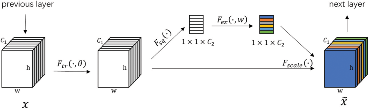
Figure 1: A typical squeeze-and-excitation block
The formula of Ftr is as follows.
where uc represents the c-th two-dimensional (2D) matrix in the three-dimensional (3D) matrix U and
SENet proposes a squeeze step to address the problem of not utilizing channel correlation. To focus on the channel information, the spatial features are compressed using global average pooling. Eq. (8) transforms the input of W × H × C into the output of 1 × 1 × C.
The purpose of the excitation operation is to fully capture the channel dependencies. Therefore, it employs a straightforward gating mechanism with sigmoid activation.
In Eq. (9), z is the squeeze output, W1, W2 are fully connected layer operation, δ indicates a ReLU layer operation. And then the output go through the sigmoid function σ to get s which is to characterize the weights of c feature maps in matrix U. This weight is learned by training the previous fully connected and nonlinear layers end-to-end.
Finally, the SE block applies the calculated channel weight to each matrix using Eq. (10), where sc is the weight of c-th matrix U.
LSTM is proposed as the main component of BiLSTM to overcome limitations such as gradient vanishing and long-term dependence of recurrent neural networks (RNN). Furthermore, because of its superiority in dealing with sequential data, LSTM has found widespread application in video analysis [24], speech recognition [25], signal analysis [26], etc.
LSTM introduces a gate mechanism to control the circulation and loss of features to solve the long-term dependence problem of RNN. Fig. 2 depicts the transmission of data characteristics between several adjacent LSTM cells, where Xt, ht, and ct represent the input data, output value, and unit state at time t, respectively.
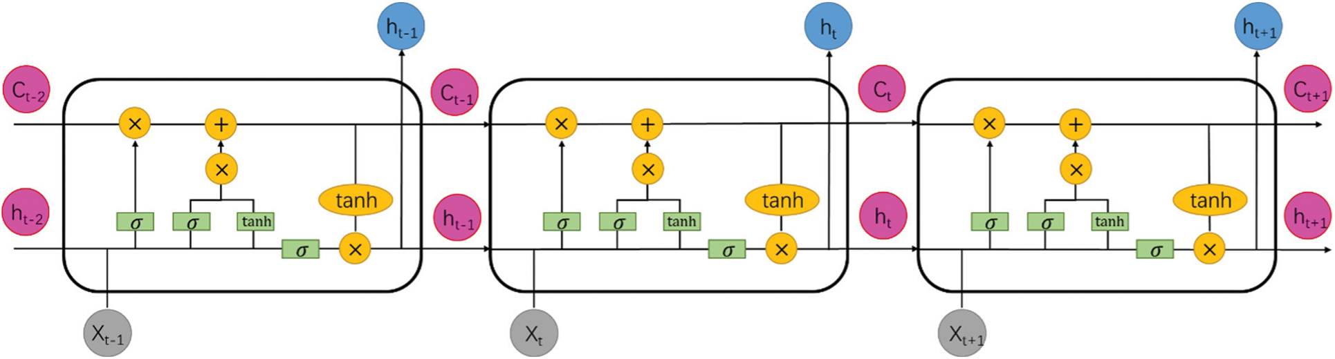
Figure 2: Structure of long short-term memory (LSTM) units
Each LSTM unit employs three gates to determine whether the information is retained or lost, as shown by the six formulas below, where w represents the input matrix, b denotes a bias vector, and σ is an activation function:
1). The forget gate: The forget gate ft determines how much of the unit state ct−1 at the previous moment is retained in the current moment ct.
2). The input gate: The input gate it determines the amount of network input xt saved to the unit state ct at the current time.
3). The output gate: The output gate ot controls the proportion of the current output value ht output by the control unit status ct to the LSTM.
4). Unit status update value
5). Unit state ct.
6). Output value ht.
BiLSTM is an extension of regular LSTM, which comprises forward and backward LSTMs (i.e., left-to-right and right-to-left). First, it employs LSTM on the forward input sequence. The reverse input sequence is then fed into the LSTM model. Consequently, the model’s accuracy can be improved because using the LSTM twice can greatly improve the long-term dependence [27]. Recent research has shown that this method can also predict wind speed [28].
A difficult problem is retaining the spatio-temporal correlation of data without increasing the amount of data. Dimension reduction is an efficient preprocessing method of spatio-temporal wind speed data, which can remove noise and unimportant features of high-dimensional data and subsequently improve data processing speed [29]. In this paper, the spatial wind speed matrix proposed [30] is a practical solution for organizing spatio-temporal wind speed data into two dimensions (SWSM). Typically, our dataset comes from a 2D array, which can be represented by an M × N grid and each wind speed station by coordinates (i, j)(1 ≤ i ≤ M, 1 ≤ j ≤ N) (Fig. 3a). The wind speed in the time dimension is a one-dimensional time series for each wind speed station (Fig. 3b). Consequently, multiple continuous-time SWSM can represent the 3D distribution of all wind speeds in time and space.
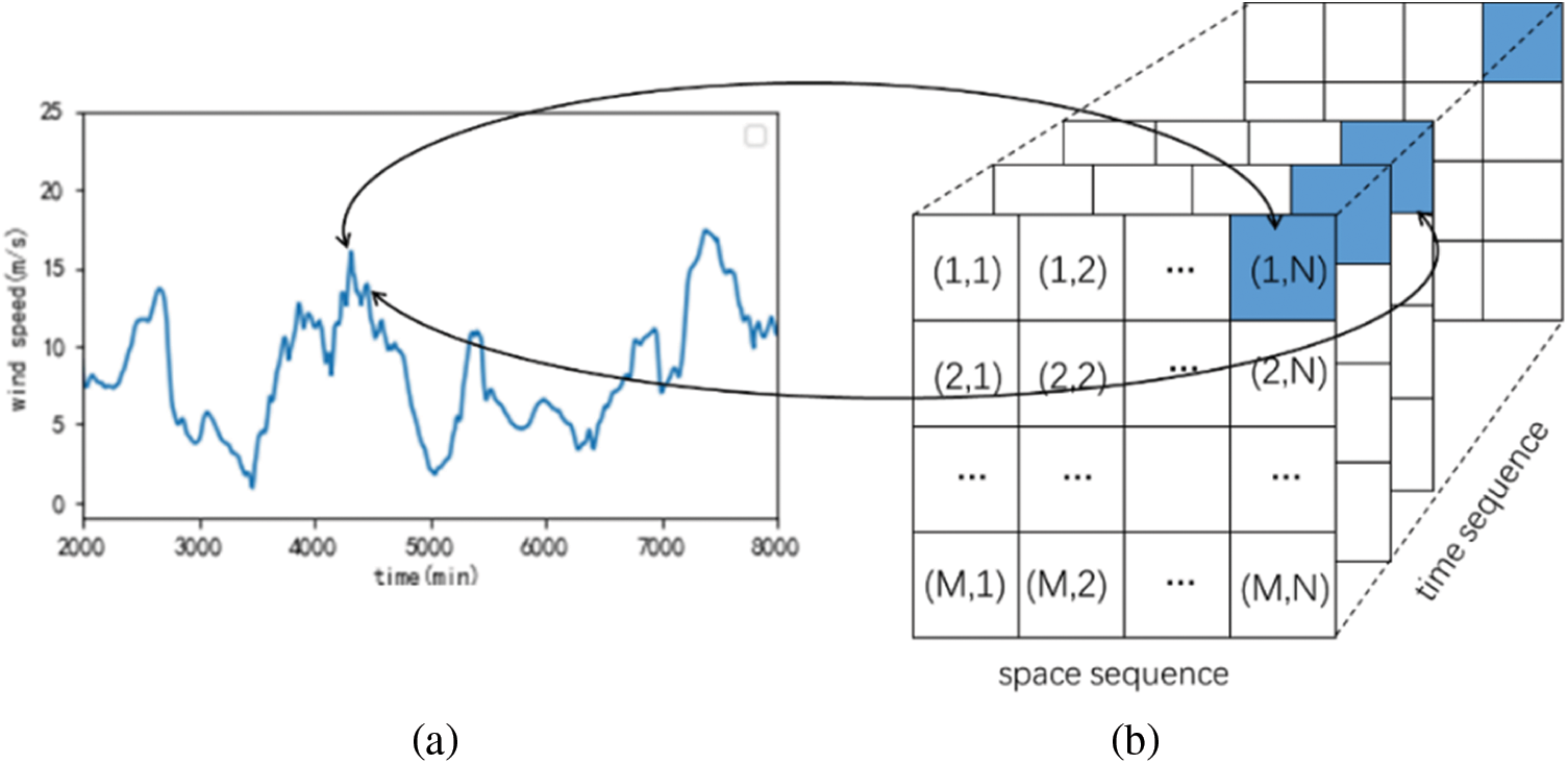
Figure 3: (a) A wind speed time series. (b) A series of spatio-temporal wind speed data into two dimensions (SWSM)
Another issue is that VMD is typically used to decompose time series, making it difficult to act directly on 3D spatio-temporal data. In this case, we improved SWSM to solve it (Fig. 4), where k is the number of modes.
1) After completing the SWSM, extract and save the wind speed for each time series separately.
2) Using VMD, decompose each time series separately and obtain IMF1, IMF2, … IMFk for each time sequence.
3) The IMFs are divided into k sub-SWSMs based on their positions.
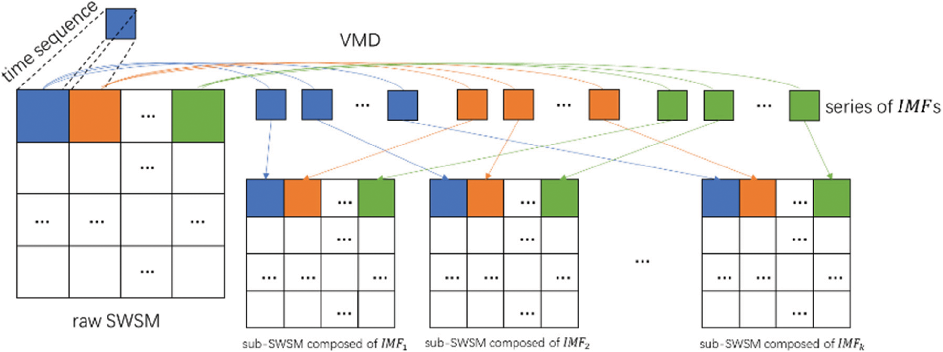
Figure 4: Steps to generate sub-SWSM composed of intrinsic mode functions (IMFs)
3.2 The Basic Strategy for VASTN
Removing irrelevant data from the deep hybrid architecture can significantly reduce unnecessary training time and prevent overfitting. Consequently, the VASTN algorithm first removes all useless data from the selected original data, leaving only the wind speed, corresponding time, and geographic location information to ensure the dataset’s temporal and spatial correlation. The original SWSM with solid nonlinearity and randomness is then decomposed using VMD into a series of sub-SWSM composed of IMF. Next, we use the SENet-BiLSTM-Attention hybrid framework for model training and prediction for each sub-SWSM component and obtain the predicted value of each IMF. Finally, the predicted values of each IMF are superimposed to obtain the final predicted wind speed. Fig. 5 depicts the flow chart for the preceding procedure.
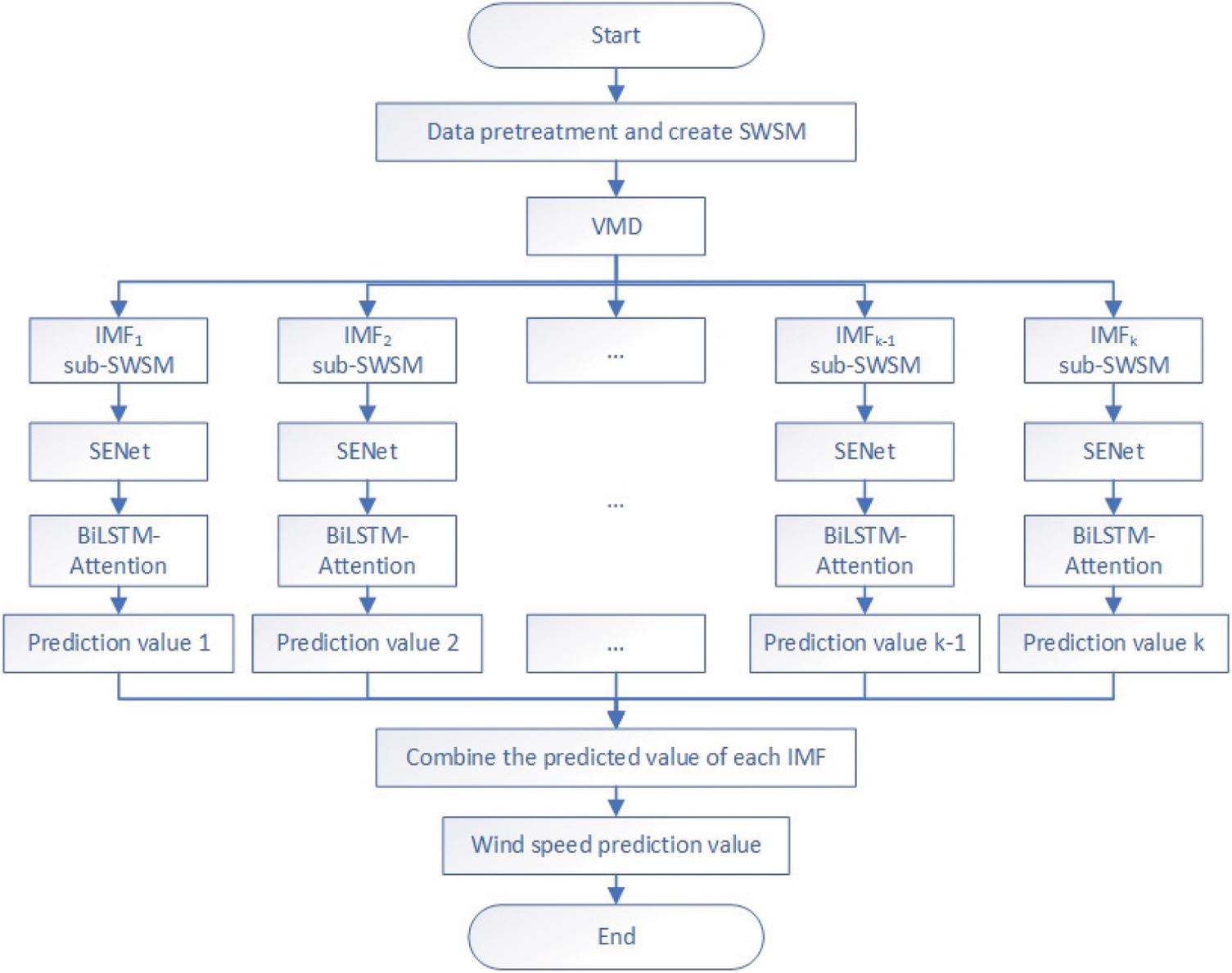
Figure 5: The flowchart of variational mode decomposition-attention-based spatio-temporal network (VASTN)
Following the data processing described above and the use of VMD, we must extract the features of the sub-SWSM, i.e., the extraction of spatial features and the capture of temporal features.
The spatial features are extracted using SENet. It has the following advantages: 1) The topology-preserving nature of kernels enables CNNs to fully and directly utilize spatial attributes from a single SWSM [31]. 2) SENet can learn to use global information to selectively emphasize channels’ information and suppress useless information without increasing computational complexity [19].
Herein, we use a combination of BiLSTM and an AM as the time model to capture the extracted spatial features in time sequences, with the following advantages: 1) LSTM can analyze the dependencies within the sequence by capturing both long-term and short-term time characteristics to meet different forecasting needs. 2) Because BiLSTM traverses time series in both directions, it is more effective than general LSTM at extracting time features [32]. 3) Finally, by combining the AM and BiLSTM, the model can focus on more important features, reducing training time complexity while increasing prediction accuracy.
Fig. 6a depicts the overall network framework proposed by the paper, At the model’s base, CNN is used to extract the spatial characteristics of a single wind speed matrix that can be viewed as a grayscale image. The SE block then accepts the output of the CNN layer to emphasizes critical channel information while weakening useless information, analyzing spatial correlation in the wind farm. Next, we use a fully connected layer to change the dimensionality of the SENet output so that it can be input into the BiLSTM layer. In the model’s upper layer, we use BiLSTM to capture temporal features among previously extracted spatial features bidirectionally. The AM can simultaneously improve efficiency and accuracy. Finally, the top layer can output the current IMF forecast value, which is combined with other IMF forecast results to produce the final wind speed forecast value.
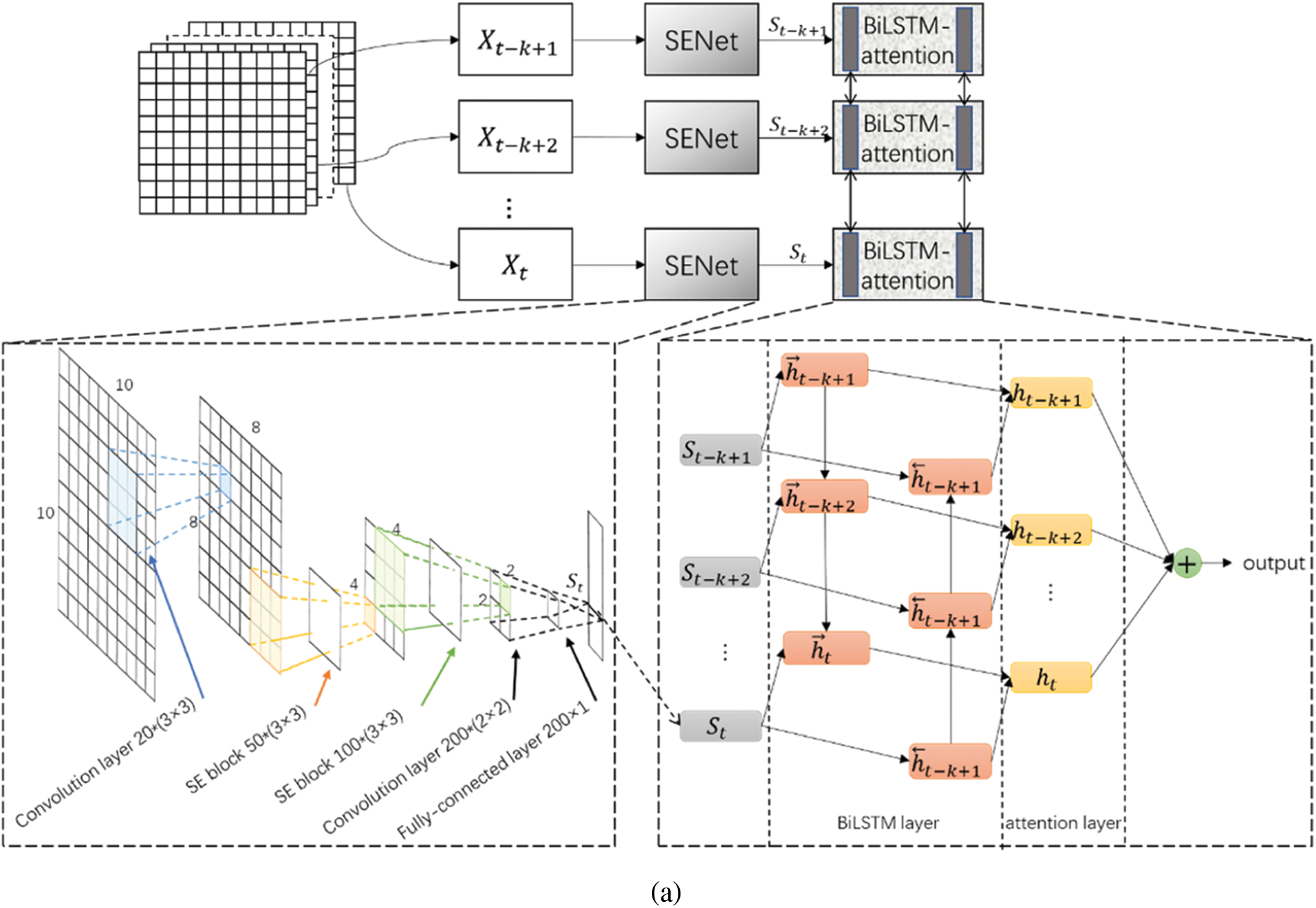
Figure 6: (a) The process of the network framework
The mixed model can be jointly trained using a loss function defined as a mean squared error (MSE).
where n is the total data count, yi represents the i-th actual wind speed, and
The training error propagates down the model backward during model training, i.e., the backpropagation (BP) algorithm, widely used in various domains such as surgical simulation [33]. The error difference propagates from the BiLSTM-Attention layer to the SENet layer and the underlying CNN. Consequently, each layer can adjust parameters using the training error. Another potential advantage is that the spatial model (SENet) can adapt based on temporal data. Similarly, the temporal model (BiLSTM-Attention) can adjust based on spatial data [30]. This way, space and time learning can be coupled together, allowing the entire framework to learn spatio-temporal features simultaneously.
The National Renewable Energy Laboratory provides the Wind Integration National Dataset Toolkit, which is a dataset that realistically reflects the ramping characteristics, spatial and temporal correlations, and capacity factors of simulated wind plants. It includes wind speed data with a 5-min resolution for over 126,000 land-based and offshore wind power production sites across the continental United States from 2007 to 2013 [34].
This paper uses 100 wind speed datasets with 52560 frames at ten-minute intervals generated from a 10 × 10 wind turbine matrix in New Mexico at 36.5 latitude and −103.3 longitude for the whole year of 2012, with the highest wind speed being 32.77 m/s and the lowest wind speed being 0.02 m/s.
The parameters of the VMD algorithm are as follows: the number of modes K, the penalty term α, the fidelity coefficient τ, and the convergence tolerance level ɛ. Studies have shown that τ and ɛ can usually take default values [35]; hence, the difficulty and focus of the VMD algorithm lies in determining how to select the appropriate K and α. Herein, the values of K and α refer to the method [36], and we conduct multiple experiments to determine K = 8, α = 2000, and τ = 0.3. In terms of the frequency spectrum of the decomposition mode, a very small K can result in signal under-segmentation, while too many modes can result in pattern repetition or additional noise [36]. Fig. 7a depicts the decomposition result, and Fig. 7b depicts the absence of modal aliasing in the decomposition result, indicating that the decomposition achieves a relatively ideal effect.
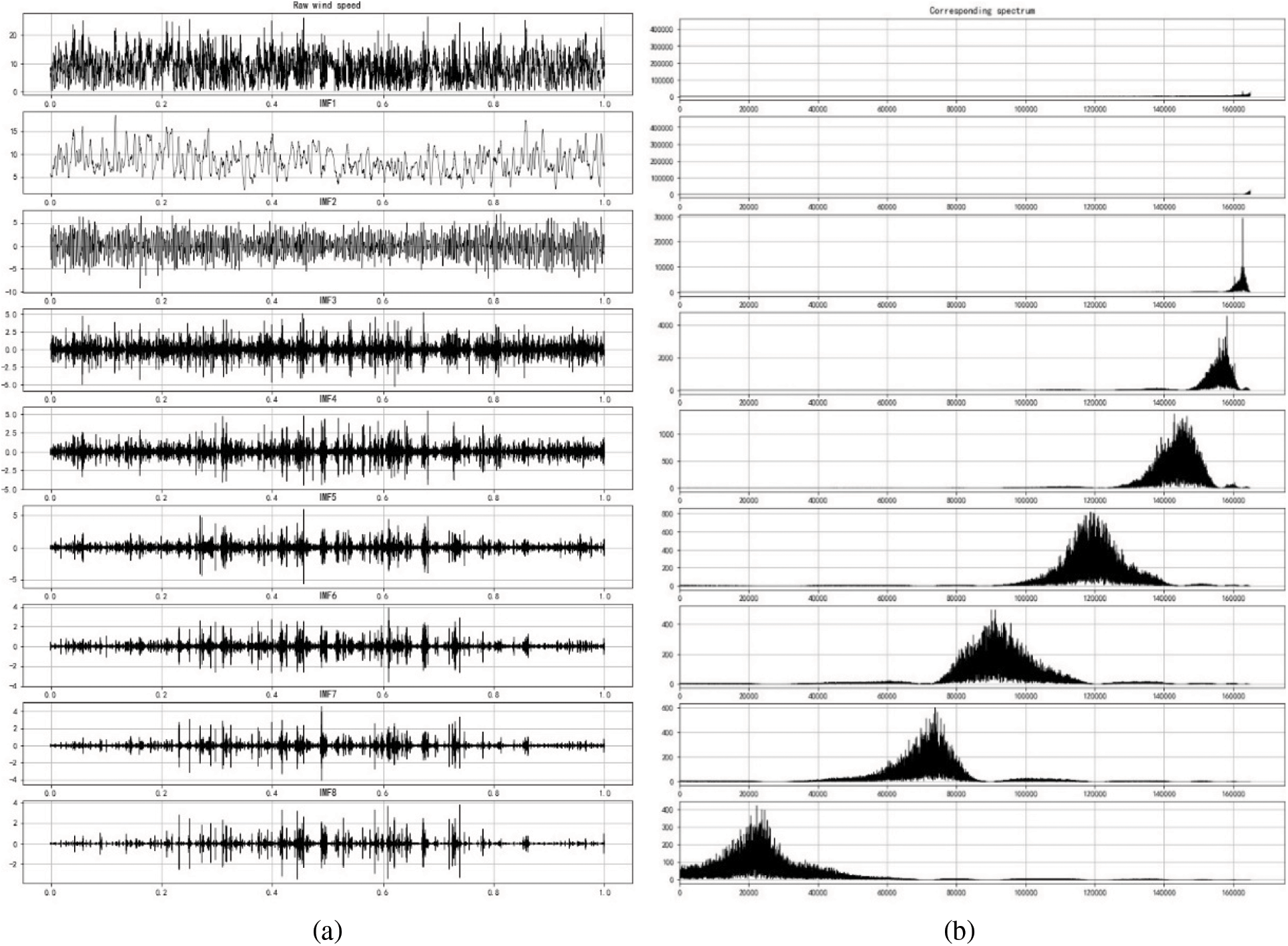
Figure 7: (a) Variational mode decomposition (VMD) diagram of a time series (b) Spectrogram of each IMF
This paper compares the prediction results of the VASTN model and other algorithms using the root mean square error (RMSE), mean absolute error (MAE), mean absolute percent error (MAPE), and Pearson correlation (COR). The evaluation criteria are as follows.
where n denotes the number of predicted data, yi represents the i-th actual wind speed,
To implement the network, the experiment employs the Keras2.4.2 framework with the TensorFlow2.4 backend. A CPU E5-2689 16-core 16G, GPU NVIDIA GeForce RTX 3070, 8G video memory, and 200 GB solid-state drive comprise the experimental server environment.
In a prediction task, the dataset is divided into three parts: the first 60% of the frames are the training set, the next 10% are the validation set, and the remaining 30% are the test set. The training set is one of them, and its purpose is to train the model. The validation set is used to monitor the model’s quality, save the best model in real-time during training, and use the test set to evaluate the model’s predicted performance. Simultaneously, we use early stopping in the validation set to improve the model performance and prevent overfitting. As previously stated, the training set, validation set, and test set in this article contain 31536, 5256, and 15768 frames, respectively. There may be a few differences in the frame number in each set depending on the prediction horizon. Also, in order to show the superiority of VASTN in short-term wind speed forecasting, and to find out the best time point for VASTN forecasting, we set the prediction horizon of 10, 20, 30, 60, 120 min in the experiment.
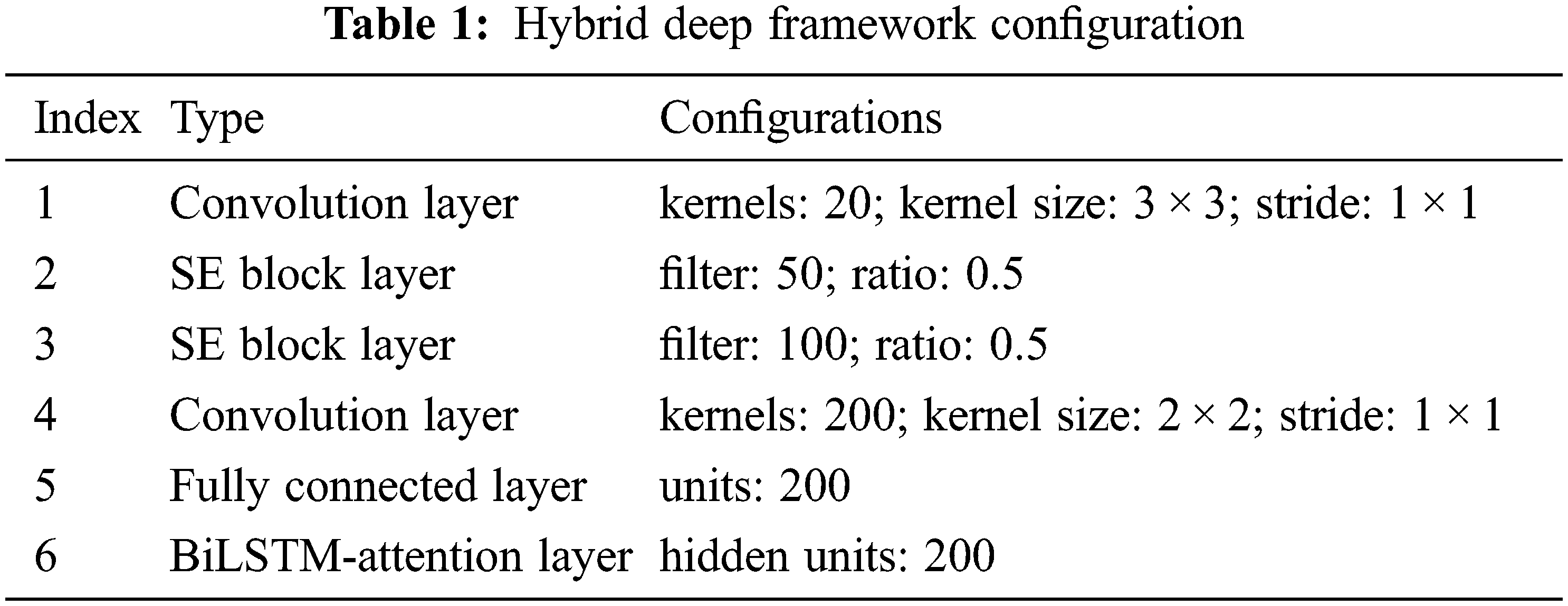
VASTN is trained using the Adagrad optimization algorithm, with the training epoch set to 100. Tab. 1 shows that the deep hybrid framework’s optimization algorithm and hyperparameters are derived from experiments.
To validate the proposed VASTN’s superior performance, we compare it with the following wind speed prediction AI models: LSTM, multilayer perceptron (MLP), recurrent neural network (RNN), and predictive spatio-temporal network (PSTN) [30]. Simultaneously, to validate the effectiveness of each component of the hybrid framework, we set up some VASTN submodels for comparison, namely the SENet-BiLSTM-Attention, BiLSTM-Attention, and VMD-CNN-LSTM model.
LSTM, MLP, RNN are AI algorithms that can capture temporal dependencies in a temporally dynamic manner, but they cannot capture features of spatial data.
PSTN is a spatio-temporal wind speed prediction model instead of other typical algorithms. Its model framework is divided into two parts: CNN and LSTM. CNN extracts the spatial features of the data, while LSTM captures the temporal features and finally obtains the predicted value.
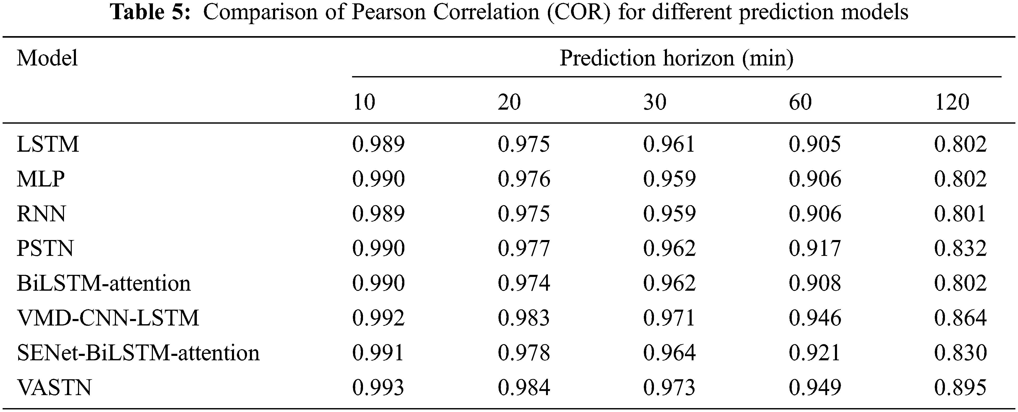
Tabs. 2 to 5 show a comparison of the RMSE, MAE, MAPE, and COR of the various prediction models. VASTN has clearly demonstrated superiority across all prediction horizons and evaluation criteria. When the prediction horizon is 10, 20, 30, 60, and 120 min, the RMSE of VASTN is 13%, 20%, 16%, 21%, and 19% lower than that of PSTN, with an average reduction of 17%. The average optimization of MAE and MAPE is 18% and 28%, respectively, indicating that VASTN has significant advantages over the traditional wind speed prediction model.
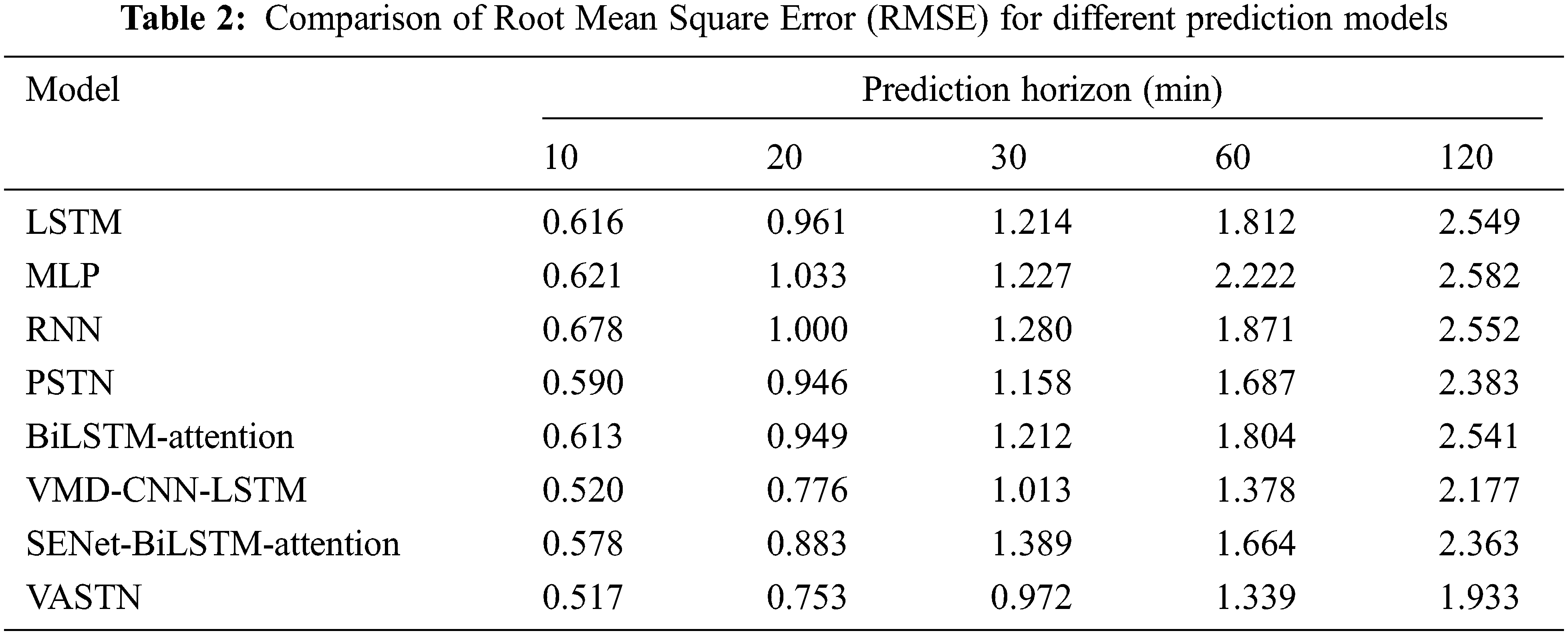
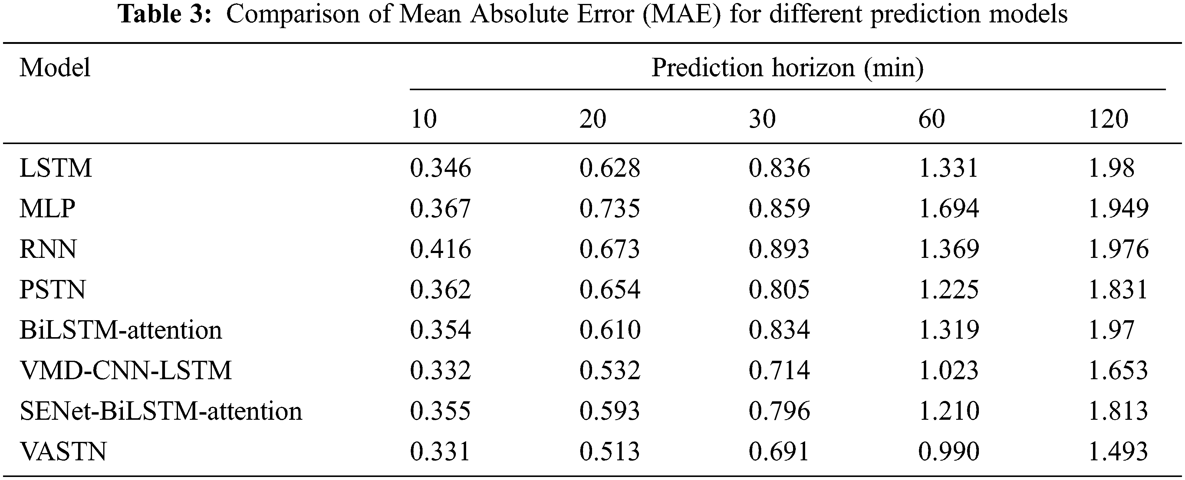
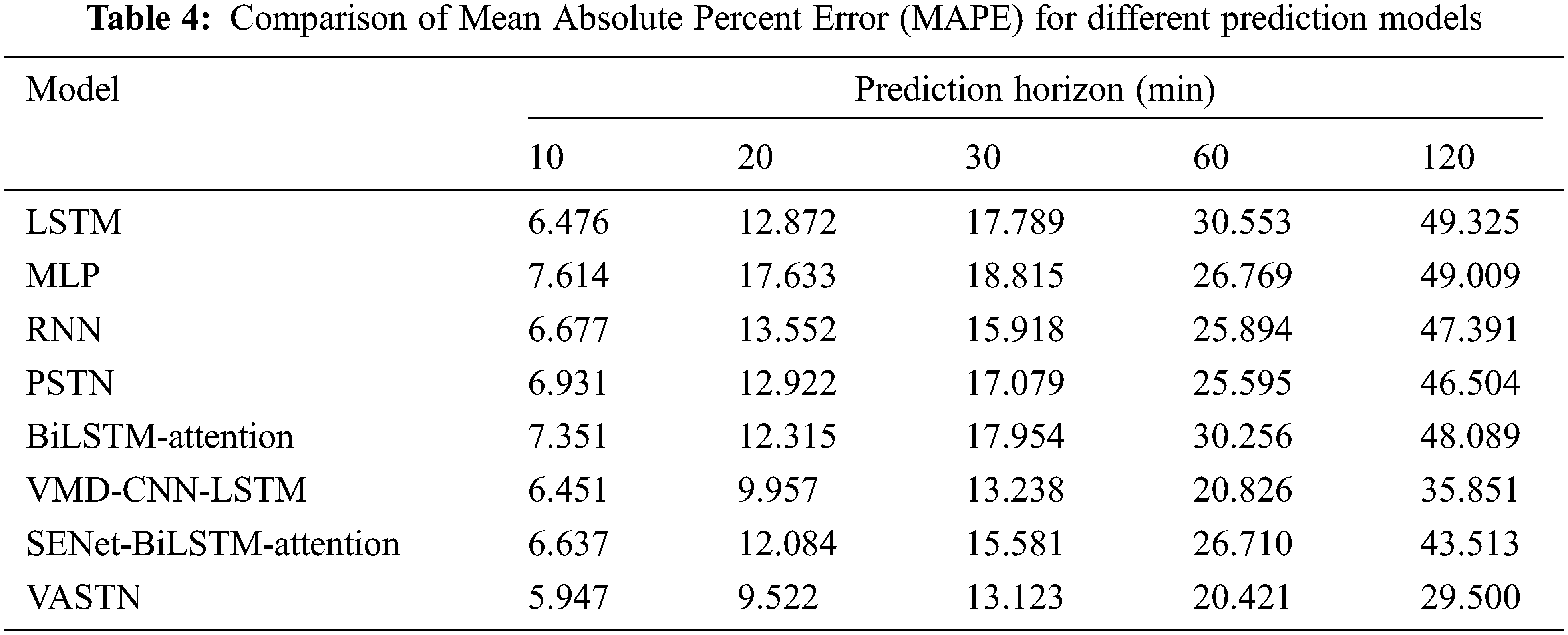
Furthermore, for the SENet-BiLSTM-Attention submodel that does not use VMD decomposition, VASTN reduces the RMSE, MAE, and MAPE by an average of 20%, 16%, and 25%, respectively. Similarly, the VMD-CNN-LSTM submodel outperforms PSTN by 14%, 13%, and 21%, respectively. It demonstrates that VMD decomposition can better eliminate wind speed randomness and unevenness for short-term wind speed forecasting, resulting in better forecast results. Furthermore, compared to general LSTM, BiLSTM has specific optimizations in RMSE, MAE, and MAPE. Similarly, VASTN has a 6%, 6%, and 10% improvement in these three aspects compared to the VMD-CNN-LSTM submodel of the algorithm that does not use the AM, demonstrating the model’s optimization after the introduction of the AM. Compared with the spatio-temporal model PSTN, the best-performing model in the time sequence model, BiLSTM-Attention, improves RMSE, MAE, and MAPE by 5%, 4%, and 6%, respectively. It shows that the model’s temporal and spatial characteristics are generally superior to the time sequence model, indicating that spatio-temporal data contains more features conducive to wind speed prediction than pure time series data.
Fig. 8 depicts the prediction results of the VASTN model proposed in the paper for the 20-min prediction horizon. The predicted value of the VASTN model is consistent with the actual value. When there is no apparent fluctuation in wind speed, the residual analysis results show that the model’s prediction residuals can be uniformly and randomly distributed on both sides of the zero baselines. Conversely, only when the wind speed changes dramatically can it deviate further. This suggests that systematic errors are rare in the modeling process. Fig. 9 compares 20-min wind speed prediction results of different typical models and VASTN, including VASTN, LSTM, MLP, RNN, and PSTN. Fig. 10 compares the prediction results of VASTN and its submodels, including SENet-BiLSTM-Attention, BiLSTM-Attention, and VMD-CNN-LSTM. Figs. 9 and 10 demonstrate the VASTN algorithm’s superiority in short-term wind speed prediction.
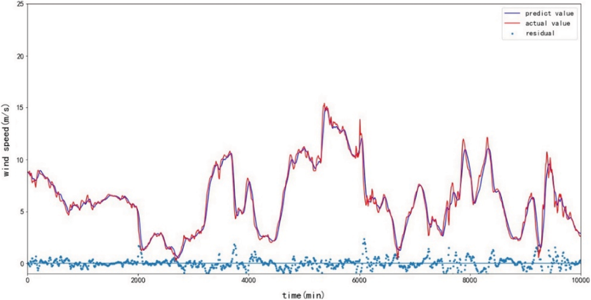
Figure 8: 20-min VASTN prediction results and residual chart
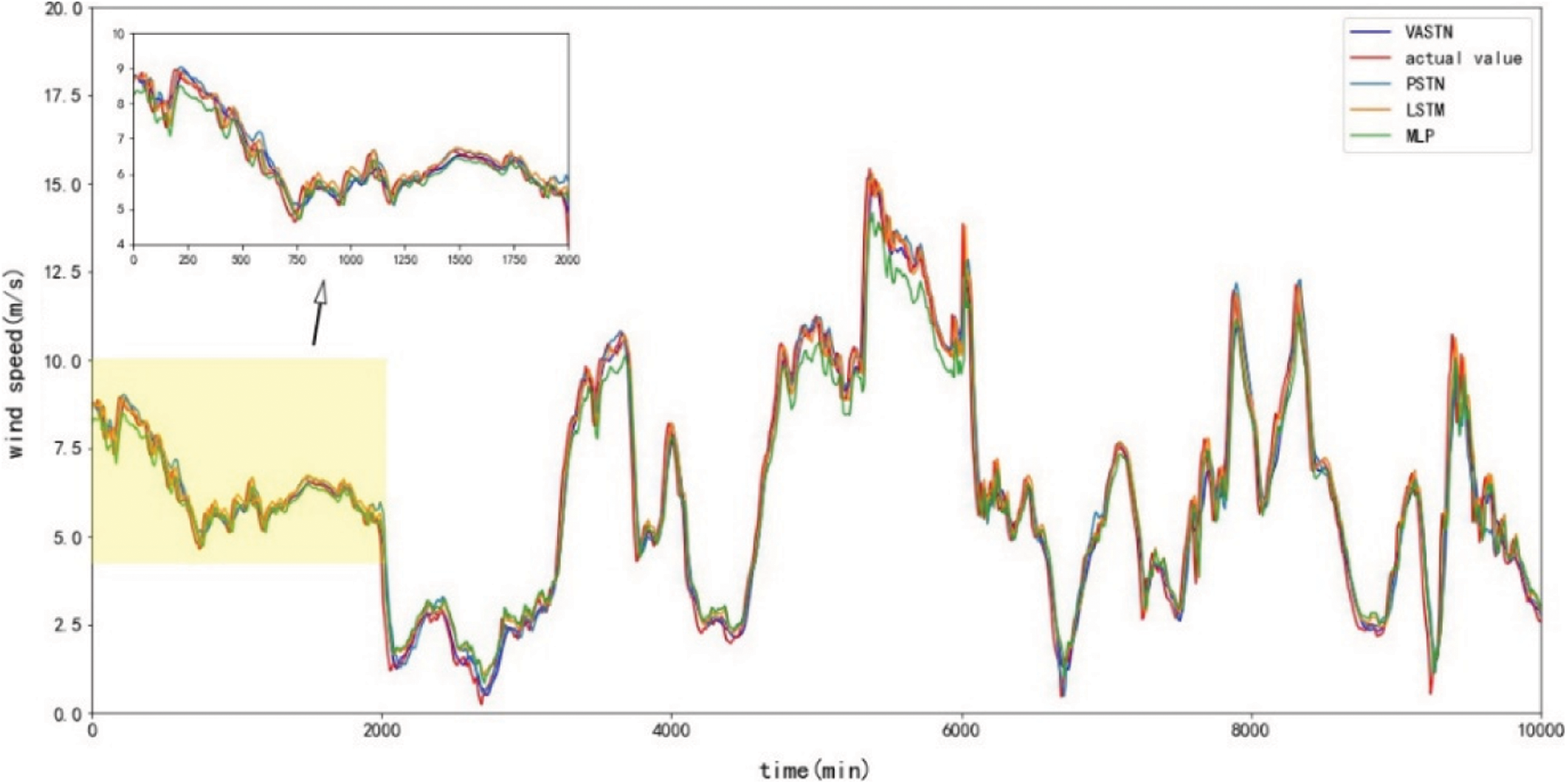
Figure 9: 20-min typical model comparison chart
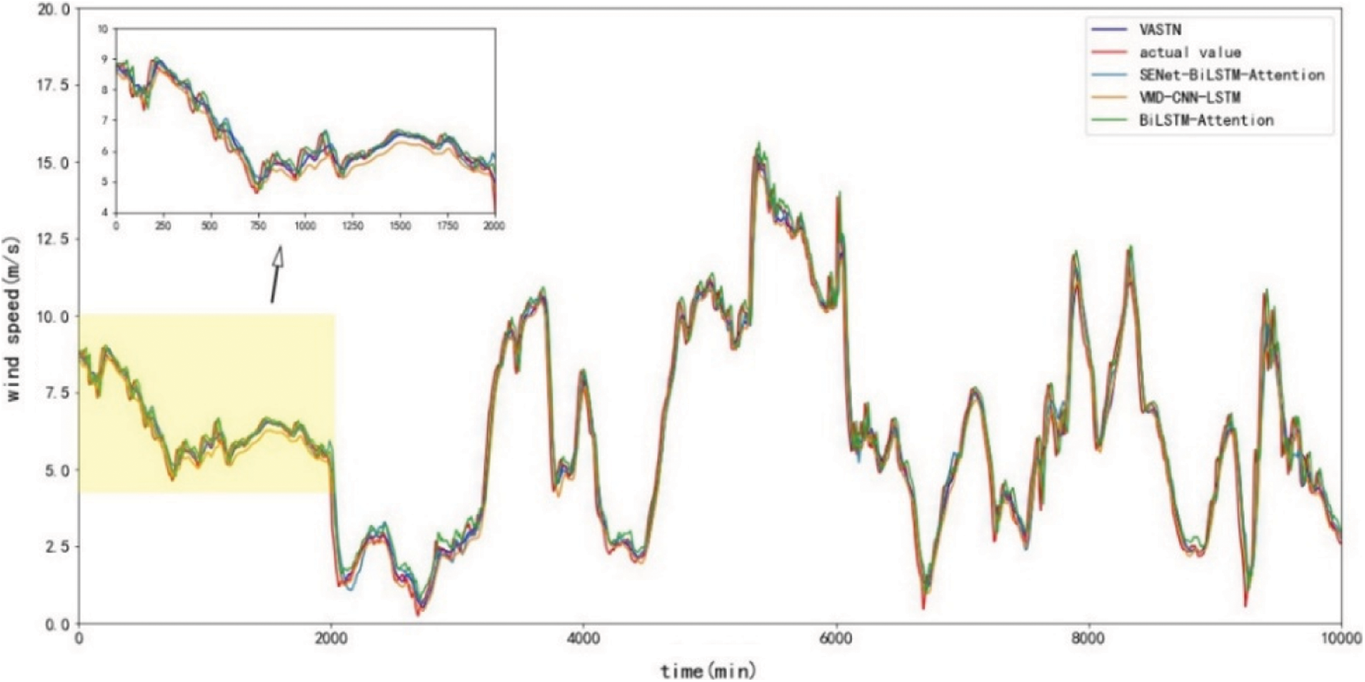
Figure 10: 20-min submodel comparison chart
Accurately and efficiently predict short-term wind speed is still a challenging problem. To solve this problem, this paper proposes VASTN, a new hybrid deep framework for short-term wind speed prediction, which integrates the learning of wind speed’s temporal and spatial characteristics into a unified framework. First, VMD decomposition reduces the randomness of wind speed. The spatial properties of the wind speed matrix are then extracted using SENet, and the time properties are weighted and extracted using BiLSTM-Attention. Finally, the proposed model combines the results of each IMF’s prediction to obtain the wind speed prediction value. Experiments on real-world datasets show that the VASTN algorithm outperforms the traditional short-term wind speed prediction algorithm. It also demonstrates the accuracy of VMD, the AM, and the extraction of temporal and spatial wind speed features in short-term wind speed prediction.
In future work, we will use the improved VMD algorithm to automatically adjust and select the optimal VMD parameters. In addition, we will attempt to improve the algorithm’s accuracy and efficiency by employing other AM methods, such as spatial attention or channel and spatial hybrid attention.
Acknowledgement: This paper is supported by the undergraduate training program for innovation and entrepreneurship of NUIST (XJDC202110300239).
Funding Statement: The authors received no specific funding for this study.
Conflicts of Interest: The authors declare that they have no conflicts of interest to report regarding the present study.
1. R. K. Grace and R. Manimegalai, “Design of neural network based wind speed prediction model using two,” Computer Systems Science and Engineering, vol. 40, no. 2, pp. 593–606, 2022. [Google Scholar]
2. S. Fan, J. R. Liao, R. Yokoyama, L. Chen and W. J. Lee, “Forecasting the wind generation using a two-stage network based on meteorological information,” IEEE Transactions on Energy Conversion, vol. 24, no. 2, pp. 474–482, 2009. [Google Scholar]
3. Q. H. Hu, R. J. Zhang and Y. C. Zhou, “Transfer learning for short-term wind speed prediction with deep neural networks,” Renewable Energy, vol. 85, pp. 83–95, 2016. [Google Scholar]
4. L. Landberg, “Short-term prediction of the power production from wind farms,” Journal of Wind Engineering and Industrial Aerodynamics, vol. 80, no. 1–2, pp. 207–220, 1999. [Google Scholar]
5. G. Giebel, R. Brownsword, G. N. Kariniotakis, M. D. Denhard and C. Draxl, “The state-of-the-art in short-term prediction of wind power. A literature overview,” Denmark, 2011. [Online]. Available: http://www.risoe.dtu.dk/rispubl/NEI/NEI-DK-5521.pdf. [Google Scholar]
6. H. Liu, H. Q. Tian and Y. F. Li, “Comparison of two new arima-ann and arima-kalman hybrid methods for wind speed prediction,” Applied Energy, vol. 98, pp. 415–424, 2012. [Google Scholar]
7. G. Y. Wu, Y. Xiao and S. S. Weng, “Discussion about short-term forecast of wind speed on wind farm,” Jilin Electric Power, vol. 181, no. 5, pp. 21–24, 2005. [Google Scholar]
8. T. G. Barbounis and J. B. Theocharis, “A locally recurrent fuzzy neural network with application to the wind speed prediction using spatial correlation,” Information Sciences, vol. 177, no. 24, pp. 5775–5797, 2007. [Google Scholar]
9. H. Liu, H. Q. Tian and Y. F. Li, “Comparison of new hybrid feemd-mlp, feemd-anfis, wavelet packet-mlp and wavelet packet-anfis for wind speed predictions,” Energy Conversion and Management, vol. 89, pp. 1–11, 2015. [Google Scholar]
10. T. G. Barbounis, J. B. Theocharis, M. Alexiadis and P. Dokopoulos, “Long-term wind speed and power forecasting using local recurrent neural network models,” IEEE Transactions on Energy Conversion, vol. 21, no. 1, pp. 273–284, 2006. [Google Scholar]
11. L. Bai, E. Crisostomi, M. Raugi and M. Tucci, “Wind power forecast using wind forecasts at different altitudes in convolutional neural networks,” in 2019 IEEE Power & Energy Society General Meeting (PESGM), IEEE, Atlanta, Georgia, USA, pp. 1–5, 2020. [Google Scholar]
12. H. Ashraf, A. Waris, S. O. Gilani, M. U. Tariq and H. Alquhayz, “Threshold parameters selection for empirical mode decomposition-based emg signal denoising,” Intelligent Automation & Soft Computing, vol. 27, no. 3, pp. 799–815, 2021. [Google Scholar]
13. S. X. Wang, N. Zhang, L. Wu and Y. M. Wang, “Wind speed forecasting based on the hybrid ensemble empirical mode decomposition and ga-bp neural network method,” Renewable Energy, vol. 94, pp. 629–636, 2016. [Google Scholar]
14. M. E. Torres, M. A. Colominas, G. Schlotthauer and P. Flandrin, “A complete ensemble empirical mode decomposition with adaptive noise,” in IEEE international conference on acoustics, speech and signal processing (ICASSP), IEEE, Prague, Czech Republic, pp. 4144–4147, 2011. [Google Scholar]
15. T. L. Fu, “A hybrid prediction of wind speed based on variational mode decomposition method and long short-term memory,” in 2020 Int. Conf. on Computer Engineering and Application (ICCEA), IEEE, Guangzhou, China, pp. 408–412, 2020. [Google Scholar]
16. J. M. Gonzalez-Sopena, V. Pakrashi and B. Ghosh, “Multi-step ahead wind power forecasting for Ireland using an ensemble of VMD-ELM models,” in 2020 31st Irish Signals and Systems Conf. (ISSC), IEEE, Letterkenny, Ireland, pp. 1–5, 2020. [Google Scholar]
17. Z. X. Sun and M. Zhao, “Short-term wind power forecasting based on VMD decomposition, ConvLSTM networks and error analysis,” IEEE Access, vol. 8, pp. 134422–134434, 2020. [Google Scholar]
18. K. Dragomiretskiy and D. Zosso, “Variational mode decomposition,” IEEE Transactions on Signal Processing, vol. 63, no. 3, pp. 531–544, 2014. [Google Scholar]
19. J. Hu, L. Shen and G. Sun, “Squeeze-and-excitation networks,” in Proc. of the IEEE Conf. on Computer Vision and Pattern Recognition, Salt Lake Cit, State of Utah, USA, pp. 7132–7141, 2018. [Google Scholar]
20. X. Zhu, R. Liu, Y. Chen, X. Gao, Y. Wang et al., “Wind speed behaviors feather analysis and its utilization on wind speed prediction using 3D-CNN,” Energy, vol. 236, pp. 121523, 2021. [Google Scholar]
21. S. Ji, W. Xu, M. Yang and K. Yu, “3D convolutional neural networks for human action recognition,” IEEE Transactions on Pattern Analysis & Machine Intelligence, vol. 35, no. 1, pp. 221–231, 2012. [Google Scholar]
22. A. G. Howard, M. L. Zhu, B. Chen, D. Kalenichenko, W. J. Wang et al., “Mobilenets: Efficient convolutional neural networks for mobile vision applications,” arXiv preprint arXiv:1704.04861, 2017. [Google Scholar]
23. R. V. Sharan, S. Berkovsky and S. Liu, “Voice command recognition using biologically inspired time-frequency representation and convolutional neural networks,” in 2020 42nd Annual Int. Conf. of the IEEE Engineering in Medicine and Biology Society (EMBC) in Conjunction with the 43rd Annual Conf. of the Canadian Medical and Biological Engineering Society, IEEE, Montreal, QC, Canada, pp. 998–1001, 2020. [Google Scholar]
24. J. Amin, M. A. Anjum, M. Sharif, S. Kadry, Y. Nam et al., “Convolutional bi-lstm based human gait recognition using video sequences,” Computers, Materials & Continua, vol. 68, no. 2, pp. 2693–2709, 2021. [Google Scholar]
25. Z. Wang, T. Zhang, Y. Shao and B. Ding, “LSTM-Convolutional-BLSTM encoder-decoder network for minimum mean-square error approach to speech enhancement,” Applied Acoustics, vol. 172, pp. 107647, 2021. [Google Scholar]
26. L. Liao, J. Liu, X. Wu, F. Zhou, J. Pan et al., “Time difference penalized traffic signal timing by LSTM Q-network to balance safety and capacity at intersections,” IEEE Access, vol. 8, pp. 80086–80096, 2020. [Google Scholar]
27. P. Baldi, S. Brunak, P. Frasconi, G. Soda and G. Pollastri, “Exploiting the past and the future in protein secondary structure prediction,” Bioinformatics, vol. 15, no. 11, pp. 937–946, 1999. [Google Scholar]
28. S. Siami-Namini, N. Tavakoli and A. S. Namin, “The performance of LSTM and BiLSTM in forecasting time series,” in 2019 IEEE Int. Conf. on Big Data (Big Data), IEEE, Los Angeles, CA, USA, pp. 3285–3292, 2019. [Google Scholar]
29. X. R. Zhang, W. F. Zhang, W. Sun, X. M. Sun and S. K. Jha, “A robust 3-d medical watermarking based on wavelet transform for data protection,” Computer Systems Science and Engineering, vol. 41, no. 3, pp. 1043–1056, 2022. [Google Scholar]
30. Q. Zhu, J. Chen, D. Shi, L. Zhu, X. Bai et al., “Learning temporal and spatial correlations jointly: A unified framework for wind speed prediction,” IEEE Transactions on Sustainable Energy, vol. 11, no. 1, pp. 509–523, 2019. [Google Scholar]
31. R. Y. Li, W. Sheng, F. Y. Zhu and J. Huang, “Adaptive graph convolutional neural networks,” Proc. of the AAAI Conf. on Artificial Intelligence, vol. 32, no. 1, 2018. [Online]. Available: https://ojs.aaai.org/index.php/AAAI/article/view/11691. [Google Scholar]
32. S. Siami-Namini, N. Tavakoli and A. S. Namin, “A comparative analysis of forecasting financial time series using ARIMA, LSTM, and BiLSTM,” arXiv preprint arXiv:1911.09512, 2019. [Google Scholar]
33. X. Zhang, X. Sun, W. Sun, T. Xu, P. Wang et al., “Deformation expression of soft tissue based on bp neural network,” Intelligent Automation & Soft Computing, vol. 32, no. 2, pp. 1041–1053, 2022. [Google Scholar]
34. C. Draxl, A. Clifton, B. M. Hodge and J. McCaa, “The wind integration national dataset (WIND) toolkit,” Applied Energy, vol. 151, pp. 355–366, 2015. [Google Scholar]
35. D. W. Yang, F. Z. Feng, Y. D. Hao, P. C. Jiang and C. Ding, “A VMD sample entropy feature extraction method and its application in planetary gearbox fault diagnosis,” Journal of Vibration and Shock, vol. 37, no. 16, pp. 198–205, 2018. [Google Scholar]
36. J. Fang, “Research on fault diagnosis of marine gearbox based on variational mode decomposition,” M.S. dissertation, Wuhan University of Technology, China, 2017. [Google Scholar]
 | This work is licensed under a Creative Commons Attribution 4.0 International License, which permits unrestricted use, distribution, and reproduction in any medium, provided the original work is properly cited. |