DOI:10.32604/csse.2022.023680
| Computer Systems Science & Engineering DOI:10.32604/csse.2022.023680 | |
| Article |
Classification of Glaucoma in Retinal Images Using EfficientnetB4 Deep Learning Model
National Engineering College, Kovilpatti, 628502, India
*Corresponding Author: N. B. Prakash. Email: nbprakas@gmail.com
Received: 16 September 2021; Accepted: 29 November 2021
Abstract: Today, many eye diseases jeopardize our everyday lives, such as Diabetic Retinopathy (DR), Age-related Macular Degeneration (AMD), and Glaucoma. Glaucoma is an incurable and unavoidable eye disease that damages the vision of optic nerves and quality of life. Classification of Glaucoma has been an active field of research for the past ten years. Several approaches for Glaucoma classification are established, beginning with conventional segmentation methods and feature-extraction to deep-learning techniques such as Convolution Neural Networks (CNN). In contrast, CNN classifies the input images directly using tuned parameters of convolution and pooling layers by extracting features. But, the volume of training datasets determines the performance of the CNN; the model trained with small datasets, overfit issues arise. CNN has therefore developed with transfer learning. The primary aim of this study is to explore the potential of EfficientNet with transfer learning for the classification of Glaucoma. The performance of the current work compares with other models, namely VGG16, InceptionV3, and Xception using public datasets such as RIM-ONEV2 & V3, ORIGA, DRISHTI-GS1, HRF, and ACRIMA. The dataset has split into training, validation, and testing with the ratio of 70:15:15. The assessment of the test dataset shows that the pre-trained EfficientNetB4 has achieved the highest performance value compared to other models listed above. The proposed method achieved 99.38% accuracy and also better results for other metrics, such as sensitivity, specificity, precision, F1_score, Kappa score, and Area Under Curve (AUC) compared to other models.
Keywords: Convolution neural network; deep learning; fundus image; glaucoma; image classification
Visual impairment currently represents human society’s most challenging challenges. Approximately 285 million individuals worldwide are impaired by vision, and 39 million suffer from complete and irreversible blindness, says the World Health Organization (WHO) [1,2]. Glaucoma is the second leading cause of global vision loss. “In 2013, around 64 million cases reported worldwide, estimates of 80 million and 111.8 million cases by 2020 and 2040 respectively affecting a crucial portion of the World’s population” [3,4]. Glaucoma is an irrevocable neuro-degenerative eye disease. There is no symptom in the beginning and gradually damages the optic nerve by causing permanent vision loss. The optic nerve damage causes the structural change of the optic nerve head called Optic Disc (OD). The OD region has divided into two: an Optic Cup (OC), the brightest region of the disc, and a peripheral area called the neuro-retinal rim, where the nerve fibers bend to the cup zone [5] as shown in Fig. 1a. The OC has gradually increased with the disease progress, and the neuro-retinal rim diluted in the disc region. Due to this structure of OD region changes and its shown in Fig. 1b.
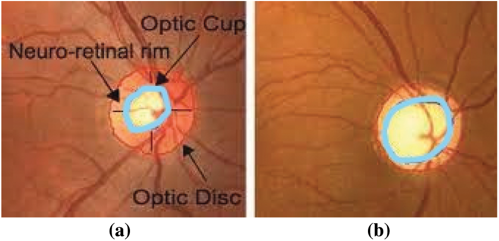
Figure 1: Fundus image of (a) healthy optic disc (b) glaucoma affected eye
The expert can assess the structural changes in the OD region, which is a traditional way to evaluate Glaucoma. However, this assessment is unique; the testing duration is considerable, expensive, and uncomfortable for the patients. Another technique of assessing disease, utilizing retinal imaging studies, is a more promising and successful approach for Glaucoma screening [6]. Many research activities have been carried out employing retinal images and have obtained good diagnostic accuracy. This evaluation method decreases the expert’s burden and is helpful for bulk screening.
The location of the optic nerve head and retinal nerve fiber layer is the first step in automatic glaucoma detection [7], followed by segmentation of the OC and OD areas to measure parameters like the Cup-to-Disk Ratio (CDR) [8], ISNT (Inferior Superior Nasal Temporal) [9], RNFL (Retinal Nerve Fiber Layer) thickness [10], and peripapillary atrophy [11] using 2D fundus images. However, when dealing with a wide range of clinical circumstances, this can be not easy. With the detection of Glaucoma, the worst identification of OD or erroneous segmentation of OC and OD is an ongoing worry [12]. As a result, overcoming the limitations of existing methods in glaucoma screening is momentous.
The classification of disease must be more accurate, so we decided to carry on further research to achieve higher accuracy than existing methods in the classification task without extracting features of the input image. So we have chosen Deep CNN as a means to achieve our aim. Recently, Deep CNN has become dominant in automated medical image analysis, and many researchers have reported that it can outperform well. CNN can automatically extract the image features by tuning the parameters of the convolution and the pooling layers.
Wong et al. [8] proposed level-set techniques to evaluate the CDR after obtaining the OD and OC masks. They found that the measured CDR value shows a variation of units of 0.2 compared to the ground truth when tested on 104 images. Joshi et al. [13] proposed a method to segment OC using vessel bends in the cup boundary and the circular Hough transform to obtain CDR. Yin et al. [14] have suggested a method that combines edge detection and Hough transformation with a statistical model for the automatic OD segmentation that has extended to a cup broader on the blood vessel removed OD image. This method is evaluated on 325 test images and obtains an average dice coefficient of 0.92 for OD segmentation and 0.81 for OC segmentation, respectively. Cheng et al. [12] proposed a superpixel technique for OD and OC segmentation, with overlapping errors of 9.5% and 24.1%, respectively. An automatic glaucoma diagnosis using stochastic watershed transformation to segment the OC was proposed by Diaz-Pinto et al. [15] and obtained specificity of 0.81 and sensitivity of 0.87, respectively.
The drawback of the above methods for glaucoma detection, measurement of CDR, Area Cup/Disc ratio (ACDR), and vascular kinks position. These can show an error in evaluation from that of ground truth marked by more than one expert. Automatic feature extraction has been focused on by convolutional neural networks (CNNs), and Bock et al. [16] suggested a data-driven method that leverages image Eigen to extract features and categorized them using a support vector machine (SVM). This method was evaluated by a private dataset with 575 images and obtained an AUC of 0.88. However, this method cannot be compared with our study because they use a private dataset.
In 1898, introduced the first CNN’s biological-inspired variants of multilayer perceptron. The performance of CNN’s has improved with GPUs, rectifiers, new regularization, and augmentation techniques for automatic annotation using ImageNet datasets [17,18]. At various levels of abstraction, the CNN architectures can extract highly distinctive features. The first layer of CNN is the input layer, used to extract the images feature at specific directions and locations. The middle layer of the CNN identifies the edges like structures. In the last few layers, matching familiar objects have been detected from the more complex structures. The computational resources and a large number of labeled data were necessary to train the CNN from scratch for glaucoma assessment. For that, the larger dataset, such as ImageNet, has been used by the CNN model to train.
For medical images applications, Carneiro et al. [19] suggested that CNN models trained on ImageNet improve the model’s performance. According to Chen et al. [20], the standard planes in ultrasound images were localized by fine-tuning the pre-trained CNN model and achieved the outperformance results. Tajbakhsh et al. [21] have shown the performance of pre-trained CNN, and a CNN trained from scratch for four medical imaging applications. Bar et al. [22] suggested the method to classify the input images by extracting the features from a hidden layer of the pre-trained CNN model.
Razavian et al. [23] proposed the over-feat network for feature extraction, classified the features using SVM, and obtained superior results. Chen et al. [24] proposed six-layer CNN architecture with four convolutions and two fully connected layers for automatic detection of Glaucoma using retinal images. The ORIGA-(light) and SCES databases have assessed the proposed architecture and attain AUC of 0.831 and 0.887, respectively. But unbalanced datasets were uses to evaluate the proposed method, and also, one database is not publicly available, so obtained results are challenging to reproduce.
A study conducted by Abbas [25] used unsupervised CNN architecture to extract the features from input images through multilayer. Afterward, the most discriminative deep features were selected using the deep-belief network (DBN). Four databases were uses to assess the performance of proposed techniques, and it shows the results are promising in the specificity of 0.9801 and sensitivity of 0.8450. But, his work did not mention a detailed analysis of the proposed CNN architectural method. Raghavendra et al. [26] developed 20 layers of CNN architecture to extract the features for glaucoma assessment. The performance of this method compares for different learning rates using a private dataset and achieves an accuracy of 98.13%, specificity of 98.3%, and sensitivity of 98%. The main disadvantage of this method is using a private dataset, so the results presented in their work cannot be easily reproduced. A two-stage CNN framework is proposed by Bajwa et al. [27] for Glaucoma detection. The region convolution neural network (RCNN) is the first stage used to locate the optic disc region using seven publicly available databases. A deep CNN is a second stage used for the classification and experiments conducted on the ORIGA database, an imbalanced database, and an AUC of 0.874.
Diaz et al. [28] used five ImageNet-trained models for automatic glaucoma detection: VGG16, VGG19, InceptionV3, ResNet50, and Xception. Using public databases with 1707 fundus images and data augmentation techniques, they discovered that Xception had an AUC of 0.9605, specificity of 0.8580, and sensitivity of 0.9346. When testing the CNN on databases other than those used for training, the performance decreased, and different labeling criteria were another issue they encountered when developing automatic glaucoma assessment systems.
Poonguzhali et al. [29] proposed an 18 layer CNN model and two-stage methods to fine-tune the learning rate and batch size for DRISHTI–GS1, RIM–ONE2, ORIGA, ACRIMA, and LAG datasets. They obtained an overall accuracy of 96.64% for ACRIMA. Gheisari et al. [30] proposed a method to extract spatial features and temporal features in sequential fundus images (i.e., video images), a combined CNN, and a recurrent neural network (RNN). The proposed CNN/RNN model has a better F-measure of 96.2% than the standard CNN model. However, compared to the standalone VGG16 and ResNet50, the accuracy of the represented method is lower.
As evidenced by the preceding studies, the use of deep learning architectures in diagnosing Glaucoma is increasing. However, there are still gaps to be filled in the use of new deep learning architectures with fewer parameters, trained faster, and without sacrificing performance. In this paper, we evaluate the application of different CNN architectures to classify Glaucoma with fundus color images. We studied the performance of VGG16 [31], InceptionV3 [32], Xception [33], and a newly proposed network like EfficientNet [34]. Finally, Glaucoma classification using EfficientNetB4 obtained substantial improvement. The proposed approach uses the new EfficientNet for the classification of Glaucoma, and its performance has compared with other CNN architecture, which is different from Diza et al. [15].
The goal of this research is to create an automatic diagnosis system for glaucoma detection. The fundus dataset contains images of various sizes. The input fundus images were resized and normalized before training the CNN model to meet the input specifications of each pre-trained CNN model. The dataset is divide into three parts: training, validation, and testing. Data augmentation applies to the train and validation sets. The training images retrain to CNN models using the transfer learning approach. The test images with unknown labels were classified as Glaucoma using new pre-trained model weights. The block diagram, including image preprocessing and model training, is shown in Fig. 2.
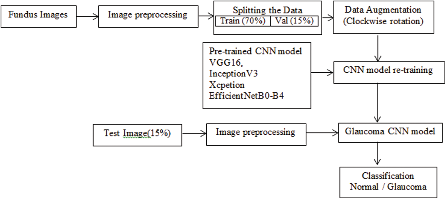
Figure 2: Block diagram of the proposed approach
This study uses a total of 2065 images in two classes, collected from public data sets RIM-ONEV2 and V3, ORIGA, DRISHTI-GS1, HRF, and ACRIMA. The size of each RGB fundus dataset varies. The statistics of RGB images collected from different datasets have shown in Tab. 1. The rotation augmentation techniques have been used on each image of the datasets to improve the experimental data series quality upto 10325 images and avoid model overfitting. The number of images increases by rotating the images in a clockwise direction from 0o to 4o.
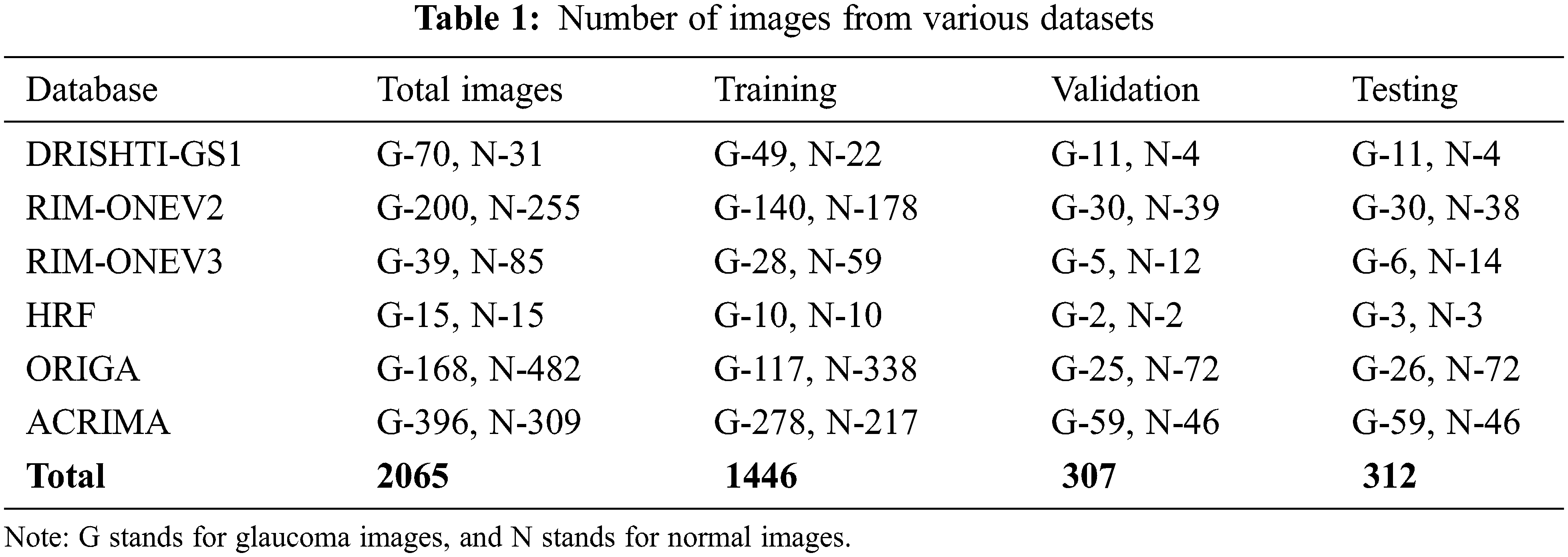
DRISHTI–GS1 database, published by Aravind Eye Hospital, Madurai, contain 101 optic disk-centered fundus images and is captured with the field of view of 300. Four experts categorized the images into 89 glaucoma images and 12 normal images. The ORIGA database comprised 168 Glaucoma and 482 normal images and had annotated by well-trained Singapore Eye Research Institute professionals. Three Spanish hospital collaborations produced RIM-ONEV2 & V3 with all images focused on an optical disc. RIM-ONEV2 contains 200 images of Glaucoma and 255 normal images. RIM-ONEV3 includes 85 normal images and 39 Glaucoma images. Four glaucoma experts had annotated all images. The database ACRIMA includes 309 Non-Glaucoma, and 396 Glaucoma images had obtained from ACRIMA project. Most of the fundus images are centered OD with 350 fields of view. Two ophthalmologists with eight years of experience provided an annotation of fundus images. A collaborative research group established High-Resolution Fundus (HRF) image databases which contain 15 healthy and Glaucoma images, respectively. A group of experts and ophthalmologists generates the golden standard data. Fig. 3 shows a few sample fundus images of various datasets.
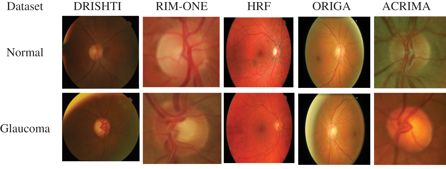
Figure 3: Sample fundus images from various datasets
3.2 Proposed CNN Models with Transfer Learning
The proposed work implements transfer learning on eight different CNN models. We freeze all models layers and train only the top layers with a significant learning rate as the first step of transfer learning. Next, we unfreeze the top layers while leaving BatchNorm layers frozen with a lower learning rate to accelerate the training. The binary classification (normal and Glaucoma) obtains by adding a softmax layer at the network’s end. We use a suitable optimizer for CNN models and a binary cross-entropy loss function to train the models. We selected commonly used architectures like VGG16, Inception, Xception, and the recently proposed EfficientNet. We conducted several experiments to analyze the performance of the selected architecture, fine-tuning verse full training. We present the details of the network used for glaucoma classification.
VGG16 has sixteen layers which ILSVRC-2014 has won with a parameter of around 138 million and structured with identical convolution layers, same padding, and max-pooling layers using 3 × 3 filters with stride 1, 2 × 2 filters with stride 2 [31]. The thirteen layers of convolution and max-pooling have consistently organized throughout the VGG16 architecture. First, the input layer takes image size as 224 × 224 pixels. Last, it contains fully connected layers with two ReLU and softmax activation functions.
The architecture of an InceptionV3 network has progressively been built by Google [32]. In addition to older versions, the factorized convolution benefits to decrease the network parameters, i.e., smaller convolution, leads to faster training. A 3 × 3 convolution is replaced by a 1 × 3, followed by a 3 × 1 convolution called Asymmetric convolutions. An Auxiliary classifier inserts where it acts as a regularizer and pooling operation done by grid size reduction. InceptionV3 has symmetric and asymmetric convolution blocks, an average pooling, maximum pooling, concats, dropouts, and fully connected layers. The InceptionV3 consists of 42 layers; the image size is 299 x 299 pixels for the input layer, fully connected layers addedat the end of inception, and softmax layer at last for glaucoma classification.
Xception [33] suggested another CNN model, which stands for Extreme Inception. This CNN architecture entirely depends on depth-wise separable convolution layers, and cross-channel correlation and spatial correlations mapping have completely uncoupled on CNN feature maps. Xception’s architecture has 36 convolution layers which form the network’s base for feature extraction. A logistic regression layer follows a convolution layer and inserts a fully connected layer before the logistical regression layer. All 14 modules had linked to linear residual connections except for the first and last modules. In short, a linear stack of depth-wise separable convolution layers with residual connection is an Xception architecture.
“Google AI suggests a more efficient method, as its name suggests, while improving progress by achieving 84.4% accuracy at 66 million parameters in the problem of ImageNet classification” [34]. The network dimensions of the model are structure as width, depth, and resolution, and that has uniformly scaled in a more principled way, i.e., the accuracy with a fixed set of scaling coefficients has increased gradually. Instead of a Rectifier Linear Unit (ReLU), this model uses a Swish activation function. The EfficientNet CNNs have structured with a compound coefficient. The grid search takes place as the first step in compound scaling to find a relation between the various scale dimensions of the baseline network under a constraint of fixed resources. It defines the appropriate scaling coefficient to scale the primary network to the desired target size for depth, width, and resolution measurements [34].
The EffiicientNet architecture has been used mobile inverted bottleneck convolution (MBConv) as the main building block similar to MobileNetV2 [35]. Still, it is slightly oversized due to an increase in the FLOP budget. At first, the MBConv maps were first expanded to 1 × 1 convolutions to improve the depth of the feature map. The 3 × 3 deep convolutions and points-wise convolutions reduce the number of output feature map channels. The shortcut between the bottlenecks has been connected to a smaller number of channels, whereas skip connections formed the wider layers. An in-depth separable convolution is created to reduce kernel size by nearly k2 compared to traditional layers, and the height and width of the 2D convolution window are specified by it [35]. Fig. 4 shows the block diagram of EfficientNetB0.
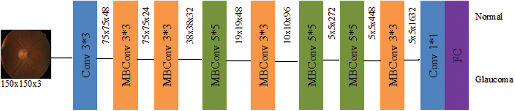
Figure 4: Schematic representation of EfficientNetB0
The compound coefficient φ has utilized principles laid down in Eq. (1) to uniformly scale up the depth, width, and resolution uniquely. The unique scaling technique is called the compound scaling process.
The constant α, β, γ determines the depth, resolution, and width of the network. For different user-defined coefficient φ value and α, β, γ as constants, a family of EfficientNet (B1-B7) has created from the baseline EfficientNetB0 network.
The proposed CNN models are implemented on the training images and evaluated on the test images, as discussed in Section 3.1. The test images consist of 151 normal and 161 glaucoma images. This section presents the performance metrics, experimental setup, training phase, and performance analysis.
The effectiveness of all CNN models is validated using the performance measures [36]. Accuracy (ACC), sensitivity (SN), specificity (SP) is the most commonly used measures for assessing the architecture performance, which utilizes the terms: False Positive (FP), False Negative (FN), True Positive (TP), and True Negative (TN) from the confusion matrix. The mathematical expressions for chosen metrics have given in Eqs. (2–4).
Compute other induces from the confusion matrix using Eqs. (5–8) that contains the F1-score, Kappa index, Final score, and precision (Pre)
where
Accuracy is first assessing index in classification problem which refers to the rate of correct classification to the proportion of the sample. Precision shows how much of the positive prediction from all positive identification has been correctly predicted. Sensitivity refers to the ratio of samples that from all true positive values are correctly predicted positive. Specificity refers to the ratio of samples from all true negatives that are correctly predicted negatives.
The model stability assesses by AUC, ROC, and also kappa score and classification accuracy. The AUC and ROC curve nearer to 1 shows the best performance in the model classification. F1_score is a harmonic average of accuracy and recall, and the score near 1 shows good model classification performance. The average of AUC, Kappa, and F1_score gives the Final score of model performance.
The first CNN for handwritten digit recognition classification is proposed by LeCun et al. [37]. CNN uses convolution and offers better performance for the segmentation and classification of images in medical imaging rather than simple matrix multiplication operations. CNN architecture composed various vital layers like convolution, batch normalizing, rectifier linear unit, fully connected, and pooling layers [38]. The VGG16, InceptionV3, Xception, and EfficientNetB0-B4 models use pre-trained weights for classification of Glaucoma instead of training the models from scratch, i.e., weights determined using the ImageNet database through CNN training. The architectures of all proposed CNNs are all implemented via the TensorFlow framework Keras packages.
The database images normalize by subtracting the average and dividing by the standard deviation computed on all the pixels of an image. Image dimensions for VGG16 were resized to 224 × 224 pixels, 299 × 299 pixels for InceptionV3 and Xception. The input image size for all EfficientNet architecture models was defined as 150 × 150 pixels by trial and error studies. The Global Average Pooling layer (GAP) has fed with feature maps extracted from CNN. The optimized final feature vector for classifying binary fundus images achieves by linking the sigmoid activation function with the binary cross-entropy loss function. Eq. (9) gives the mathematical expression for sigmoid activation function
The activated units were optimized by binary cross-entropy function using Eq. (10) that depends on labels of ground truth (y) and predicts labels (
The loss function is measured by how far the predicted value from the actual value is from each class.
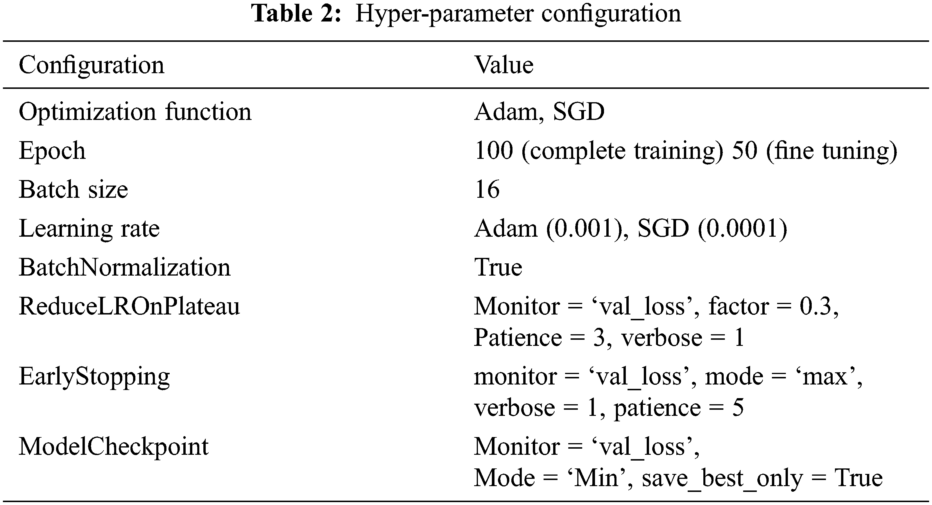
As mention in the previous section, we createa base pre-trained model for EfficientNetB0-B4, InceptionV3, Xception, and VGG16 using ImageNet. The model layers modify by adding the Global Averaging Pooling (GAP) layer and a fully connected layer with a Dense of 1024 layer to predict two output classes using softmax activation. Again tarin the top layers of a new model and compile using binary cross-entropy with Adam (Adaptive Moment Estimation) optimizer for EfficientNetB0-B4, Inception, Xception, and SGD optimizer for VGG16. Next, we freeze the bottom convolution layer of a new model and train the top five layers with a batch size of 16, the learning rate of 0.0001 for Adam, and 0.001 for SGD.The model’s hyper-parameter configuration tabulated in Tab. 2.
As mentioned earlier, training and evaluation have experimented with proposed models. The test fundus images contain 312 patients’ images and contain no ground truth. The test images were predicted and evaluated by saved model weight using the confusion matrix. The model performance assesses as mentioned above.
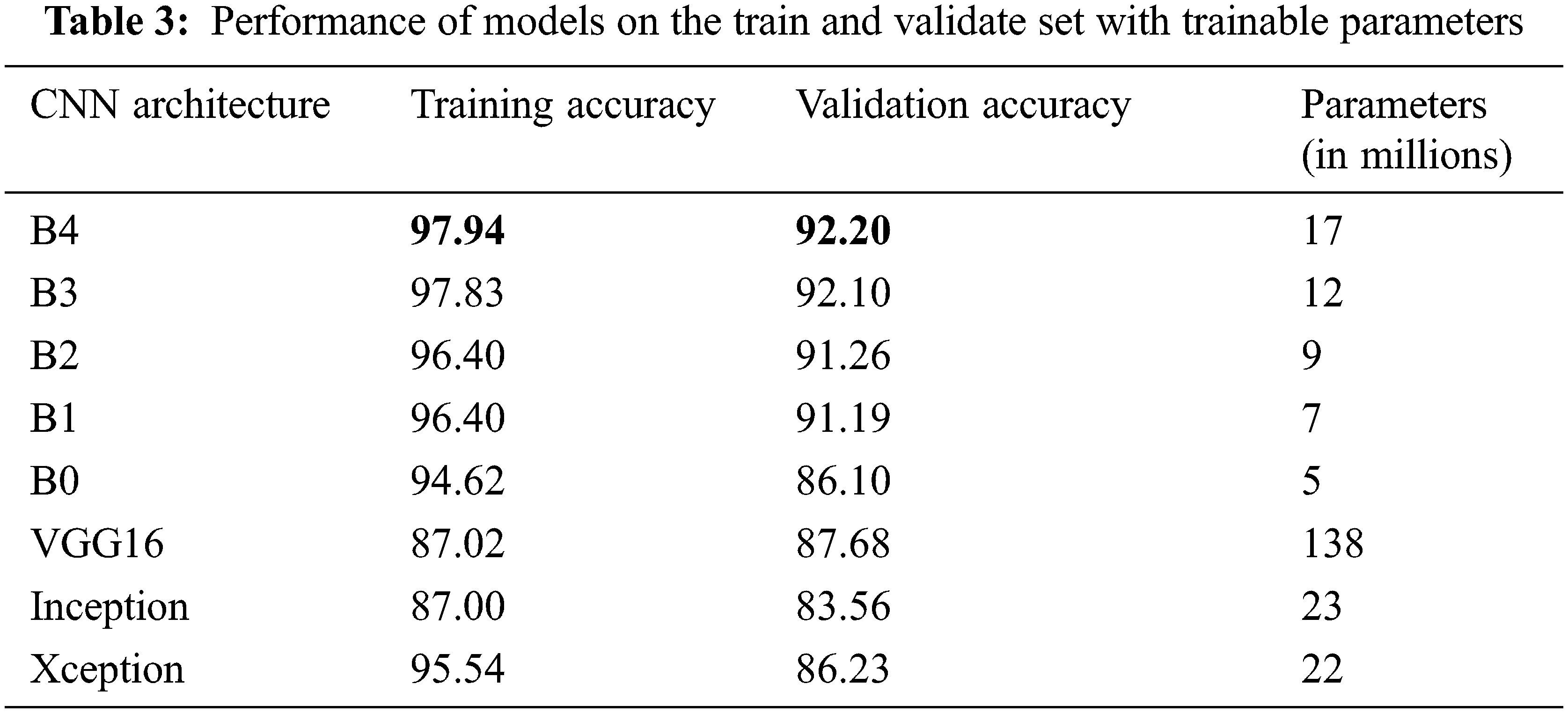
The number of trainable parameters and accuracy of each CNN architecture presents in Tab. 3. In terms of training and validation accuracy, the EfficientNet models performed better than other models such as VGG16, InceptionV3, and Xception. It is possible to see that the trainable parameters for EfficientNetB4 are much less than the VGG16 model, which requires less computation power and resources to fine-tune the EfficientNet parameters.
The training progression curve after fine-tuning the top layers for EfficientNetB4 describes in Fig. 5. It is apparent from the training and validation curve that the model reached the highest level of accuracy in 27 epochs.
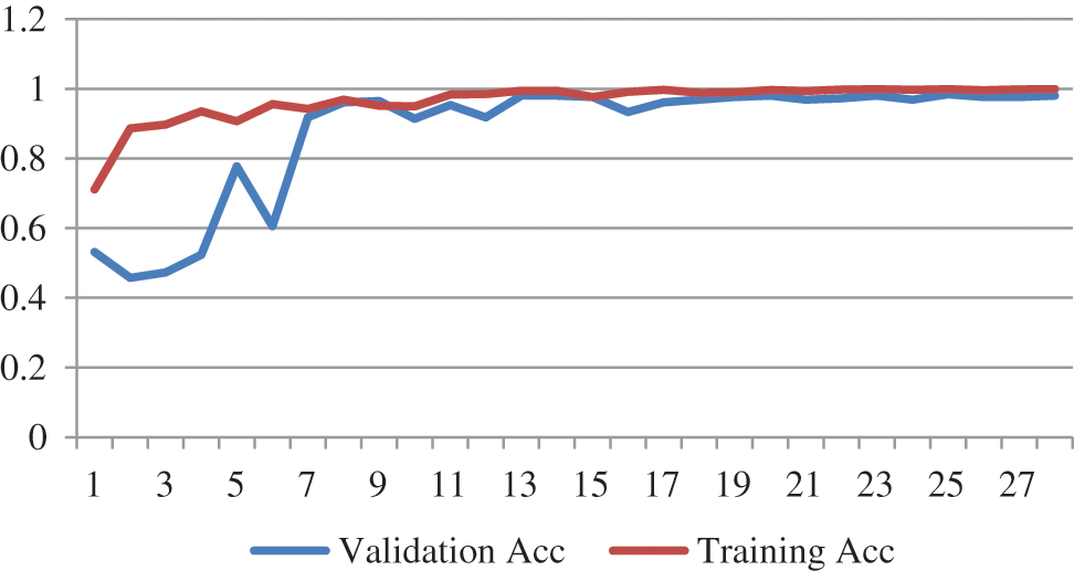
Figure 5: Training progress curve for EfficientNetB4
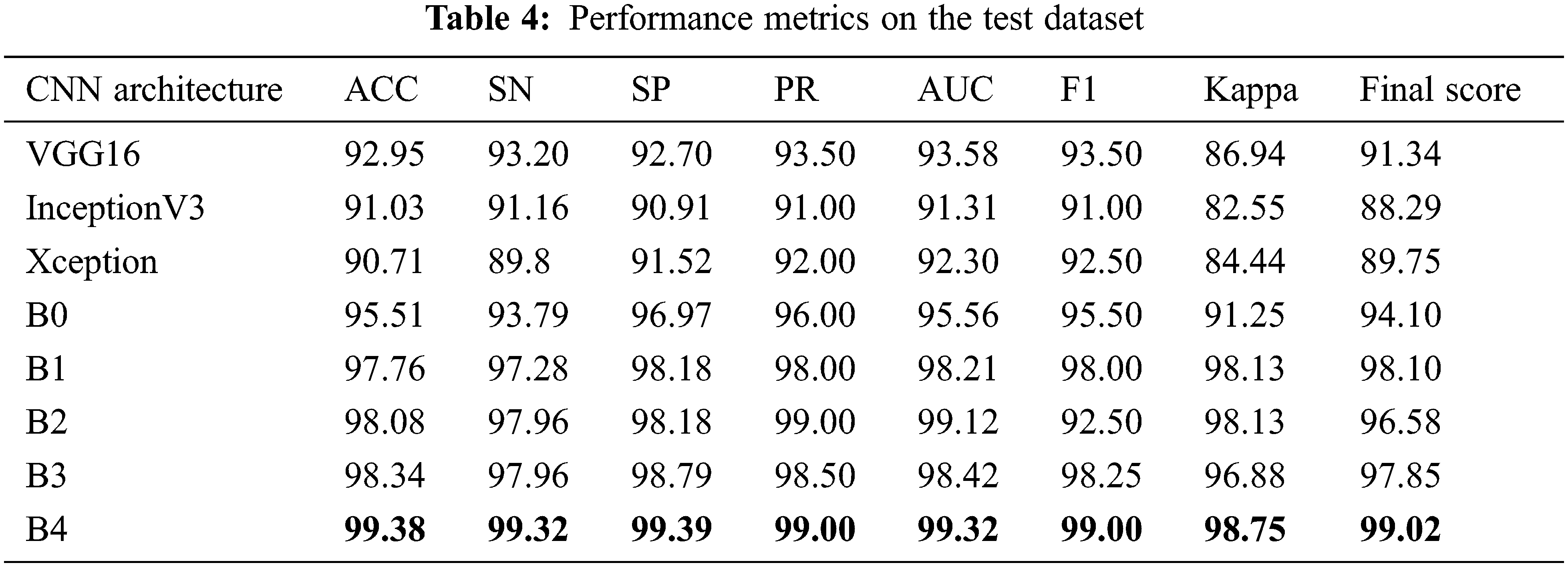
From Tab. 4, all models have accuracy, sensitivity, and specificity, ROC, AUC, F1_score, kappa, and Final score values greater than 90% of each other. However, compared to all other architectures, the results showed EfficientNetB4 as the best performance. We found that the EfficientNetB4 models’ sensitivity and specificity values are higher than the other models for class prediction. The actual rates of classification for EfficientNetB4 model samples are higher than the other models that are elsewhere. For Glaucoma, our deep learning model achieves 99.38% accuracy, 99.32% sensitivity, and 99.39% specificity, and 99.32% AUC in the test set. The F1_score and kappa values are closer to 1 than the other models, indicating a better classification for the proposed deep learning model.
In addition to the measures shown in Tab. 3, ROCs results from all proposed CNN models are provided in Fig. 6. From the above table, all the fine-tuned models proposed are very efficient in the evaluation of Glaucoma. While they achieved a large area within the ROC curve, the system proposed model is outperforming with a value equal to 99.70% in this paper, and it adds up to the proper classification of test datasets by EfficientNetB4 have a high true fraction and low false positivity.
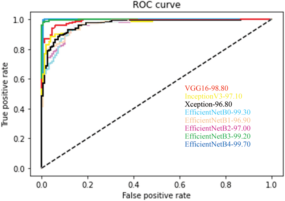
Figure 6: Average ROC for each fine-tuned CNN model
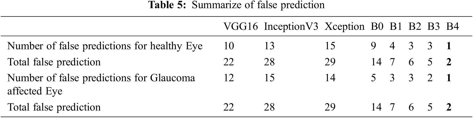
To show more clearly the performance of the architectures of the deep learning model discussed in this study. The total erroneous ranking numbers for the two classes are presents in Tab. 5. As can be seen, EfficientNetB4 is the lowest error model, while other CNN architectures have a relatively large number of errors classifications.
The final layer of the proposed model uses to construct activation maps using Grad-Cam visualization [39], highlighting the optic nerve head region in the fundus image responsible for the classification. This explainability algorithm applies to visualize the critical features according to two classes. The optic nerve head region highlighted by red for well-classified images shows in Fig. 7. In Figs. 7 & 8, the classification results obtained from the EfficienrNetB4 model and heatmaps generated using features of the last layer are presented for correct and incorrect classification.
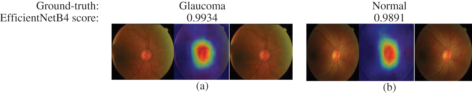
Figure 7: Samples of well-classified glaucoma and normal images by EfficientNetB4 with class activation map
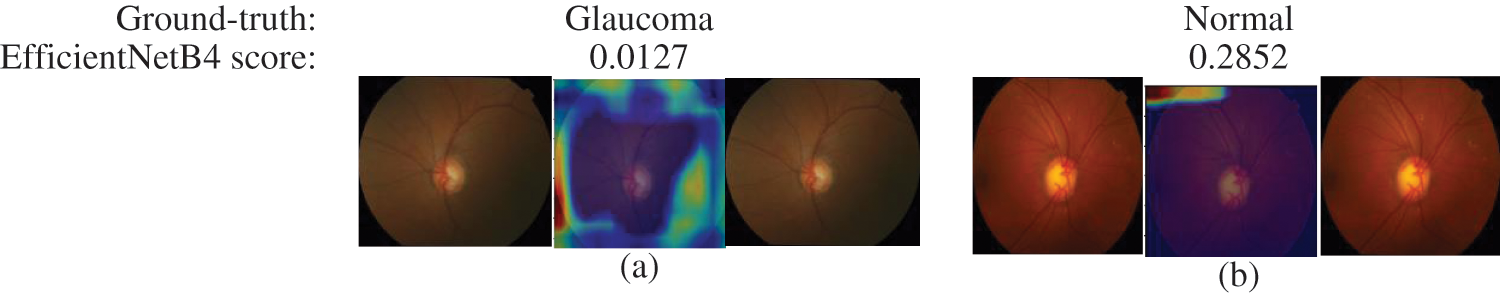
Figure 8: Samples of miss-classified glaucoma and normal images by EfficientNetB4 with class activation map
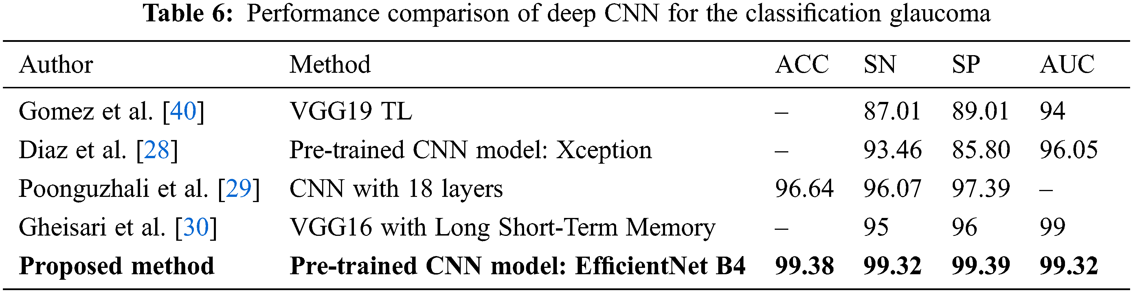
The performance comparison with the latest state-of-the-art methods using deep learning presents in Tab. 6 for Glaucoma detection on globally available and private datasets. As we can see, our proposed model outperforms the model proposed by Gomez et al. [40]. They evaluated the model’s performance by incorporating the clinical history of data and tonometry tests with the fundus images for the total test dataset and observed that the sensitivity and specificity value increased slightly withthe same AUC of 0.94. Compared to Quigley et al. [3], the proposed model performs better with around 17 million trainable parameters. And also, our model has a high-performance score compared to Raghavendra et al. [26]. For ACRIMA, an accuracy of 96.64% is the best result presented in their work and an analysis of the classification accuracy by adding noise to the database. Gheisari et al. [30] also considered the problem of classifying Glaucoma by using fundus images as well as sequence images. They obtained an AUC score of 0.99, close to our score of 0.9932, with an image size of 150 x 150 pixels. Still, our model achieves a better specificity and sensitivity compared to Gheisari et al. [30].
This study highlighted deep learning methods for detecting Glaucoma from images of the fundus. The fine-tuning process applies to all models for the detection of Glaucoma. The metric values of the EfficientNetB4 model outperform using public datasets. The performance of the CNN models is evaluated through different metrics like sensitivity, precision, specificity, accuracy, ROC, AUC, F1_score, kappa, and Final score. Experimental results show that a higher accuracy of 99.38% has been achieved for the EfficientNetB4 model, as described elsewhere. In a word, the EfficientNetB4 model may be considered the best model for identifying signs of Glaucoma. The adaption of the model to assess the severity level of Glaucoma and the classification of other types of retinal diseases may be considered.Regardless, the proposed automatic Glaucoma detection systems have some limitations in the performance due to different labeling standards used in publicly available datasets and the quality of the images.
Acknowledgement: The authors would like to express their sincere thanks to the journal editorial committee members, reviewers, and Head of the EEE department of National Engineering College for the valuable suggestions to improve the paper.
Funding Statement: The authors received no specific funding for this study.
Conflicts of Interest: The authors declare that they have no conflicts of interest to report regarding the present study.
1. D. Pascolini and S. P. Mariotti, “Global estimates of visual impairment: 2010,” British Journal of Ophthalmology, vol. 96, no. 5, pp. 614–618, 2015. [Google Scholar]
2. R. R. A. Bourne, S. R. Flaxman, T. Braithwaite, M. V. Cicinelli, A. Das et al., “Magnitude, temporal trends, and projections of the global prevalence of blindness and distance and near vision impairment: A systematic review and meta-analysis,” Lancet Global Health, vol. 5, no. 9, pp. 888–897, 2017. [Google Scholar]
3. H. Quigley and A. T. Broman, “The number of people with glaucoma worldwide in 2010 and 2020,” British Journal of Ophthalmology, vol. 90, no. 3, pp. 262–267, 2006. [Google Scholar]
4. Y. C. Tham, X. Li, T. Y. Wong, H. A. Quigley, T. Aung et al., “Global prevalence of glaucoma and projections of glaucoma burden through 2040: A systematic review and meta-analysis,” Ophthalmology, vol. 121, no. 11, pp. 2081–2090, 2014. [Google Scholar]
5. P. Jyotika, K. Kavita and S. Arora, “Optic cup segmentation from retinal fundus images using glow worm swarm optimization for glaucoma detection,” Biomedical Signal Processing & Control, vol. 60, pp. 1–12, 2020. [Google Scholar]
6. M. D. Abramoff, M. K. Garvin and M. Sonka, “Retinal imaging and image analysis,” IEEE Reviews in Biomedical Engineering, vol. 3, pp. 169–208, 2010. [Google Scholar]
7. M. Singh, M. Singh and J. K. Virk, “Glaucoma detection techniques: A review,” Computer Science & Electronics Journals, vol. 6, no. 2, pp. 66–76, 2015. [Google Scholar]
8. D. W. K. Wong, J. Liu, J. H. Lim, X. Jia, F. Yin et al., “Level-set based automatic cup-to-disc ratio determination using retinal fundus images in ARGALI,” in Proc. IEMBS, Vancouver, BC, Canada, pp. 2266–2269, 2008. [Google Scholar]
9. K. Thakkar, K. Chauhan, A. Sudhalkar and R. Gulati, “Detection of glaucoma from retinal fundus images by analysing ISNT measurement and features of optic cup and blood vessels,” International Journal of Engineering Technology Science & Research, vol. 4, no. 7, pp. 2394–3386, 2017. [Google Scholar]
10. F. A. Medeiros, L. M. Zangwill, C. Bowd, R. M. Vessani, R. Susanna et al., “Evaluation of retinal nerve fiber layer, optic nerve head, and macular thickness measurements for glaucoma detection using optical coherence tomography,” American Journal of Ophthalmology, vol. 139, no. 1, pp. 44–55, 2005. [Google Scholar]
11. J. B. Jonas, M. C. Fern’andez and G. O. H. Naumann, “Glaucomatous parapapillary atrophy: Occurrence and correlations,” JAMA Ophthalmology, vol. 110, no. 2, pp. 214–222, 1992. [Google Scholar]
12. J. Cheng, J. Liu, Y. Xu, F. Yin, D. W. K. Wong et al., “Superpixel classification based optic disc and optic cup segmentation for glaucoma screening,” IEEE Transactions on Medical Imaging, vol. 32, no. 6, pp. 1019–1032, 2013. [Google Scholar]
13. G. D. Joshi, J. Sivaswamy and S. R. Krishnadas, “Optic disk and cup segmentation from monocular color retinal images for glaucoma assessment,” IEEE Transaction on Medical Imaging, vol. 30, no. 6, pp. 1192–1205, 2011. [Google Scholar]
14. F. Yin, J. Liu, D. W. K. Wong, N. M. Tan, C. Cheung et al., “Automated segmentation of optic disc and optic cup in fundus images for glaucoma diagnosis,” in Proc.CBMS, Rome, Italy, pp. 1–6, 2012. [Google Scholar]
15. A. D. Pinto, S. Morales, V. Naranjo, P. Alcocer and A. Lanzagorta, “Glaucoma diagnosis by means of optic cup feature analysis in color fundus images,” in Proc. EUSIPCO, Honolulu, HI, USA, pp. 2055–2059, 2016. [Google Scholar]
16. R. Bock, J. Meier, L. G. Nyúl, J. Hornegger and G. Michelson, “Glaucoma risk index: Automated glaucoma detection from color fundus images,” Medical Image Analysis, vol. 14, no. 3, pp. 471–481, 2010. [Google Scholar]
17. N. Srivastava, G. Hinton, A. Krizhevsky, I. Sutskever and R. Salakhutdinov, “Dropout: A simple way to prevent neural networks from overftting,” Journal of Machine Learning Research, vol. 15, no. 56, pp. 1929–1958, 2014. [Google Scholar]
18. O. Russakovsky, J. Deng, H. Su, J. Krause, S. Satheesh et al., “ImageNet large scale visual recognition challenge,” International Journal of Computer Vision, vol. 115, no. 3, pp. 211–252, 2015. [Google Scholar]
19. G. Carneiro, J. Nascimento and A. P. Bradley, “Unregistered multiviewmammogram analysis with pre-trained deep learning Models,” in Proc.MICCAI, Munich, Germany, pp. 652–660, 2015. [Google Scholar]
20. H. Chen, D. Ni, J. Qin, S. Li, X. Yang et al., “Standard plane localization in fetal ultrasound via domain transferred deep neural networks,” IEEE Journal of Biomedical & Health Informatics, vol. 19, no. 5, pp. 1627–1636, 2015. [Google Scholar]
21. N. Tajbakhsh, J. Y. Shin, S. R. Gurudu, R. T. Hurst, B. C. Kendall et al., “Convolutional neural networks for medical image analysis: Full training or fine tuning,” IEEE Transactions on Medical Imaging, vol. 35, no. 5, pp. 1299–1312, 2016. [Google Scholar]
22. Y. Bar, I. Diamant, L. Wolf and H. Greenspan, “Deep learning with non-medical training used for chest pathology identification,” in Proc. SPIE Medical Imaging 2015, Orlando, Florida, United States, pp. 94140V, 2015. [Google Scholar]
23. A. S. Razavian, H. Azizpour, J. Sullivan and S. Carlsson, “CNN features off-the-Shelf: An astounding baseline for recognition,” in Proc. CVPRW, Columbus, OH, USA, pp. 512–519, 2014. [Google Scholar]
24. X. Chen, Y. Xu, D. W. K. Wong, T. Y. Wong and J. Liu, “Glaucoma detection based on deep convolutional neural network,” in Proc. EMBC, Milan, Italy, pp. 715–718, 2015. [Google Scholar]
25. Q. Abbas, “Glaucoma-deep: Detection of glaucoma eye disease on retinal fundus images using deep learning,” International Journal of Advanced Computer Science & Applications, vol. 8, no. 6, pp. 41–45, 2017. [Google Scholar]
26. U. Raghavendra, H. Fujita, S. V. Bhandary, A. Gudigar, J. H. Tan et al., “Deep convolution neural network for accurate diagnosis of glaucoma using digital fundus images,” Information Sciences: An International Journal, vol. 144, no. 29, pp. 41–49, 2018. [Google Scholar]
27. M. N. Bajwa, M. I. Malik, S. A. Siddiqui, A. Dangel, F. Shafait et al., “Two-stage framework for optic disc localization and glaucoma classification in retinal fundus images using deep learning,” BMC Medical Informatics & Decision Making, vol. 10, no. 136, pp. 1–16, 2019. [Google Scholar]
28. A. D. Pinto, S. Morales, V. Naranjo, T. Köhler, M. J. Mossi et al., “CNNs for automatic glaucoma assessment using fundus images: An extensive validation,” BioMedical Engineering OnLine, vol. 18, no. 29, pp. 1–19, 2019. [Google Scholar]
29. P. Elangovan and M. K. Nath, “Glaucoma assessment from color fundus images using convolutional neural network,” International Journal of Imaging Systems & Technology, vol. 31, no. 2, pp. 955–971, 2020. [Google Scholar]
30. S. Gheisari, S. Shariflou, J. Phu, P. J. Kennedy, A. Agar et al., “A combined convolutional and recurrent neural network for enhanced glaucoma detection,” Scientific Reports, vol. 11, no. 1, pp. 1–11, 2021. [Google Scholar]
31. K. Simonyan and A. Zisserman, “Very deep convolutional networks for large-scale image recognition,” arXiv preprint arXiv:1409.1556, 2014. [Google Scholar]
32. C. Szegedy, V. Vanhoucke, S. Ioffe, J. Shlens and Z. Wojna, “Rethinking the inception architecture for computer vision,” in Proc. CVPR, Las Vegas, NV, USA, pp. 2818–2826, 2016. [Google Scholar]
33. F. Chollet, “Xception: Deep learning with depthwise separable convolutions,” in Proc. CVPR, Honolulu, HI, USA, pp. 1800–1807, 2017. [Google Scholar]
34. M. Tan and Q. Le, “EfficientNet: Rethinking model scaling for convolutional neural networks,” in Proc. PMLR, Long Beach, California, pp. 6105–6114, 2019. [Google Scholar]
35. S. Mark, H. Andrew, Z. Menglong, Z. Andrey and C. Liang-Chieh, “Mobilenetv2: Inverted residuals and linear bottlenecks,” in Proc. CVPR, Salt Lake City, UT, USA, pp. 4510–4520, 2018. [Google Scholar]
36. J. Fan, S. Upadhye and A. Worster, “Understanding receiver operating characteristic (ROC) curves,” Canadian Journal of Emergency Medicine, vol. 8, no. 1, pp. 19–20, 2006. [Google Scholar]
37. Y. L. LeCun, Y. Bottou, P. Bengio and P. Haffner, “Gradient-based learning applied to document recognition,” Proc. IEEE, vol. 86, no. 11, pp. 2278–2324, 1998. [Google Scholar]
38. N. Gour and P. Khanna, “Multi-class multi label ophthalmological disease detection using transfer learning based convolutional neural network,” Biomedical Signal Processing and Control, vol. 66, no. 3, pp. 1–8, 2020. [Google Scholar]
39. R. R. Selvaraju, M. Cogswell, A. Das, R. Vedantam, D. Parikh et al., “Grad-CAM: Visual explanations from deep networks via gradient-based localization,” in Proc. ICCV, Venice, Italy, pp. 618–626, 2017. [Google Scholar]
40. J. J. G. Valverde, A. Anton, G. Fatti, B. Liefers, A. Herranz et al., “Automatic glaucoma classification using color fundus images based on convolutional neural networks and transfer learning,” Biomedical Optics Express, vol. 10, no. 2, pp. 892–913, 2019. [Google Scholar]
 | This work is licensed under a Creative Commons Attribution 4.0 International License, which permits unrestricted use, distribution, and reproduction in any medium, provided the original work is properly cited. |