DOI:10.32604/csse.2022.023882
| Computer Systems Science & Engineering DOI:10.32604/csse.2022.023882 | |
| Article |
Multi-Site Air Pollutant Prediction Using Long Short Term Memory
Anna University, Chennai, 600066, Tamil Nadu, India
*Corresponding Author: Chitra Paulpandi. Email: chitrapaulpandi09@gmail.com
Received: 25 September 2021; Accepted: 08 November 2021
Abstract: The current pandemic highlights the significance and impact of air pollution on individuals. When it comes to climate sustainability, air pollution is a major challenge. Because of the distinctive nature, unpredictability, and great changeability in the reality of toxins and particulates, detecting air quality is a puzzling task. Simultaneously, the ability to predict or classify and monitor air quality is becoming increasingly important, particularly in urban areas, due to the well documented negative impact of air pollution on resident’s health and the environment. To better comprehend the current condition of air quality, this research proposes predicting air pollution levels from real-time data. This study proposes the use of deep learning techniques to forecast air pollution levels. Layers, activation functions, and a number of epochs were used to create the suggested Long Short-Term Memory (LSTM) network based neural layer design. The use of proposed Deep Learning as a structure for high-accuracy air quality prediction is investigated in this research and obtained better accuracy of nearly 82% compared to earlier records. Determining the Air Quality Index (AQI) and danger levels would assist the government in finding appropriate ways to authorize approaches to reduce pollutants and keep inhabitants informed about the findings.
Keywords: LSTM; epochs; deep learning; air quality index; particulates; neural networks
It is due of air that we are living today. Every month, we breathe roughly 1 million times without realizing the consequences of the air pollution we inhale. Over 93 percent of the world’s population is exposed to dangerous air pollution chemicals such as Nitrogen Oxides (NOx), Carbon Oxides (COx), Sulphur Oxides (SOx), Particulate Matter (PM), Ozone (O3), and Ammonia (NH3) on a daily basis. Indoor air pollution is also much worse than outdoor pollution. Everyday products contain toxic compounds.
Noise, land, water, and air pollution are all major pollutants that influence humans and other living things. Among the several types of pollution, air pollution is the most serious. Natural disasters, automobiles, industries, crop fires, dust storms, man-made smokes such as burning of wood, plastics, natural gas, and coal, deforestation, population, and other factors all contribute to air pollution in India and is typically lower in summer than in the winter. Air pollution increases the risk of a variety of health problems, including arrhythmia, ischemia, heart failure, and stroke and so understanding and monitoring air pollution is critical for our well-being. The government employs the Air Quality Index (AQI) concept to forecast air pollutant levels and inform citizens.
AQI is a tool that displays the current state of air quality in six categories based on ambient concentration levels of air contaminants. Good, satisfactory, moderate, poor, very poor, and severe are the six classifications. An increase in the AQI level implies that there is a chance of breathing polluted air, which can have serious health consequences. The AQI is calculated using eight primary pollutants: Particulate Matter less than 2.5 microns (PM2.5), Particulate Matter less than 10 microns (PM10), Nitrogen Dioxide (NO2), Sulfur Dioxide (SO2), Carbon Monoxide (CO), O3, NH3, and Lead (Pb). “When we have high moisture then the aerosols in the air starts to absorb water vapors and swell thereby leads to low visibility and that is how the smog are created”, said by Sachin Ghude, Scientist, Indian Institute of Tropical Meteorology (IITM), which operates System of Air Quality Weather Forecasting and Research (SAFAR), so it is very important to forecast air pollutants for better life.
Many air pollutant studies involve knowledge of environmental and computer technology, which is time consuming, and many statistical methods such as multiple linear regression [1], auto regressive moving average method and generalized line regression [2] are used for air quality predictions [3]. When compared to traditional methods such as support vector machine [4] and random forest, a commonly used air pollution prediction method in environmental or atmospheric research performed better [5–7]. In making atmospheric decisions, accurate forecasting in air quality measurement is critical [8]. Air pollutants are also highly dependent on regional and seasonal fluctuations, making it difficult to anticipate Air Quality (AQ) and necessitating simultaneous monitoring of time and space.
Currently, the rising technology Artificial Intelligence (AI) is being employed in air pollution prediction, with advanced artificial intelligence approaches achieving improved results. Also AI founds to be the future promising technology that serves faster with more accuracy in short span of time without human intervention. Advanced AI creates great impact in several applications and improves people’s lives by performing most typical tasks. Deep Recurrent Neural Network (DRNN) is utilized in predicting fine PM2.5 [9]. Hybrid model spatiotemporal forecasting of PM2.5 is employed by long term prediction [10] and air pollutant concentration is predicted by combining other traditional methods [11,12]. Extraction of spatiotemporal characteristics improves the air pollution prediction model [13–16]. Aggregated Long Short Term Memory (LSTM) is also employed for air quality prediction [17]. Some methods provide average air pollutant concentration and to overcome the issue LSTM with Recurrent Neural Network (RNN) and Wireless Sensor Network (WSN) is employed [18]. Bayesian model [19] and bi-directional LSTM model [20] also helps to predict air quality and found to be better compared to traditional methods.
To forecast air pollution concentrations, this research proposes a deep learning model based on LSTM. Meteorological observations are obtained from a multi-site network of monitoring stations, and missing values are rebuilt and forecast values fine-tuned to make considerable improvements. The proposed model’s accuracy was improved in an experimental situation by using a real-time air pollution dataset. In addition, the suggested Deep Learning (DL) model provides accurate assessment of AQI when compared to existing methodologies, and a greater number of features were compared for air quality forecasts and accuracy in the proposed DL method, so the public is warned.
The suggested method begins with the selection of a data gathering region from local and near stations, collection of data from National Air Quality Index (NAQI), Central Pollution Control Board (CPCB), Tamil Nadu Pollution Control Board (TNPCB) and KAGGLE followed by pre-processing of data such as data division, manipulating missing data and normalization. The pre-processed data is classified using LSTM to anticipate air pollution with pinpoint accuracy. The methodology’s flow is depicted in Fig. 1:
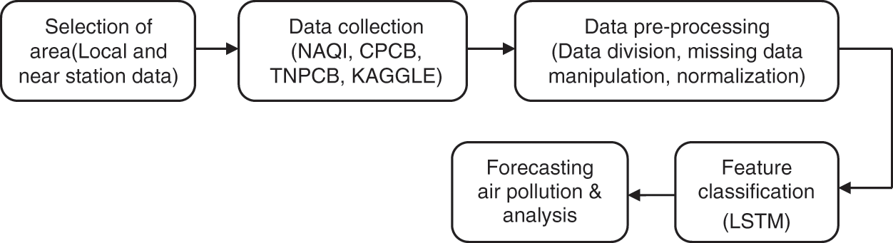
Figure 1: Process of methodology
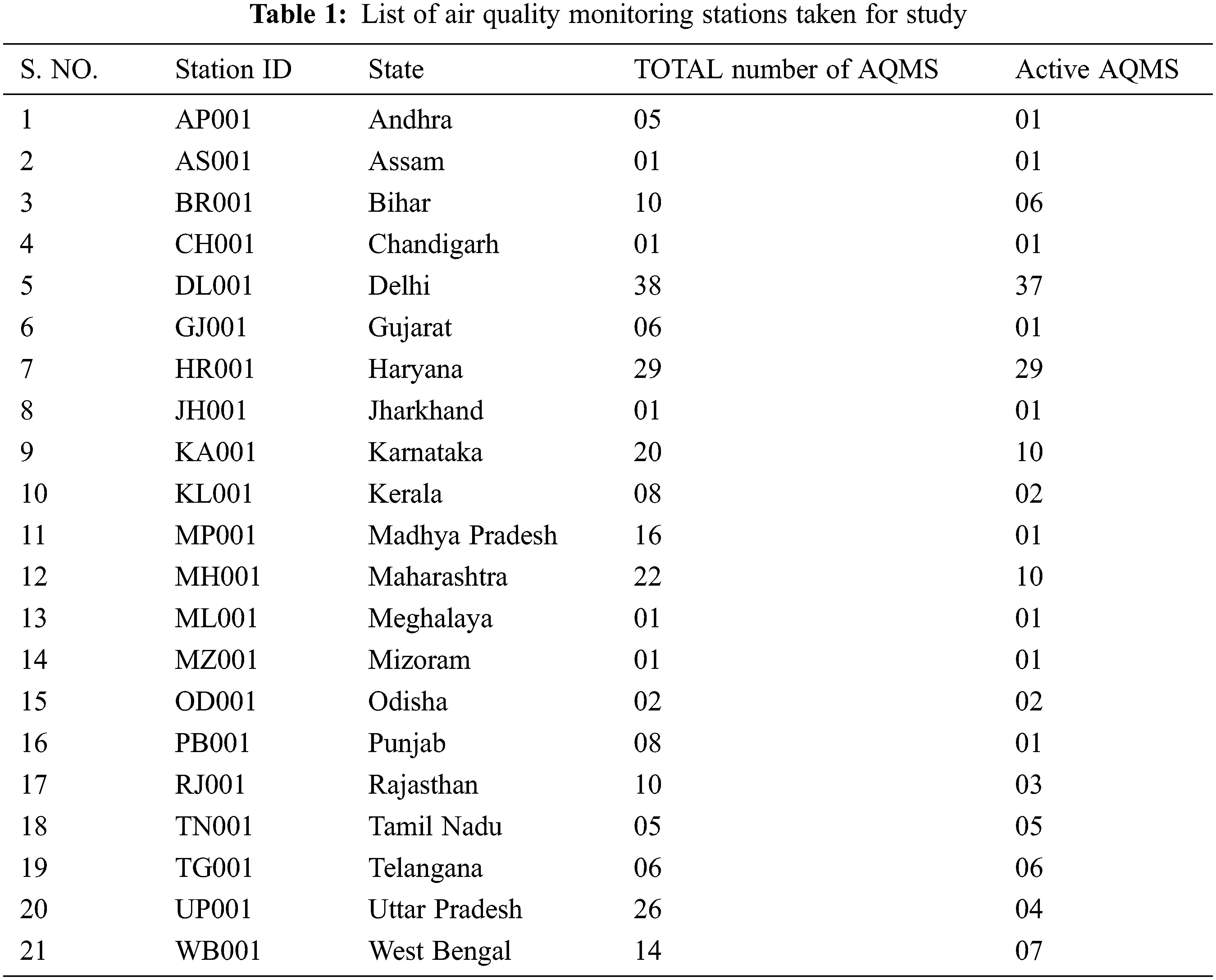
The research’s study area was gathered from Air Quality Monitoring Stations (AQMS) in the states listed in Tab. 1. For data gathering, active stations were segregated. These study sites were chosen based on the availability of CPCB air quality data, satellite images, and the fact that the areas chosen were the most polluted, trafficked, and prone to industrial development activities. Some states have inactive AQMS and so they are identified first before selecting the sites. States having active air monitoring stations details are isolated. For the planned job, the network was trained using AQMS from various states across the country. The proposed paper focus on overall air pollution prediction of the country which can further be narrowed to particular state or city area. In our study nearly 21 states are selected for experiment.
The features to be collected from the specific site are processed once the study area has been established. It is critical to comprehend the data in order to recognize the features. As a result, self-reviewing data is required, and it is assessed for all of the chosen states or cities. Fig. 2 shows a flow diagram of the data selection process.
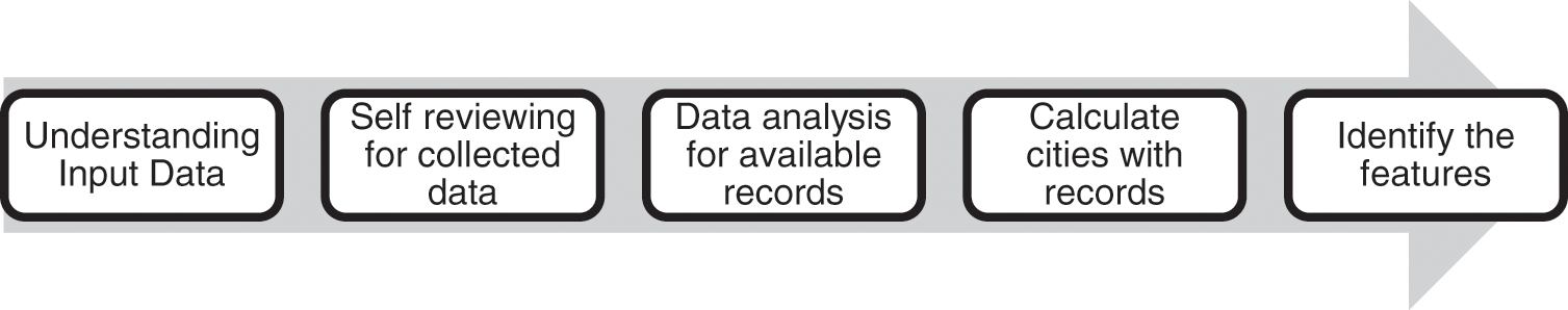
Figure 2: Process of data selection
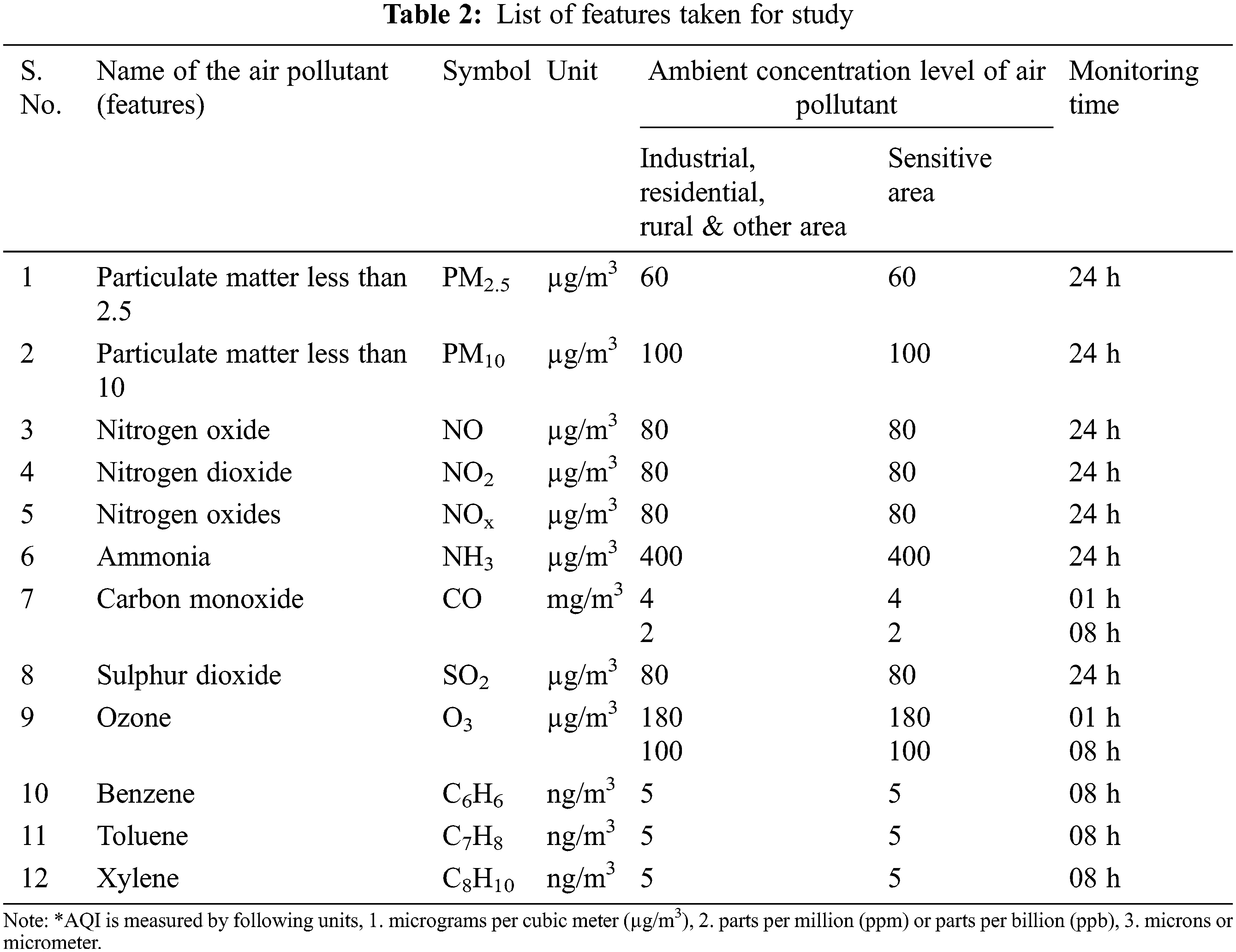
For the available number of daily Air Quality Index data per city, about 37000 records for each station are taken on an hourly basis for the specified study areas from 2016 to 2020. The data was collected for three seasons: summer, rainy season, and winter. Before preprocessing, data collected from the KAGGLE website is rigorously scrutinized. Tab. 2 lists the features that have been identified for the proposed work. It is vital to comprehend the government-mandated averaging monitoring hours and minimal ambient concentration of air pollution levels.
Once the necessary data has been gathered, it is standardized to eliminate the effects of missing numbers. Fig. 3 shows the stages involved in normalizing. Missing data is critical in preprocessing and has a significant influence on its own, thus diagnosing missing values with adequate data is critical. For these reasons, unknown values other than numbers are deleted from input data before transformation for complex numbers with a special number called Not a Number (NaN).
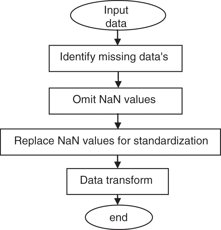
Figure 3: Input data preprocessing
For training and testing purposes, we divided the input data into two portions. Nearly 70% of the 37000 records gathered are used for training, and 30% are used for testing. Ground truth parameters are collected during training, and the network is trained using the Stochastic Gradient Descent with Momentum (SGDM) optimizer. In comparison to other current algorithms, this best approach finds the model parameters that best fit the expected and actual outputs, calculates faster, and converges better with longer training time. Before training LSTM categorization, soft max is employed for activation layer during input data testing.
2.5 Forecasting Air Pollution and Analysis
Finally, the survey data is analyzed using methods from the Statistical Package for Social Sciences (SPSS). This SPSS software suite was used to conduct a detailed analysis of the data collected. The measurements done often includes mean, median, Standard Deviation (SD), Mean Absolute Percentage Error (MAPE), Mean Square Error (MSE), Mean Absolute Error (MAE), Root Mean Squared Error (RMSE) and Mean Squared Error (MSE) helps to predict the performance level of classifier which enables to conclude AQI.
3 AQI Prediction Model Based on LSTM
Internal memory is used by the basic RNN to process the future variable sequence of inputs. Fig. 4 depicts the basic architecture of a basic RNN. Because the original RNN in our proposed model for training the dataset may not perform well for long-term reliance because it includes simple tanh in every repeating module, we employ LSTM, which is an expanded version of RNN, to overcome this issue.
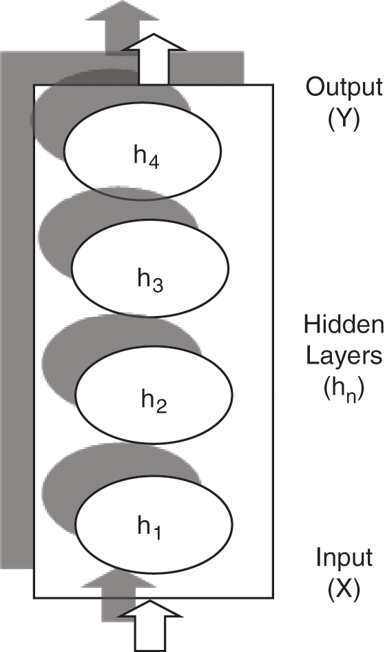
Figure 4: Basic RNN architecture
In comparison to simple RNN, the LSTM network is capable of performing long-term dependencies, which was first described by Hochreiter and Schmidhuber in 1997. It allows avoiding the long-term reliance problem. The core idea behind LSTM is as follows:
The key feature that goes horizontally through the diagram at the top is cell state. It’s similar to a conveyor belt, but with a few more interactions. This cell state can be added or withdrawn based on the information and is regulated accordingly using a three-gate structure. As shown in Fig. 5 this regulation consists of a
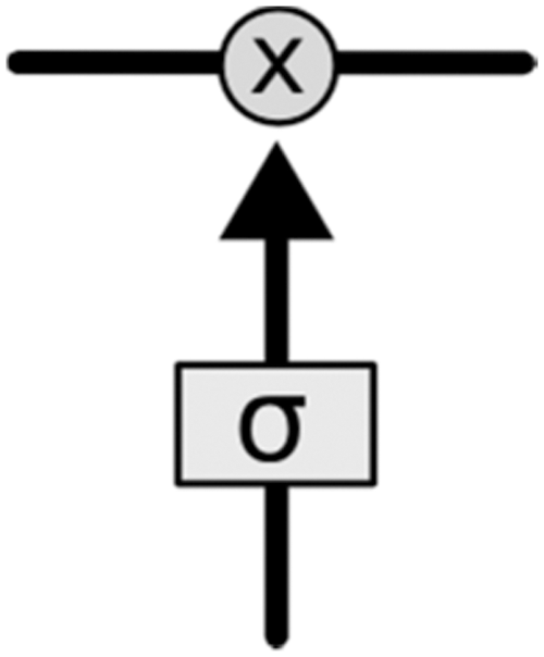
Figure 5: LSTM concept
Initially, the input data, as well as the input data concentration sequence before and after transformation, are defined. For sequence to label classification, layer array is created which includes sequence input layer, LSTM layer, fully connected layer, soft max layer and classification output layer. Sequence input layer represents total number of input features taken for study and the classes required for algorithm as decided is specified by fully connected layer. The basic block diagram of LSTM classification and regression is shown in Fig. 6:
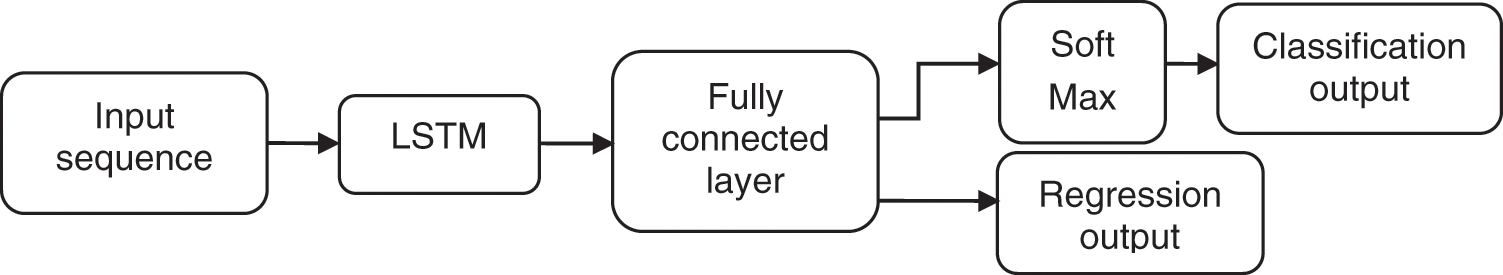
Figure 6: LSTM classification and regression
First the gender of the subject is analyzed for the given input xt and the output value ht. The sigmoid layer checks ht−1 and xt and accordingly gives the output of number between 0 and 1 for each numbers in the cell state Ct−1 as per Eq. (1). The new candidate value vector is created by tanh.
Next Ct is added to the new state followed by adding gender of the subject to the cell state as given in Eq. (2):
Now old cell state is updated Ct−1 into cell state Ct. Later forgetting of previous information is performed by multiplying ft with old state and adding it with Ct as shown in Eq. (3):
Finally the output is decided from the cell state Ct.
The LSTM starts with the details of the input data that will be given to the network, and this choice is made by a sigmoid layer dubbed the “forget gate layer” (ht−1 and xt), which produces a number between 00 and 11 for each cell state (Ct−1). The ‘input gate layer’ analyses the new information that needs to be stored in the cell state and determines which values need to be changed. The tanh layer follows the input gate, creating a vector of new added values Ct−1, which is then concatenated to provide an update to the cell state. We usually set the input values to tanh between −11 and 11 and multiply with the output sigmoid gate to only consider a certain section of the state [21].
Data collected contains some unusual or missing data and so this impact may create side effects on the whole records and so data cleaning is very important before data preprocessing. There are numerous frequent methods to replace the missing values such as mean-median of previous or next value of current data R interpolation. Data acquisition frequently involves aberrant or missing data, which might have unforeseen repercussions for the full set of records. As a result, prior to data preparation, data cleaning is essential. Missing data is removed and relevant gaps are filled in using command tools. R-interpolation, mean-median of the previous or next value of the current data is all common ways for substituting missing values. The normalized input data is shown in Tabs. 3 and 4.
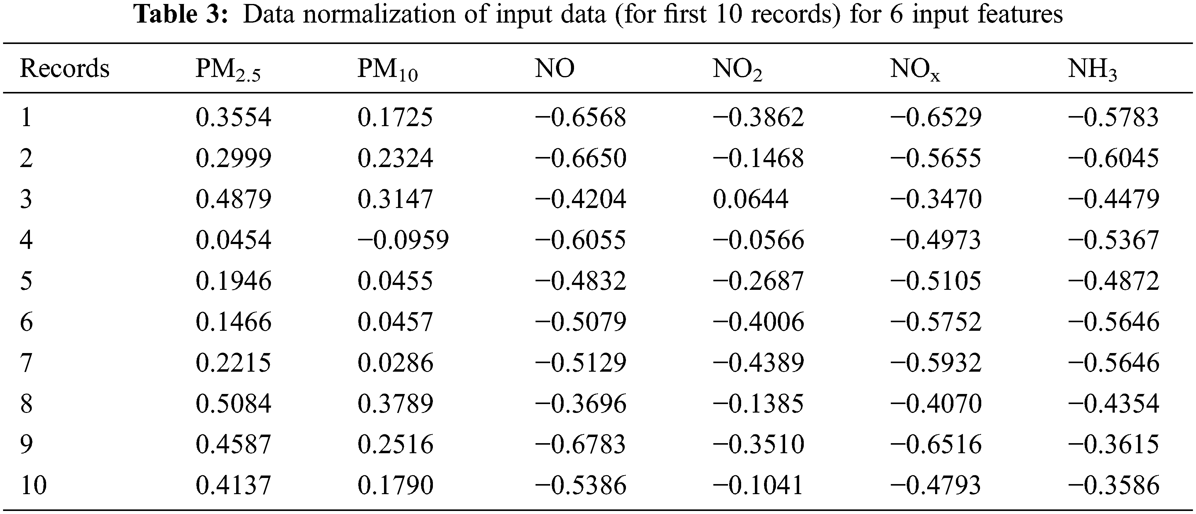
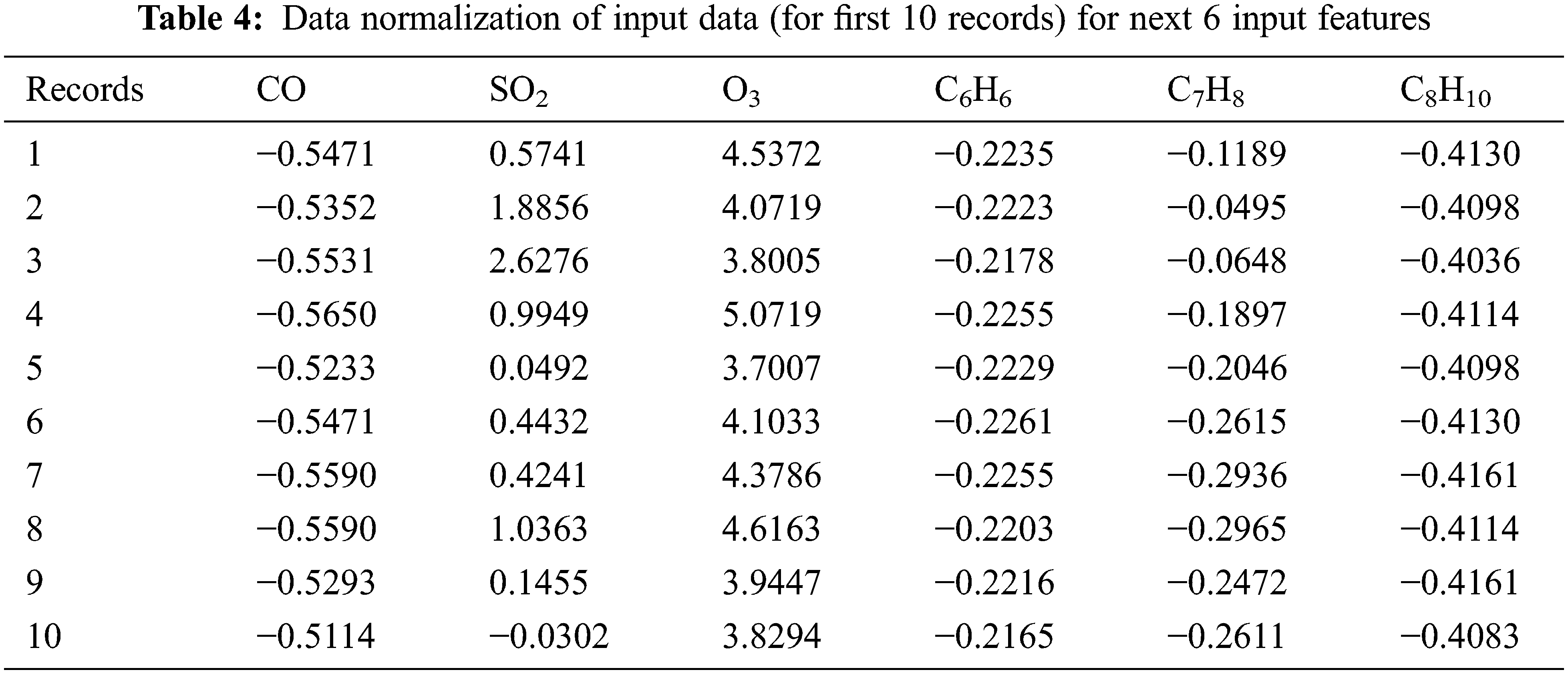
Statistical Validation of Extracted Features is done before classification, each piece of data that is used as an input must be evaluated for its importance. Tab. 5 shows the proposed characteristics and their accompanying metrics following validation. Number of samples (N), Standard Deviation (SD), Standard Error (SE), degree of freedom (df), Mean Square (MS), (measure of test accuracy) F1 Score, and significant are among the evaluation measures. The data was tested for the normality using Shapiro Walik Test and it was found that all the data was normally distributed and its significance of air pollutants is less than 0.05.
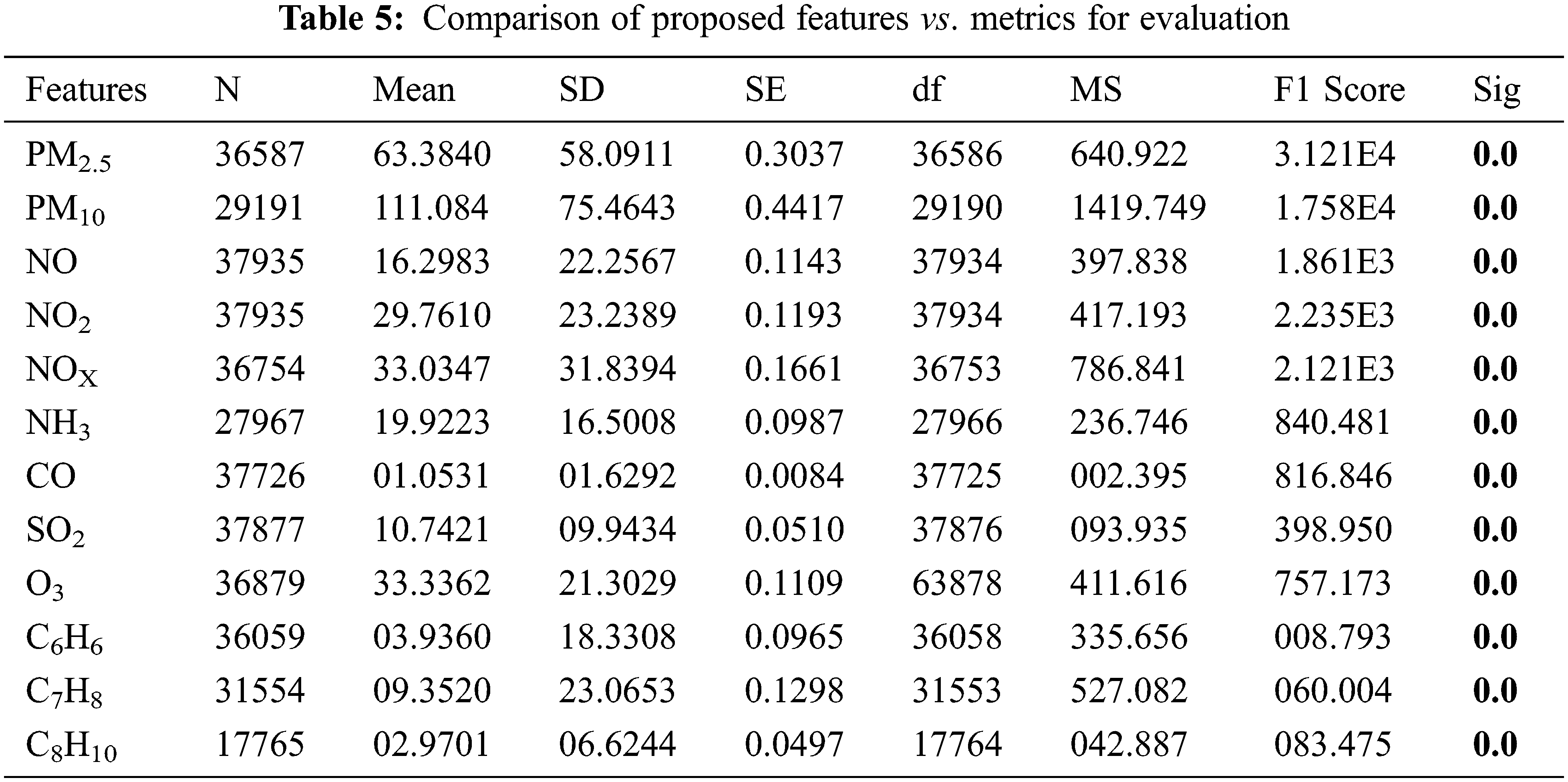
One-way Analysis of Variant (ANOVA) was used to validate the input features. It can be used for further processing if the significant value is less than 0.05. Following validation, it was determined that all of the input features used in the study were significant, implying that all of the input characteristics used in the proposed study can be used for further classification using machine learning and deep learning algorithms.
All of the significant features that have been validated using SPSS tools are used for classification. The corresponding sequence of air pollutant PM2.5 for a given set of time T is defined as X, and these values are filled with record means to get PM2.5 concentration sequence
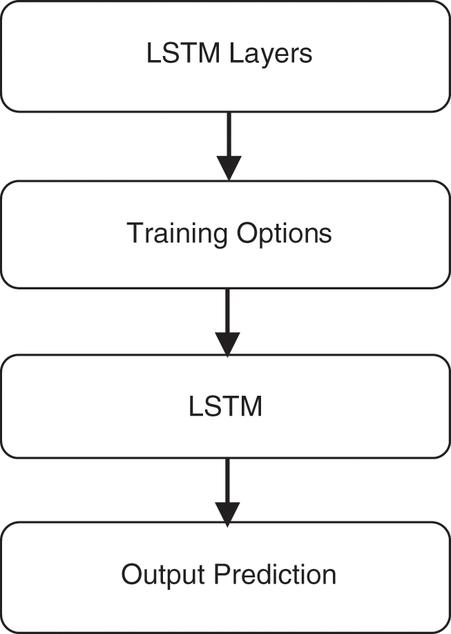
Figure 7: LSTM processing steps before network training
LSTM begins with initialization of sequence of input layers needed, fully connected layer, soft-max layer and classification layer. Then after training options are given which includes initial learning rate, (Ridge Regression) L2 regularization, drop periods, drop factors, epochs needed, batch size and SGDM. Once relevant initialization is completed then the input data’s are converted to array format and later on input and ground truth are compared in activation layer. Finally the output is predicted based on the metrics such as accuracy, precision, error rate, sensitivity, specificity, F1score.
With proper initialization of training options the network is trained for classification. Defining LSTM layers includes input sequence (fully connected layer), LSTM 120 (soft-max) and LSTM 60 (classification layer). Initialization of learning rate (0.1), L2 regularization (0.0001), schedule (piecewise), drop factor (0.1), drop period (100), maximum epochs (500), mini batch size (128), and shuffling for every epoch plots are some of the learning rate of training options.
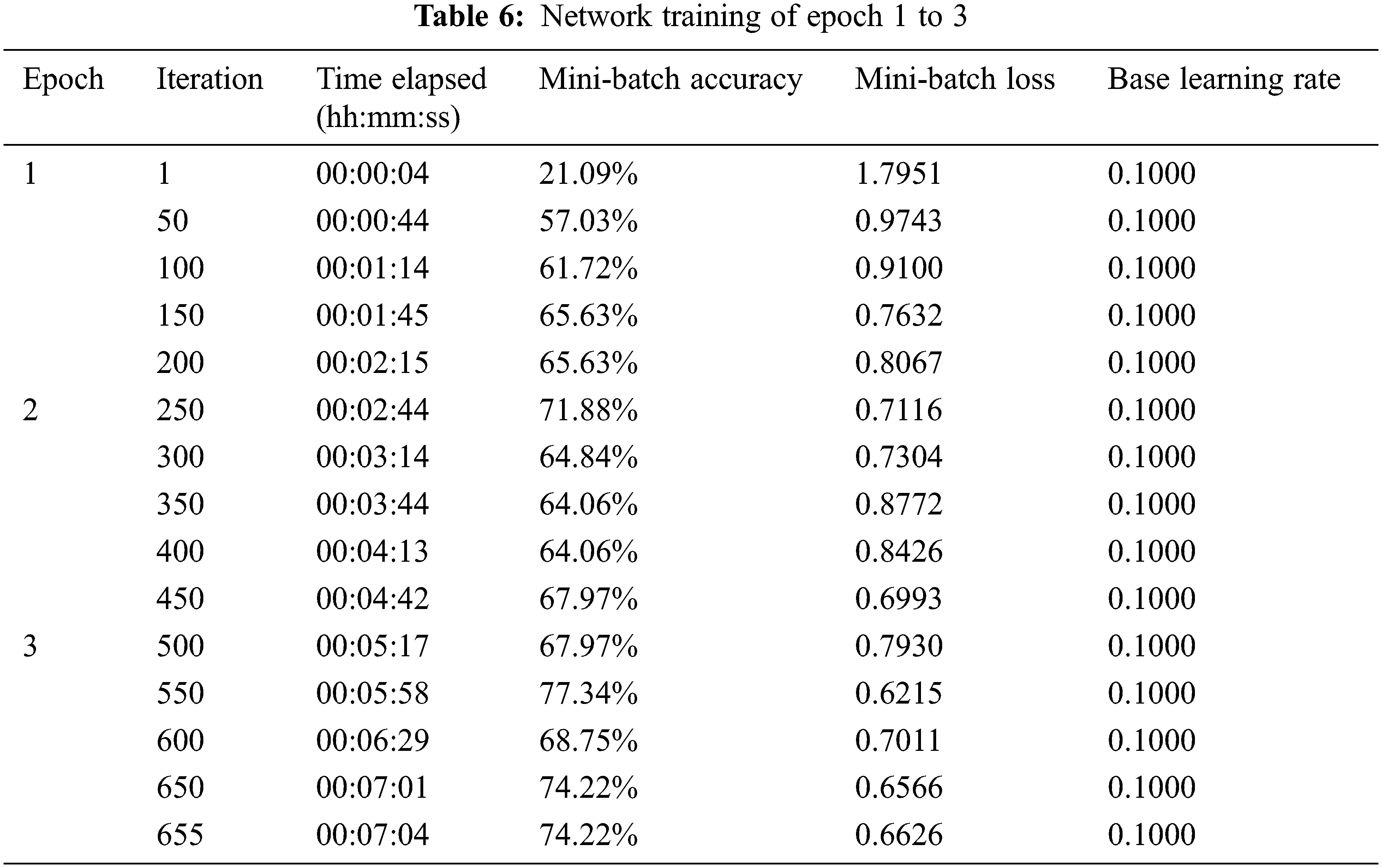
Each epoch is trained using 200 iterations, and it was discovered that the mini-batch loss and iterations are inversely proportional, with the batch loss reducing as the number of iterations grows. Tab. 6 shows the network’s initial stage of training.
The accuracy and other characteristics are assessed for various epochs after the network has been trained for the above configurations constructed according to the suggested LSTM model. Fig. 8a through Fig. 8h illustrate the relevant network training plots.
Over or under fitting can create to classification issues in a training network, hence regularisation is crucial. In machine learning, regularisation is used to solve this problem, and in deep learning, dropout regularisation is used to prevent over-fitting and under-fitting by removing random neurons from hidden layers. For large data sets hold-out validation works good compared to cross-out validation.
In general, having too many epochs might lead to the model overfitting the training data. It signifies that the model memorises rather than learns the data. The accuracy of validation data is checked for each epoch or iteration to see if it over-fits or not. The number of epoch determines how the network’s weights are changed. As the number of epochs grows, so do the number of times the neural network’s weights are modified, and the border shifts from underfitting to optimal to overfitting.
For better performance, training data is shuffled for every epochs. As CPU is the available source mini batch size can be implemented that represents short sequences. Once all the desired configuration is inserted the network starts training. For every epoch and iterations the accuracy level and corresponding error rate is plotted. During run time the behaviour of network is analyzed by its accuracy level and error rate.
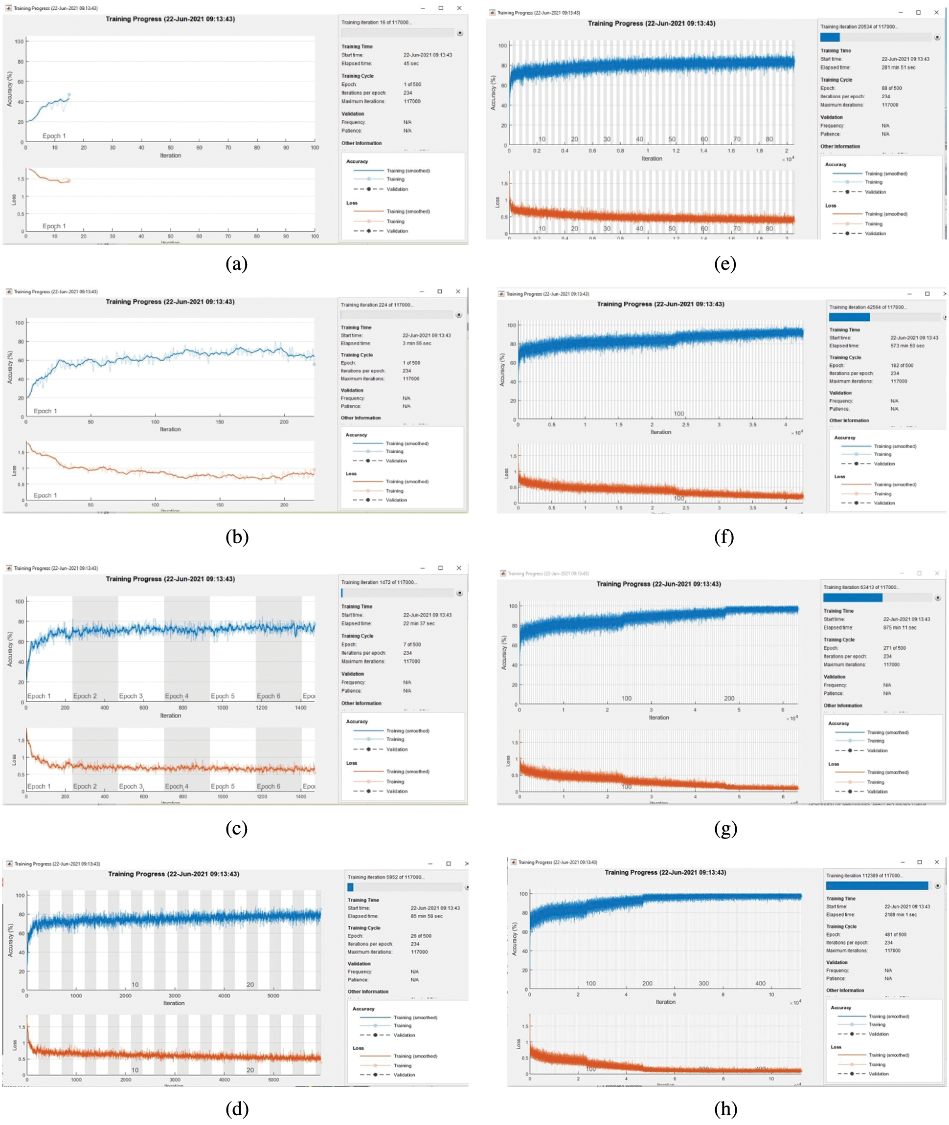
Figure 8: (a) Accuracy vs. iteration at 45 s (b) Accuracy vs. iteration at 3 min (c) Accuracy vs. iteration at 22 min (d) Accuracy vs. iteration at 85 min (e) Accuracy vs. iteration at 281 min (f) Accuracy vs. iteration at 573 min 59 (g) Accuracy vs. iteration at 875 min (h) Accuracy vs. iteration at 2900
A 64-bit operating system AMD A4-5000 APU with Radeon (TM) HD graphics with 1.50 GHz and 8:00 GB RAM is utilized in conjunction with MATLAB 2019a for modeling, processing, comparisons and visualizing the experimental numbers and findings through various deep learning algorithms such as Support Vector Machine (SVM), Neural Network (NN), K-Nearest Neighbor (KNN), Naive Bayes (NB), Ensemble (EN) and LSTM.
4.4.1 LSTM Performance for Various Input Features
The performance of the LSTM classifier is examined using a variety of methods, one of which is shown in Tab. 7. The 12 input features of the planned study are compared to various computations in this section. When compared to other features, the error rate of PM10 was determined to be lower.

4.4.2 LSTM Performance for Various Computations
Fig. 9 shows how the accuracy level of each feature is assessed. For each of the 12 input features, various other metrics like as error rate, sensitivity, specificity, accuracy, and F1score were determined individually. It was found that accuracy is high for PM10 and low for Xylene.
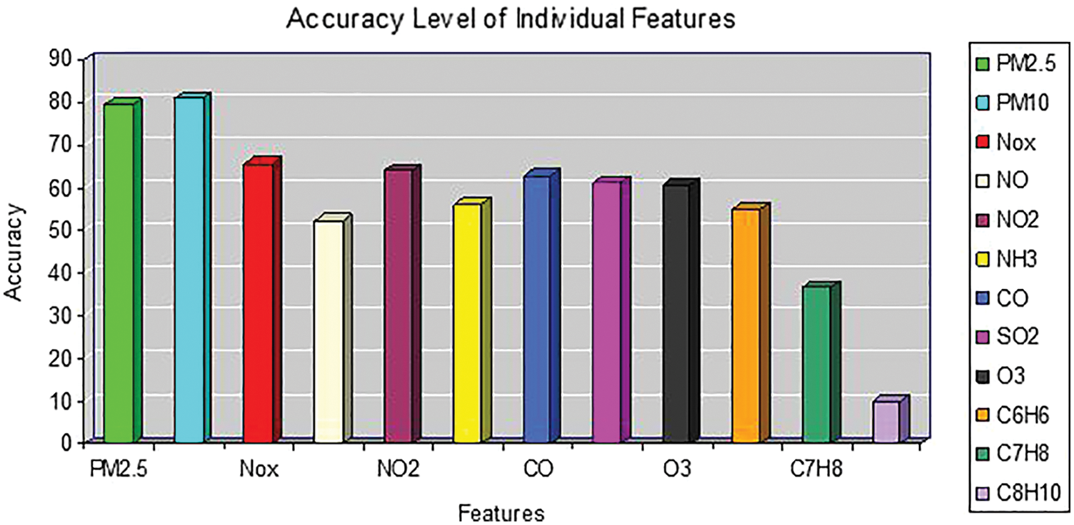
Figure 9: Accuracy level comparison of all input features
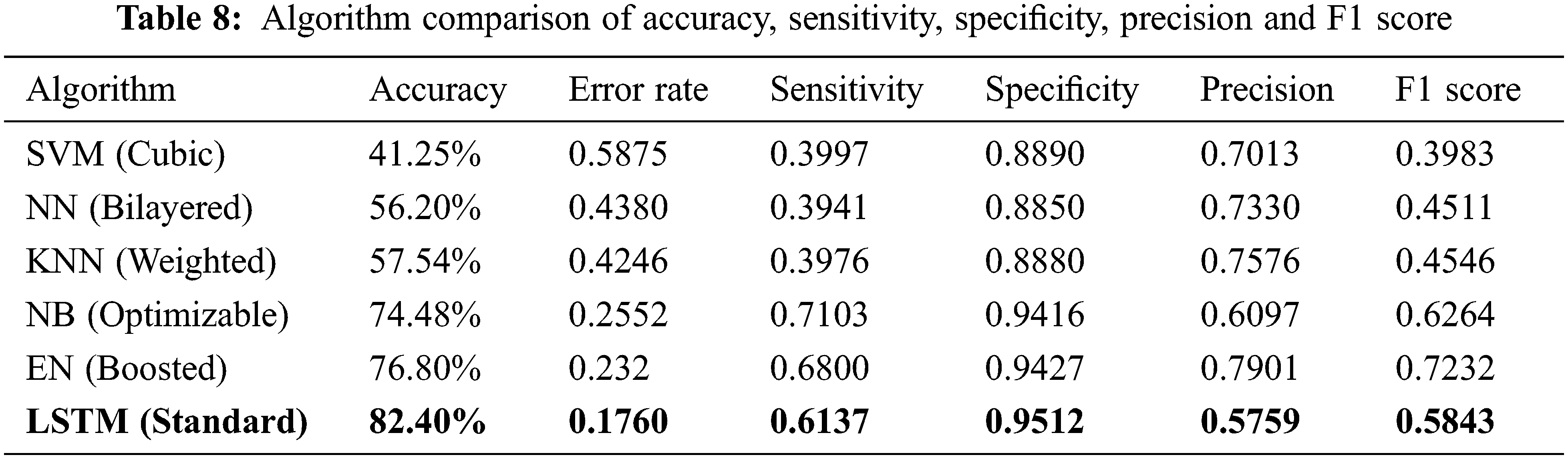
4.4.3 Algorithm Comparison with Proposed Work
Fig. 10 depicts the accuracy level of several approaches used, with the LSTM method proving to be the most accurate. Six different algorithms were taken for comparison for the same set of inputs.
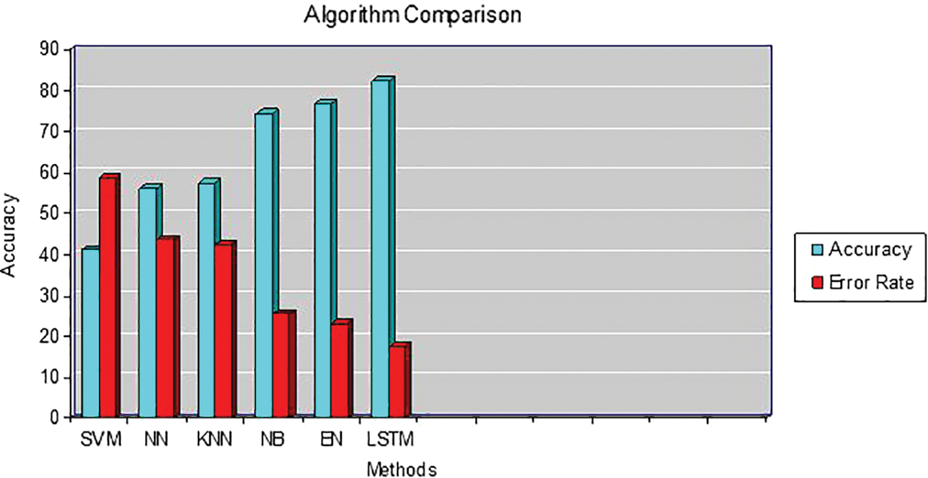
Figure 10: Accuracy level for various algorithms
As a result, various measures were examined using the LSTM approach, as shown in Tab. 8. The error rate found is minimum for the proposed LSTM method and subsequently accuracy is better compared to other methods.
4.5 Limitations of Study and Future Work
The study’s shortcoming was that the computation time was prolonged. The proposed study also has the disadvantage of not monitoring air pollutant concentrations in conjunction with other AQMS around or adjacent to it. Normally, both physical and chemical features of aerosols are used to predict air quality, however biological components and qualities are limited in this case. To increase the measurement level, future work can be expanded by including more air contaminants and additional data such as satellite images and industrial emissions into the atmosphere. To further understand the consequences of air pollution and human action, the article can be expanded by looking at specific states in relation to the current pandemic, as well as the situation before and after lockdown. Also, harmful air pollutants can be projected in advance for specific sites such as homes or roads, and the same can be combined with Internet of Things (IoT) and updated in real time in cloud computing for the benefit of people.
Based on historical air pollutant concentration, meteorological and time stamp data, this study provides an LSTM algorithm for predicting air pollutants in various sites. For predicting 12 major air contaminants, fine-grained air quality data is taken from active AQMS in 21 states across the country, India. Using the same dataset, six other models, including the proposed LSTM model, are evaluated, and the trials show that the suggested LSTM outperforms other techniques. By classifying air quality data and calculating dirty pixels using an LSTM classifier, the suggested work assists in obtaining specific information and permits precise knowledge of current pollutant levels in real environments of many sites. The classifier outputs the air pollutant level with higher compilation and efficiency than earlier approaches by comparing ground readings and data obtained from specific areas through private agencies, as well as suitable network training. The proposed approach delivers the best accuracy 82.4 percent of air pollution measurements for approximately 12 major air pollutants, according to the findings. This air quality measurement aids the environmental board in notifying the public and diverting traffic to low-polluting routes or areas, as well as taking appropriate measures such as tree planting, by anticipating air pollutants in advance.
Acknowledgement: The authors would like to thank Central Pollution Control Board of India (https://app.cpcbccr.com/AQIIndia/), for gathering information.
Funding Statement: The authors received no specific funding for this study.
Conflicts of Interest: The authors declare that they have no conflicts of interest to report regarding the present study.
1. A. P. K. Tai, L. J. Mickley and D. J. Jacob, “Correlations between fine Particulate Matter (PM2.5) and meteorological variables in the United States: Implications for the sensitivity of PM2.5 to climate change,” Atmospheric Environment, vol. 44, no. 32, pp. 3976–3984, 2010. [Google Scholar]
2. H. Zhang, S. Zhang, P. Wang, Y. Qin and H. Wang, “Forecasting of particulate matter time series using wavelet analysis and wavelet-ARMA/ARIMA model in Taiyuan, China,” Journal of the Air & Waste Management Association, vol. 67, no. 7, pp. 776–788, 2017. [Google Scholar]
3. C. H. M. Tong, S. H. L. Yim, D. Rothenberg, C. Wang, C. Y. Lin et al., “Assessing the impacts of seasonal and vertical atmospheric conditions on air quality over the Pearl River Delta region,” Atmospheric Environment, vol. 180, pp. 69–78, 2018. [Google Scholar]
4. W. Sun and J. Sun, “Daily PM2.5 concentration prediction based on principal component analysis and LSSVM optimized by cuckoo search algorithm,” Journal of Environmental Management, vol. 188, pp. 144–152, 2017. [Google Scholar]
5. G. Chen, S. Li, L. D. Knibbs, N. A. S. Hamm, W. Cao et al., “A machine learning method to estimate PM2.5 concentrations across China with remote sensing, meteorological and land use information,” Science of the Total Environment, vol. 636, pp. 52–60, 2018. [Google Scholar]
6. X. Hu, J. H. Belle, X. Meng, A. Wildani, L. Waller et al., “Estimating PM2.5 concentrations in the conterminous United States using the random forest approach,” Environmental Science & Technology, vol. 51, no. 12, pp. 6936–6944, 2017. [Google Scholar]
7. K. Huang, Q. Xiao, X. Meng, G. Geng, Y. Wang et al., “Predicting monthly high-resolution PM2.5 concentrations with random forest model in the North China Plain,” Environmental Pollution, vol. 242, pp. 675–683, 2018. [Google Scholar]
8. Y. Zhang and Z. Li, “Remote sensing of atmospheric fine Particulate Matter (PM2.5) mass concentration near the ground from satellite observation,” Remote Sensing of Environment, vol. 160, pp. 252–262, 2015. [Google Scholar]
9. B. T. Ong, K. Sugiura and K. Zettsu, “Dynamically pre-trained deep recurrent neural networks using environmental monitoring data for predicting PM2.5,” Neural Computing and Applications, vol. 27, no. 6, pp. 1553–1566, 2016. [Google Scholar]
10. Y. Qi, Q. Li, H. Karimian and D. Liu, “A hybrid model for spatiotemporal forecasting of PM2.5 based on graph convolutional neural network and long short-term memory,” Science of the Total Environment, vol. 664, pp. 1–10, 2019. [Google Scholar]
11. X. Li, L. Peng, X. Yao, S. Cui, Y. Hu et al., “Long short-term memory neural network for air pollutant concentration predictions: method development and evaluation,” Environmental Pollution, vol. 231, pp. 997–1004, 2017. [Google Scholar]
12. D. Qin, J. Yu, G. Zou, R. Yong, Q. Zhao et al., “A novel combined prediction scheme based on CNN and LSTM for urban PM2.5 concentration,” IEEE Access, vol. 7, pp. 20050–20059, 2019. [Google Scholar]
13. D. Seng, Q. Zhang, X. Zhang, G. Chen and X. Chen, “Spatiotemporal prediction of air quality based on LSTM neural network,” Alexandria Engineering Journal, vol. 60, no. 2, pp. 2021–2032, 2021. [Google Scholar]
14. C. Wen, S. Liu, X. Yao, L. Peng, X. Li et al., “A novel spatiotemporal convolutional long short-term neural network for air pollution prediction,” Science of the Total Environment, vol. 654, pp. 1091–1099, 2019. [Google Scholar]
15. J. Ma, Y. Ding, V. J. L. Gan, C. Lin and Z. Wan, “Spatiotemporal prediction of PM2.5 concentrations at different time granularities using IDW-BLSTM,” IEEE Access, vol. 7, pp. 107897–107907, 2019. [Google Scholar]
16. P. W. Soh, J. W. Chang and J. W. Huang, “Adaptive deep learning-based air quality prediction model using the most relevant spatial-temporal relations,” IEEE Access, vol. 6, pp. 38186–38199, 2018. [Google Scholar]
17. Y. S. Chang, H. T. Chiao, S. Abimannan, Y. P. Huang, Y. T. Tsai et al., “An LSTM-based aggregated model for air pollution forecasting,” Atmospheric Pollution Research, vol. 11, no. 8, pp. 1451–1463, 2020. [Google Scholar]
18. S. V. Belavadi, S. Rajagopal, R. Ranjani and R. Mohan, “Air quality forecasting using LSTM RNN and wireless sensor networks,” Procedia Computer Science, vol. 170, pp. 241–248, 2020. [Google Scholar]
19. Y. Han, J. C. Lam, V. O. Li and D. Reiner, “A Bayesian LSTM model to evaluate the effects of air pollution control regulations in Beijing, China,” Environmental Science and Policy, vol. 115, no. 11, pp. 26–34, 2021. [Google Scholar]
20. L. Zhang, P. Liu, L. Zhao, G. Wang, W. Zhang et al., “Air quality predictions with a semi-supervised bidirectional LSTM neural network,” Atmospheric Pollution Research, vol. 12, no. 1, pp. 328–339, 2021. [Google Scholar]
21. C. Olah, “Understanding LSTM Networks,” 2015. [Online]. Available: https://colah.github.io/posts/2015-08-Understanding-LSTMs/. [Google Scholar]
 | This work is licensed under a Creative Commons Attribution 4.0 International License, which permits unrestricted use, distribution, and reproduction in any medium, provided the original work is properly cited. |