DOI:10.32604/csse.2022.024303
| Computer Systems Science & Engineering DOI:10.32604/csse.2022.024303 | |
| Article |
Air Quality Predictions in Urban Areas Using Hybrid ARIMA and Metaheuristic LSTM
Department of Electronics and Instrumentation Engineering, SRM Institute of Science and Technology, Chennai, 603203, Tamilnadu, India
*Corresponding Author: S. Gunasekar. Email: gs9063@srmist.edu.in
Received: 12 October 2021; Accepted: 15 December 2021
Abstract: Due to the development of transportation, population growth and industrial activities, air quality has become a major issue in urban areas. Poor air quality leads to rising health issues in the human’s life in many ways especially respiratory infections, heart disease, asthma, stroke and lung cancer. The contaminated air comprises harmful ingredients such as sulfur dioxide (SO2), nitrogen dioxide (NO2), and particulate matter of PM10, PM2.5, and an Air Quality Index (AQI). These pollutant ingredients are very harmful to human’s health and also leads to death. So, it is necessary to develop a prediction model for air quality as regular on the basis of monthly or seasonaly. In this work, a new hybrid model for air quality prediction (AQP) is developed by using reed deer metaheuristic optimized Long Short Term Memory (LSTM) Deep Learning network. To overcome the drawback of the existing autoregressive integrated moving average model (ARIMA) model, the residual errors are processed by using an optimized LSTM network. The red deer optimization (RDO) is a new type of metaheuristic method which is motivated by the mating behaviour of Red Deer. The proposed model is better in terms of all prediction performance parameters when compared with other models.
Keywords: Air quality; prediction; ARIMA; RDO
The world is undergoing many new innovations related to smart engineering applications. These rapid growths of smart products, vehicles, machinery and the manufacturing industries are increased in the urban areas due to the overpopulations. The world’s population are increased drastically in recent days that may cause the scarcity of climate change, deforestation, natural resources and especially environmental pollution. In a recent survey, half of the world’s population is selected to live in the urban areas mostly. This survey may expect in future 2050 that 66% of people would live in the urban areas because of its convenience and flexibility. This kind of urbanization trend has happened in most of the developing and underdeveloped countries [1].
Due to the urbanization trends and its usages, the study proved that the air quality is not within the guidelines of the World Health Organization (WHO). The developed countries and the under-developed countries are undergoing these air quality issues. According to the report, nearly 100,000 populated cities of 98% from several countries do not contain healthy environmental air. In addition, there are many deaths are occur due to air pollution which is estimated so far as 3.3 million annual deaths worldwide [2].
Some of the pollutants that caused the air pollution and an unhealthy environment are sulfur dioxide (SO2), nitrogen dioxide (NO2), and particulate matter of PM10, PM2.5, and an Air Quality Index (AQI) [3]. These sorts of pollutant’s levels are estimated using the Tamil Nadu Pollution Control Board (TNPCB) which is measured and controlled the overall quality of air. These parameters are supported for the measurement of pollution that occurred in the atmospheric air but the accuracy of air quality is based on the Meteorological characteristics. So that there is a need to estimate location-based Meteorological characteristics parameters like temperature, humidity, wind speed and pressure respectively [4]. This Meteorological characteristic location is used to predict the complex airflow around the urban areas. The worst quality of air and occurrences of maximum pollutants may cause the oxygen demand and leads to heart diseases for human.
Many scholars have demonstrated are developed multiple predictions and survey to measure the pollutants and health issues of humans. These air quality predictions (AQP) are focused on human health especially for heart conditions to increase and also maximize good respirations for the people with asthma, children, the elder and for some emergency care people. Most of the scholars are used to predicting the timely series of Air quality based on the autoregressive integrated moving average model (ARIMA) technique that contains only a linear model. Though, the ARIMA predictions are not solvable yet, so that there is a need for some more advanced techniques with the optimal solutions for overcoming the environmental issues.
This paper is aimed to construct both the linear and non-linear model, the ARIMA is combined with the most powerful approaches of Long Short Term Memory (LSTM) based on Deep learning (DL) techniques. This hybridization of ARIMA and the LSTM model is used to attain both linear and nonlinear tendency respectively. The LSTM model is based on the Recurrent Neural Network (RNN) approach that is able to predict the sequence issues by learning order requirements. This method provides a better result about the AQP which is not so optimal in range. Therefore the LSTM is undergoing the process of optimization using the metaheuristics methods. Instead of presuming the result, the optimal solutions are to be carried out with an exact solution. so that the hyperparameter of LSTM is optimized by using metaheuristics methods of Red Deer optimization (RDO). The RDO is the recent popular metaheuristic approach that is motivated by the red deer’s behaviour in a breeding season. This RDO is used to overcome the issues of optimization and RSO operators are utilized some modified strategies to achieve the optimizer performances. The proposed model of LSTM hyperparameters is optimised using the RDO based on its biases and weights.
In this work, the three main methods are implemented to achieve an optimal prediction result namely the ARIMA model, LSTM model and the RDO model respectively. This method is partitioned into two sections which are used to forecast the non-linear and the linear result of AQP. The Linear results are provided using the ARIMA model and the non-linear part is carried out with the LSTM model. To obtain an optimal solution, the RDO is included to provide an exact fitness based on the weights and biases of LSTM parameters. Therefore, the proposed method is named a Hybrid ARIMA-LSTM-RDO (HALR) technique which has a good prediction in terms of prediction and error evaluations.
The rest of this work is explored as: the related work of existing literature is discussed in Section 2. Section 3 is explained the preliminaries about the ARIMA model and Section 4 is described the proposed methodology flow with detailed explanations. Section 5 showed the results and discussion of the proposed HALR technique and the work is concluded in Section 6. Finally, the references of this work are listed at the end.
In this section, the existing part of the literature that are derived numerous scholars with a mathematical model to achieve a high quality of forecasting.
In Yang et al. [5], the model based on ARIMA, empirical mode decomposition (EMD) and the support vector regression (SVR) are hybridized for predicting stock index. In the paper [6], a hybrid model of ARIMA and complex neuro-fuzzy are presented for predicting the financial time series by Li et al. The ARIMA is hybrid with the many ML techniques for the various prediction wherein the Khashei et al. [7], another hybrid of ARIMA and artificial neural networks (ANNs) are used for the prediction of financial data inspection. The Ordóñez et al. [8] have explored that the hybrid model with the machine learning of support vector machine (SVM) and the ARIMA for measuring the life of aircraft engines. The approach of ML-based SVM and the seasonal ARIMA (SARIMA) is discussed in Chen et al. [9] for forecasting the machinery productions in Taiwan. There was a prediction of time series based on the ambient O3 concentrations by using the model of ARIMA and singular spectrum analysis (SSA) in Kumar [10].
In many cases, deep learning (DL) based LSTM is applied for its accurate and efficient prediction in various fields. In Chen et al. [11], the LSTM method of sequential features is used to predict the China stock market’s exchange data. The paper of performance comparison between the ARIMA and LSTM based on the financial and economic data are explored in Siami Namini et al. [12]. In the [13], the Hybrid method of LSTM and ARIMA approach was estimated by Choi et al. that are used for the prediction of stock price correlation coefficient. Bukhari et al. [14] discussed a hybrid method of ARFIMA-LSTM based filters which is used for the prediction of abrupt stochastic variation. Song et al. [15] presented a Residual Network (ResNet) with LSTM for PM 10 and PM 2.5 ranges prediction. A spatial-temporal feature from sequential Aimage smartphones is estimated instead of PM 10 and PM 2.5 ranges at specific times and locations.
Gilik et al. [16] presented a hybrid of supervised models namely LSTM and convolution Neural Network (CNN) for AQP. This AQP is estimated by using sensor data among the cities. In another method Chang et al. [17], the Aggregated LSTM is established for the AQP that joined local station of air monitoring, neighbourhood stations of industrial 20 areas, and exterior pollution sources stations. A hybrid model of LSTM and optimization model of RDO is designed for short-term crop yield forecasting by author Mythili [18].
In this section, the preliminary of the proposed HALR method is described. The proposed methodology has a hybrid model of ARIMA and LSTM for the prediction of linear and non-linear models. This section carried a brief explanation of the ARIMA model and LSTM which is given in the following.
An ARIMA model is categorised into three types namely Autoregressive (AR), integration (I), and a moving average (MA) which is named as an ARIMA. This model is used in econometrics and statistics to estimate every time period events. It can be used for the prediction of observing the details from the past data and predicting the future behaviours. The three main parameters of ARIMA are autoregressive (p) difference order (d) and moving average order (q) respectively. But the ARIMA has only constraints of predicting a linear function of past data and random errors for the future valued variables. Thus the expression for the ARMA model is given in the following.
where
where L indicates the lag operation.
For the sequences of unstable values, the difference operator is required.
Therefore the ARIMA hyperparameter of (p, d, q) is expressed in the following.
For the issues based on the time series predictions, the ARIMA is the better model that can be possibly used widely for several applications. It is the most possible model for the linear functional form that can only have a linear inner correlation of residuals among the time series. In this ARIMA, the non-linear functions cannot be obtained for the time series so that the linear function is not only applicable for a complex issue.
For the purpose of obtaining a non-linear function, the LSTM model is presented to train and relate the residuals for the predictions. Therefore the residual of ARIMA is getting into an input to the LSTM, then the model of LSTM is used to perform train and predict accurate residuals for the AQP. Therefore the detailed model LSTM is discussed with its objective function below.
The LSTM is one of the widely used DL methods which is based on RNN that are efficient on prediction performance. There is an important hidden module presented in an LSTM known as the memory module. It has three main gates in the structure of RNN that is input gate, candidate gate, forget gate and Output gate respectively. The Input gate is used for reading the data from the dataset and the forget gate is used for the purpose of storing the data. Then the output gates are used for the writing purpose. These gates are identical to the valves which affect the neuronal information transmission by the valve’s opening and closing. This process is used to estimate the present neuron data and the number of neuron data is passed to the next of it.
The interior structure of the LSTM is shown in Fig. 1. From this structure, the forget gate output value is varied among the 0 and 1. The forget gate function defines that the previous cell state is not required and current states can be updated with the necessary information for prediction. The forget state (is expressed in the following.
where σ′ is the activation function, W′ represents the weight matrices and the b′ represents the bias,
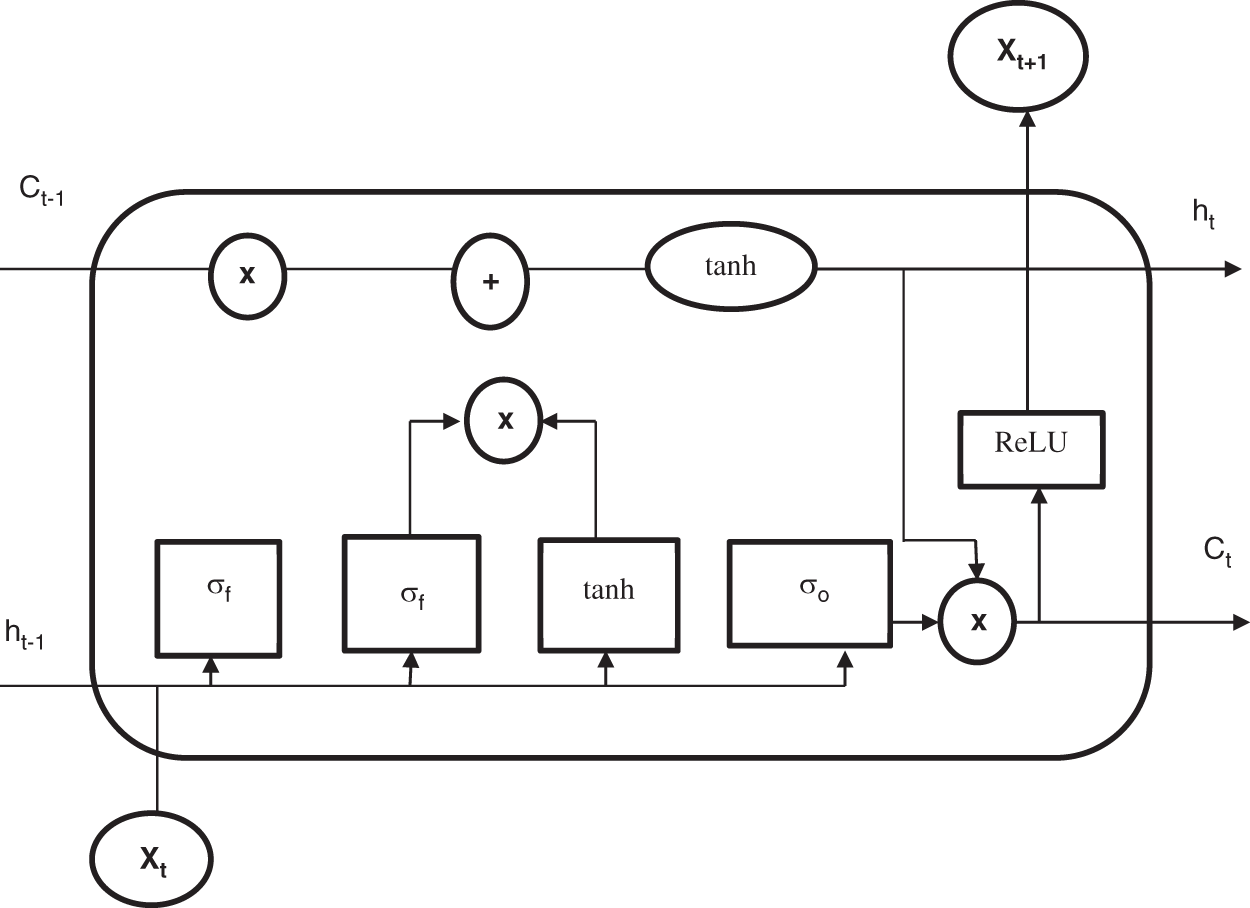
Figure 1: LSTM model
Next, the candidate Gate and Input Gate can be both activated to provide a next cell state Ct. This Ct is used to transfer to the new time step as a renewal cell state. The candidate Gate and Input Gate are provided with an activation function by sigmoid (σ′) and hyperbolic tangent function (tanh′) for estimating an output (
where the tanh lies between −1 and 1 and that are expressed as:
Therefore, the hybrid of both ARIMA and LSTM are combined for the linear and nonlinear prediction to obtain accurate results of AQP. Though these models are also do not provide an optimal result for a prediction. Thus this work proposes an LSTM hyperparameter be optimised by the metaheuristics RSO method.
This function is evaluated by the LSTM hyperparameter of weights and bias which is to be optimised by using the RSO. This function is used for minimizing error values and maximizing the higher prediction range in Air quality. During the training process, the RSO can be optimised for the weights and bias rates at every iteration. Therefore the Mean Square Errors (MSE′) can be expressed as:
where,
In the proposed methodology, the HALR method is presented which is the combination of the ARIMA model, LSTM model and the RDO model. The proposed HALR is designed to predict the AQP in urban areas. The overall workflow of the proposed HALR is given in Fig. 2. In this section, the proposed HALR explanation is provided for achieving the optimal best result in the AQP.
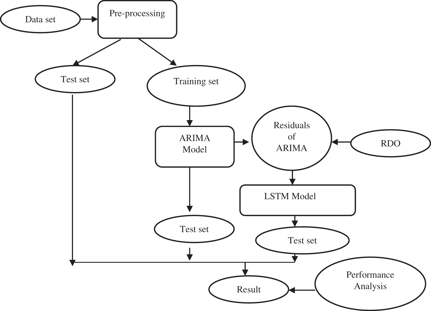
Figure 2: The overall workflow of proposed HALR
The urban area climatic data are collected from the website https://tnpcb.gov.in/air-quality.php which is the website of Tamil Nadu Pollution Control Board. This site is created to update the air quality due to the increment of industrial and commercial activities in the urban cities. So that, the ambient air quality is affected by industrial emissions due to the increment of vehicles. According to the act in 1981 named as Air Pollution Prevention and Control Act, the whole Tamil nadu state has been monitored to control an air pollution area.
The dataset included the climatic information of Chennai urban areas for the past 20 months which is from January 2020 to August 2021. This dataset obtained the air pollutants are SO2, NO2, PM10, PM2.5 and AQI to predict the air quality. This dataset is also included Meteorological characteristics such as temperature, apparent temperature, humidity, wind speed, wind bearing and pressure to obtain the flow of Air quality. These Meteorological characteristics are included to predict the complex airflow around the urban areas.
The pre-processing is categorised a data into two processes namely test data and train data. In this process, the more relevant data features are considered for a further process where the minimum relevant data features are ignored. This process carries 70%–80% of data for the training set and 20%–30% of data for the testing set. This data is given input to the ARIMA and LSTM model to predict both the linear and non-linear functions.
Initially, the ARIMA model is carried out for the prediction of the linear correlation part and then the residuals are achieved by deriving the original information with the suitable data. Therefore the residual of ARIMA is getting into an input to the LSTM, and then it is used to train and predict accurate residuals for the AQP. After that, the non-linear function is learned and derived by using the LSTM model. To obtain an optimal result in the prediction, the hyperparameter of LSTM can be optimised using a red Deer Optimisation (RDO) which is based on the metaheuristic method [18].
The red Deer optimization is a new type of metaheuristic method which is motivated by the mating behaviour of Red Deers. The abnormal mating characteristic of red deer has inspired the scholar Clutton-Brock who have studied it for more than twelve years and then is interested to construct an optimization strategy.
In this RSO, it is initialized randomly imitating the Red Deers. The presented quantities of optimal red deers are the male called as ‘stag’ where the remaining part of red deer belongs to female named as ‘hind’. The stag is used to roar to attract the hind deer. The hind is attracted by the roar capacity and its stamina of fighting ability. Then the stag is used to form a harem or group with a number of hinds. Thus the stag started to mate with the attracted hinds and some of the stags are also mated with another hind. This is the natural mating behaviour of red deer and the optimisation strategy is designed with this phenomenon.
In the proposed RSO methodology, the design of optimization mathematically without any constraints is used to solve issues that occurred in minimization. To obtain explorations and exploitations, the RDO contains three main parameters Alpha (α), Beta (β) and Gamma (γ). The parameters of α and β are used to handle diversifications. Then parameter of γ is used to balance intensifications. Where these three parameters of α, β and γ have lied between the intervals [0,1]. The diversifications are the process of measuring the roar and mating of stag and the hind that are presented randomly in the harem. Intensification is defined that to find the strongest stag known as commander, the fighting is conducted between the two stag or commander. Therefore the mating of a stag with a hind in its harem is presented in both diversification and intensification. The RSO can be attained with the several steps which are given below.
Step 1: Initialization
The RDO is also based on the population of stag and hind quantity that is generated randomly. The population quantity occurred in a solution space with dimensional Nvar optimization issues. Thus the best Red deer to the Nstag and rest in the Nhind for the purpose of mating.
The entire Red deer’s function values (FV) are
Step 2: Stag Roaring
This step shows the ability of stag by performing the highest roar that may also not be effective a few times. Since the red deer are an optimal result then the stag is determined and altered to the new place using below Expression
where, stago indicates the stag’s current place, stagn represents the new place of stag and
Step 3: Select γ% of best male deer stag as commander
Some of the males are more energetic, attractive or effective which can be measured by the number of commanders (MRDc) using an equation
where γ is the initial value between an interval (0, 1).
The quantity of stags (MRDstag) can be expressed by using an Eq. (8):
Step 4: The selection process is done through fights between the male commanders and stags:
Every commander of red deer fought with the stags at random to determine two new solutions. Finally, the selection of the best commander is derived with an objective function that is better than the previous result. So that the winner has high energy and the loser has low energy, then the objective function of Rn1 is represented as a new commander. These derivations are given in the following equations
where Rn1 and Rn2 represents the new results from the fighting, Com indicates the commander’s result and Stag indicates the stag’s result. The u1 and u2 are the random solutions of fight from uniform functional distribution in [0, 1].
Step 5: Harems formation
This harem is formed by a hind based on the commander energies with its effectiveness. Thus the hinds are categorised between the commanders to generate a harem which is expressed in the below equations
where the ecn represents the energy of nth commander and NVn indicates the commander normalized value.
The normalized energy of Male commanders is the number of hinds that are achieved by male commanders. Thus the hinds count in the harem
where the normalized value of entire commanders (
Step 6: The Mating of male Red Deer commander with α% hinds in its harem (
It is derived from an equation
Step 7: The male commander attacks another harem with β percent hinds for mating in another harem
Step 8: stag mating with the nearest hind:
In the breeding season, every stag is needed for mating with the closest hind where some of the hinds are favourite for a stag. Thus the j-distance space among the hind from the stag and its harem to another is expressed in the following equation.
where di represents the i-th distance range of hind or stag.
The Lower energy of stag is mated with the selected instead of a commander by using the equation
where, NR represents the new result and z represents an arbitrary uniform distribution function in [0,1].
Step 9: Select of Future generation:
The future generation selections are done by initializing commanders and stags that are retained. Next, it is selected by the production of child and hinds based on its fitness values. This process is not required any arithmetical formulation.
Step 10: Convergence:
Thus this process is involved with weights and biases in every iteration, and then an optimal result can be determined within a specific time period.
Therefore the proposed LSTM based RDO pseudocode is given in the following.
Pseudocode for proposed LSTM based RDO.
1. Set a hyperparameter of LSTM and MSE to initialize Red Deer.
2. Process the Roar of Red deer male
3. Update the place and position of every red deer using Eq. (11)
4. Selection of γ% to find a commander using an equations
5. Conduct fight among stag and commander using an equations
6. Update the position and place of stag and commander-13
7. Forming a Harem using an equations
8. Commander Mating with α% of hind in its harem using an Eq. (14)
9. Commander Mating with β% of hind in another harem using an Eq. (14)
10. Compute a stag mating with the closest hind using an Eq. (22)
11. Selection of future generation
12. Stop when the condition is satisfied with an optimal solution if not go to step 2
When the new generation fitness value attains a maximum value, then the process is ended with an updated weight and threshold values. The final updated optimal weight and threshold bias are applied to perform an LSTM. Then the result of AQP and an error evaluation is done with higher accuracy.
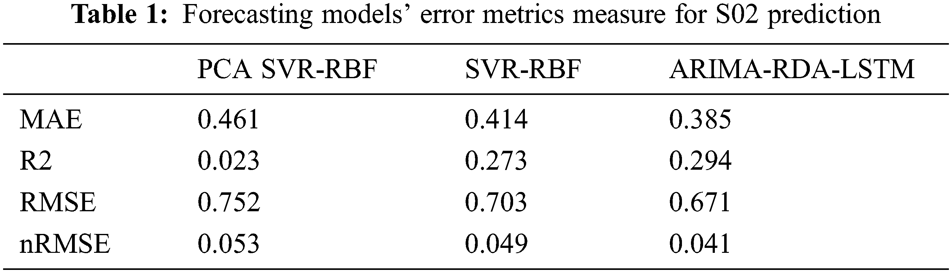
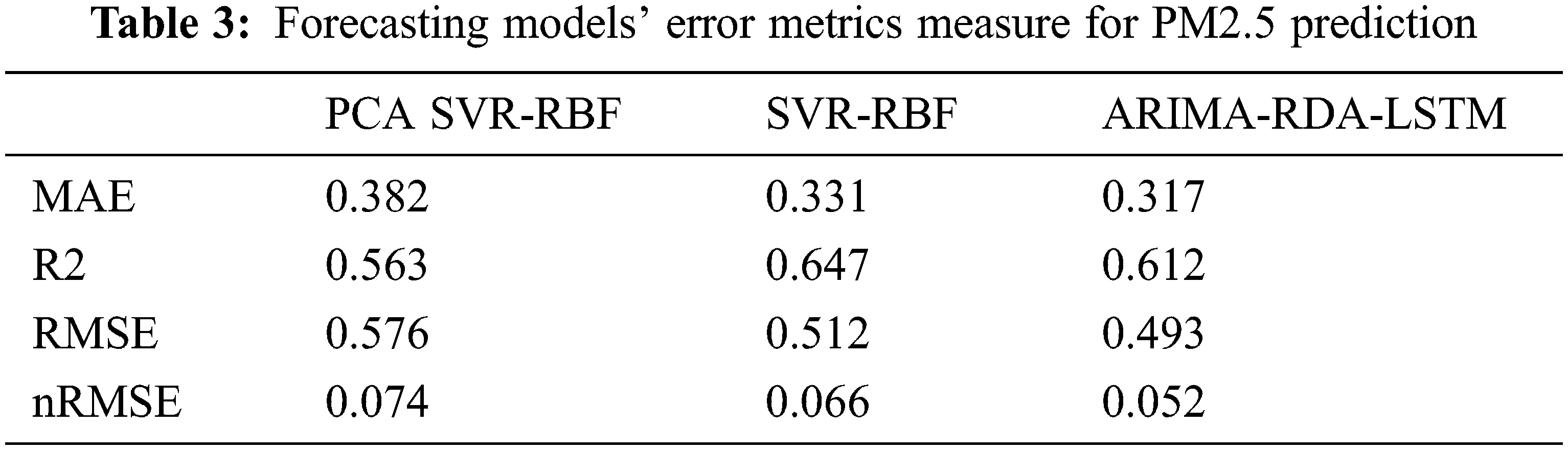
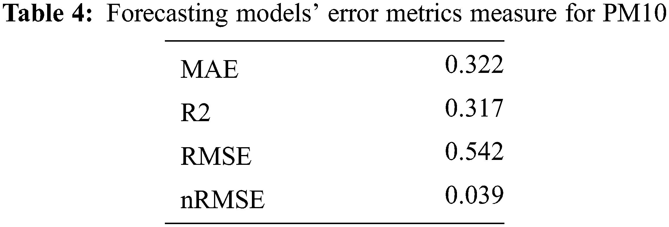
In this section, the experimental results are discussed the proposed HALR with the comparison of previous techniques SVM, KNN, hybrid ARIMA-LSTM and ARIMA model respectively. According to this proposed constrain, the dataset is carried out for training and testing in the ratio of 6:4 range. The proposed HALR is distinguished and verified to obtain its mean absolute error (MAE), the root mean squared error (RMSE), R2 score and the normalized RMSE (nRMSE). For a fair comparison, the proposed model compared against support vector regression (SVR)-radial basis function (RBF) and principal component analysis (PCA) based RBF prediction techniques. The obtained values of pollutants are given in Tabs. 1–5. From the tables observed that the proposed tuned model outperforms in terms of MAE, R2, RMSE and nRMSE for the forecasting of all pollutants. The precited values are nearly closer to the actual values shown in Figs. 3–7.
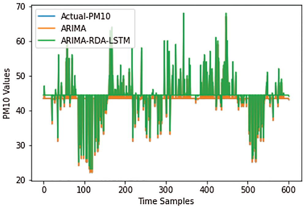
Figure 3: Observed and predicted values of PM10
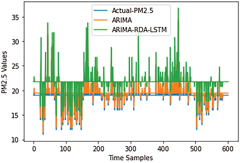
Figure 4: Observed and predicted values of PM2.5
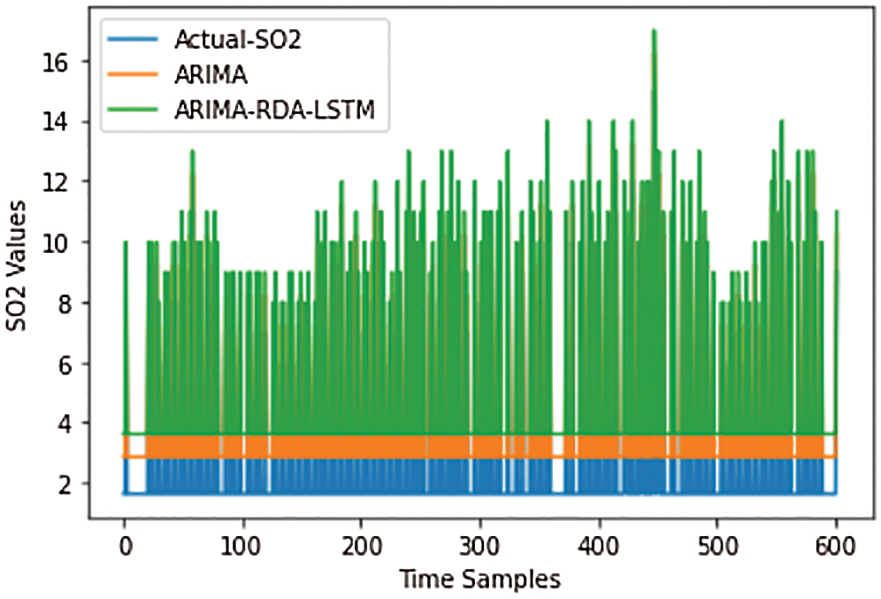
Figure 5: Observed and predicted values of SO2
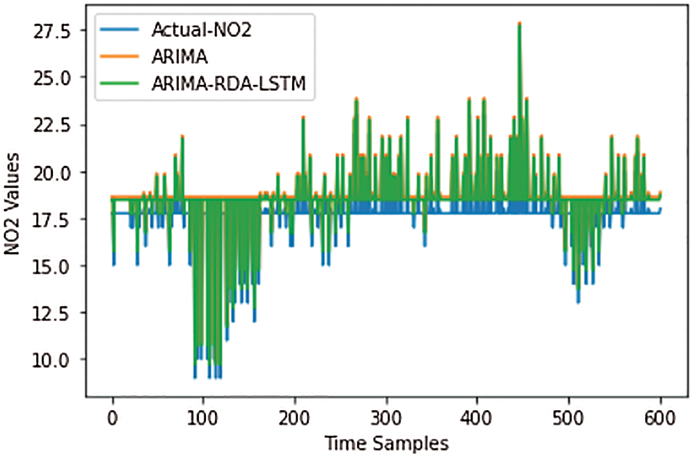
Figure 6: Observed and predicted values of N02
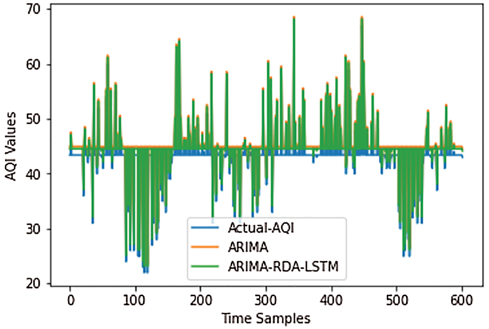
Figure 7: Observed and predicted values of AQI values

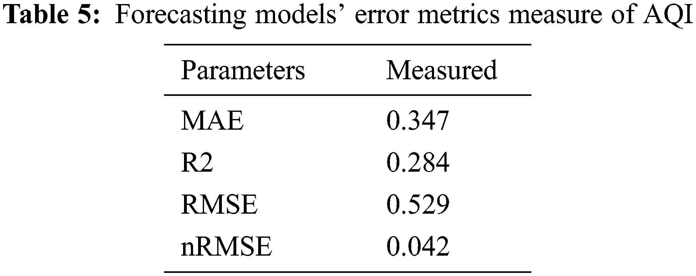
The forecasting errors of other models are higher than a proposed model for all pollutants predictions. Based on the observed values AQI values are calculated, the proposed model achieved MAE, R2, RMSE and nRMSE values of 0.374, 0.284, 0.529 and 0.042 respectively. To summarize, the proposed model is well suited for real-time air quality prediction compared to other models.
The proposed HALR is presented for the estimation of AQP which is done by the hybrid of ARIMA, LSTM and RDO methodology. In this proposed HALR, it can be obtained both the linear and non-linear functionalities perform complex issues. This proposed HALR is performed as an RDO based on weights and biases of the LSTM model for an exact prediction of Air quality. Therefore, the results are verified that the proposed HALR is significantly improved the quality of Air prediction. The HALR method is compared with the various models namely KNN, SVM, ARIMA and Hybrid ARIMA-LSTM respectively. The obtained result showed that the proposed HALR method is performed in all aspects with higher accuracy and prediction values. The error rate is evaluated with the parameters of MSE and RMSE that has been reduced in the proposed HALR than the prior models. Thus the result of prediction based on the parameters of accuracy, precision, recall and f-measure are performed well in the proposed HALR method. Compared to other models, the proposed model achieved MAE, R2, RMSE and nRMSE values of 0.374, 0.284, 0.529 and 0.042 respectively. So the proposed methodology is more robust and efficient than the previous networks that can be applied for a larger dataset in future. Future, the hybrid optimization algorithm will be introduced to solve the local minima problem of the optimization.
Funding Statement: The authors received no specific funding for this study.
Conflicts of Interest: The authors declare that they have no conflicts of interest to report regarding the present study.
1. H. Akimoto, “Global air quality and pollution,” Science, vol. 302, no. 5651, pp. 1716–1719, 2003. [Google Scholar]
2. B. R. Gurjar, A. S. Nagpure and P. Kumar, “Pollutant emissions from road vehicles in megacity Kolkat, India: Past and present trends,” Indian Journal of Air Pollution Control, vol. 10, no. 2, pp. 18–30, 2010. [Google Scholar]
3. M. Kampa and E. Castanas, “Human health effects of air pollution,” Environmental Pollution, vol. 151, no. 2, pp. 632–367, 2008. [Google Scholar]
4. K. Gu, J. Qiao and W. Lin, “Recurrent air quality predictor based on meteorology- and pollution-related factors,” IEEE Transactions on Industrial Informatics, vol. 14, no. 9, pp. 3946–3955, 2018. [Google Scholar]
5. H. L. Yang and H. -C. Lin, “An integrated model combined ARIMA, EMD with SVR for stock indices forecasting,” International Journal on Artificial Intelligence Tools, vol. 25, no. 2, pp. 165–172, 2016. [Google Scholar]
6. C. Li and T. Chiang, “Complex neurofuzzy ARIMA forecasting—A new approach using complex fuzzy sets,” IEEE Transactions on Fuzzy Systems, vol. 21, no. 3, pp. 567–584, 2013. [Google Scholar]
7. M. Khashei, M. Bijari and G. A. R. Ardali, “Improvement of autoregressive integrated moving average models using fuzzy logic and artificial neural networks (ANNs),” Neurocomputing, vol. 72, no. 4, pp. 956–967, 2009. [Google Scholar]
8. C. Ordóñez, F. S. Lasheras, J. Roca-Pardiñas and F. J. de Cos Juez, “A hybrid ARIMA–SVM model for the study of the remaining useful life of aircraft engines,” Journal of Computational and Applied Mathematics, vol. 346, no. 5, pp. 184–191, 2019. [Google Scholar]
9. K. Y. Chen and C. -H. Wang, “A hybrid SARIMA and support vector machines in forecasting the production values of the machinery industry in Taiwan,” Expert Systems with Applications, vol. 32, no. 1, pp. 254–264, 2007. [Google Scholar]
10. U. Kumar, “An integrated SSA-ARIMA approach to make multiple day ahead forecasts for the daily maximum ambient O3 concentration,” Aerosol and Air Quality Research, vol. 15, no. 1, pp. 208–219, 2014. [Google Scholar]
11. K. Chen, Y. Zhou and F. Dai, “A LSTM-based method for stock returns prediction: A case study of China stock market,” in 2015 IEEE Int. Conf. on Big Data (Big Data), Santa clara,United states, pp. 2823–3024, 2015. [Google Scholar]
12. S. Siami Namini and A. S. Namin, “Forecasting economics and financial time series: Arima vs. lstm,” Machine Learning, vol. 6, no. 5, pp. 1012–1019, 2018. [Google Scholar]
13. H. K. Choi, “Stock price correlation coefficient prediction with ARIMA-LSTM hybrid model,” Computational Engineering, Finance, and Science, vol. 3, no. 1, pp. 613–625, 2018. [Google Scholar]
14. A. H. Bukhari, M. A. Z. Raja and M. Sulaiman, “Fractional neuro-sequential ARFIMA-LSTM for financial market forecasting,” IEEE Access, vol. 8, no. 5, pp. 71326–71338, 2020. [Google Scholar]
15. S. Song, J. C. K. Lam and Y. Han, “ResNet-LSTM for real-time PM2.5 and PM10 estimation using sequential smartphone images,” IEEE Access, vol. 8, no. 5, pp. 220069–220082, 2020. [Google Scholar]
16. A. Gilik, A. S. Ogrenci and A. Ozmen, “Air quality prediction using CNN+LSTM-based hybrid deep learning architecture,” Environ. Sci. Pollut. Res., vol. 5, no. 7, pp. 115–123, 2021. [Google Scholar]
17. Y. S. Chang, H. T. Chiao and S. Abimannan, “An LSTM-based aggregated model for air pollution forecasting,” Atmospheric Pollution Research, vol. 11, no. 8, pp. 1451–1463, 2020. [Google Scholar]
18. K. Mythili, “A swarm based bi-directional LSTM-enhanced elman recurrent neural network algorithm for better crop yield in precision agriculture,” Turkish Journal of Computer and Mathematics Education (TURCOMAT), vol. 12, no. 10, pp. 7497–7510, 2020. [Google Scholar]
 | This work is licensed under a Creative Commons Attribution 4.0 International License, which permits unrestricted use, distribution, and reproduction in any medium, provided the original work is properly cited. |