DOI:10.32604/csse.2022.025029
| Computer Systems Science & Engineering DOI:10.32604/csse.2022.025029 | |
| Article |
Deep Convolutional Neural Network Based Churn Prediction for Telecommunication Industry
1Department of Computer Science, College of Computer, Qassim University, Buraydah, Saudi Arabia
2Department of Computing, School of Electrical Engineering and Computer Science, National University of Sciences and Technology (NUST), Islamabad, Pakistan
*Corresponding Author: Ali Mustafa Qamar. Email: al.khan@qu.edu.sa
Received: 08 November 2021; Accepted: 10 December 2021
Abstract: Currently, mobile communication is one of the widely used means of communication. Nevertheless, it is quite challenging for a telecommunication company to attract new customers. The recent concept of mobile number portability has also aggravated the problem of customer churn. Companies need to identify beforehand the customers, who could potentially churn out to the competitors. In the telecommunication industry, such identification could be done based on call detail records. This research presents an extensive experimental study based on various deep learning models, such as the 1D convolutional neural network (CNN) model along with the recurrent neural network (RNN) and deep neural network (DNN) for churn prediction. We use the mobile telephony churn prediction dataset obtained from customers-dna.com, containing the data for around 100,000 individuals, out of which 86,000 are non-churners, whereas 14,000 are churned customers. The imbalanced data are handled using undersampling and oversampling. The accuracy for CNN, RNN, and DNN is 91%, 93%, and 96%, respectively. Furthermore, DNN got 99% for ROC.
Keywords: Deep learning; machine learning; churn prediction; convolutional neural network; recurrent neural network
As the service industry becomes increasingly competitive, service-oriented enterprises must predict customer churn: the tendency of existing customers to leave the service provider, typically defined by the amount of time elapsed since they are engaged with the service. It costs much more—about six times more to acquire new customers than to retain existing ones [1] because the churn entails both lost revenue from the churned customers and marketing costs to acquire replacement customers. Besides, long-term customers tend to yield higher profits than new customers, and it typically is more complicated to reach new customers. For all of these reasons, every business should strive to reduce the churn.
The ability to predict customer churn is valuable because it enables enterprises to take active steps to discourage churn behavior and retain current customers [2]. Big data is increasingly captured in various domains, including finance, weather, business, and even healthcare; the challenge now is not how to obtain data but how to obtain useful information from the data. Central to this conversation are machine learning (ML) and statistical algorithms, which can mine vast datasets for patterns and extrapolate consequences without any actual knowledge of the domain [3].
Within the ML research community, various representation learning procedures apply to multiple levels of representation. However, recently, deep learning (DL) is emerging as a practical approach for discovering explanatory factors or features within various levels of particularly complex representations. The features at higher levels represent increasingly abstract aspects of the data [4]. This research applies DL techniques to a telecommunication dataset in order to predict customer churn. In contrast, customer churn analysis can be used to make business decisions and optimize various services. The DL model could also be applied to multiple domains.
The rest of the paper is organized as follows: the state-of-the-art is discussed in Section 2, followed by the dataset details in Section 3. The proposed methodology is presented in Section 4. Section 5 presents the experimental setup along with the results. The article is concluded in Section 6, along with giving some future directions.
Customer churn prediction is a significant affair in Customer Relationship Management (CRM). Nowadays, rapid lifestyle transformations have a severe effect on CRM, and customers can quickly shift between competitors. Thus, industries are moving their attention from gaining new customers to retaining their existing customer base. Consequently, there are some outstanding successes offered by such ML and DL techniques to the challenging problem in churn prediction, as will be discussed later. Prashanth et al. [5] use logistic regression, Random Forest, and DL architecture, including deep neural network (DNN), deep belief network (DBN), and recurrent neural network (RNN) for churn prediction in the telecom industry. Random Forest offered high performance in terms of accuracy, the Area under the ROC curve (AUC), and Specificity. However, RNN was able to show remarkable performance in terms of Sensitivity. Umayaparvathi and Iyakutti [6] proposed three deep architecture and built the corresponding churn prediction model using two telecom datasets. The three deep architecture are Feed-forward Neural Network (FNN), Convolutional Neural Network (CNN), and classification using ML vs. DL implementation using Python.
The experimental results show that DL-based models perform as valuable as traditional classification models while considering accuracy as the performance metric. According to the study by Castanedo et al. [7], the implementation of a multi-layer feed-forward architecture was significant enough to predict the churn. The used dataset contains Call Detail Records (CDR) and balance replenishment records, which show if the customer is active or has churned. The employed optimization technique was Stochastic Gradient Descent (SGD), and they apply dropout as well. For performance metrics only, AUC has been used to analyze the results. As future work, they suggested the use of deep belief networks.
Another related method was proposed by Karanovic et al. [8]. In this study, the researchers investigate the applicability of CNN on imbalanced data for churn prediction. They obtained an accuracy of 98% on a dataset from a telecommunication company named Orange. The optimization of the CNN hyperparameters was carried through grid search.
Furthermore, Rectified Linear Units (ReLU) was used as an activation function, and Adam was used as an optimization algorithm. This study shows that CNN achieves better accuracy than other ML algorithms. A recent review of the literature on this topic is performed by Agrawal [9]. The applied model is developed using feed-forward neural networks. A specific dropout layer has been added with a value of 0.1. The multi-layered ANN model results in an accuracy of 80.03%. The best results were obtained using Adam optimizer.
From the aforementioned discussion, although ML-based models are gaining traction with churn prediction and have the potential to deal with a considerable amount of data, DL models have not attained the full attention of researchers in this field [10,11]. In DL, only some papers have studied the problem of churn prediction in the telecommunication area. As seen from studies, predictive churn techniques can be broadly grouped into ANN and CNN techniques. To the best of our knowledge, no research has been done on the same dataset as considered in this study with a DL model. The dataset is used only in one study with ML using accuracy as performance metrics. Although ‘Accuracy’ is a good metric of performance, assessing performance just based on ‘Accuracy’ is insufficient because accuracy is more predictable and will be the same on small datasets. Other performance indicators, such as Precision, Recall, F-score, and AUC curve, should be considered in addition to Accuracy [12]. This study ensures that a variety of performance metrics were utilized to assess the outcome. In most cases, dropout and Adam are used in DL models for churn prediction. This technique will be used in this study since it has shown to be notably successful on other churn prediction tasks.
The data was obtained from a Telecom operator [13] with approximately 100,000 customers (active or churn) in a CSV file containing three months of customer history. The data set contained 48 attributes, including traffic type (outgoing/incoming for voice, SMS, and data), destination (on-net, off-net), loyalty, and traffic behavior. The status of the customer, which can be active or churn, is the class attribute. Tab. 1 provides details about some of the dataset attributes.

The first two months were used for training and validation, while the third one was kept for testing. The data is split into training and validation/testing sets with a 67/33 split.
Classification models usually perform best when the class distribution is almost equal. The dataset is imbalanced if the class is not in a 50/50 or 60/40 distribution. Our dataset is an imbalanced one. The proposed technique is a combination of under-sampling and oversampling for dataset balancing to improve the classification results. The process was performed using the WEKA toolkit. In the under-sampling approach, some instances are deleted from the majority class (Active class), so that the number of instances in the majority class becomes close to those in the minority class. For this study, the Resample method is employed for under-sampling. This reduction is made randomly and is therefore known as random under-sampling. The oversampling process we used is called Synthetic Minority Oversampling Technique (SMOTE). In simple words, it looks at the feature space for the minority class data points, and considers its K nearest neighbors. After applying Resample and SMOTE on the dataset, we achieved a balanced dataset. As shown in Fig. 1, the churn class presents 40.38% of the total instances, while the active class presents 59.62% of the training set. Furthermore, in the testing set, the churn class contains 41.62% of the total instances, while the active class presents 58.37%.
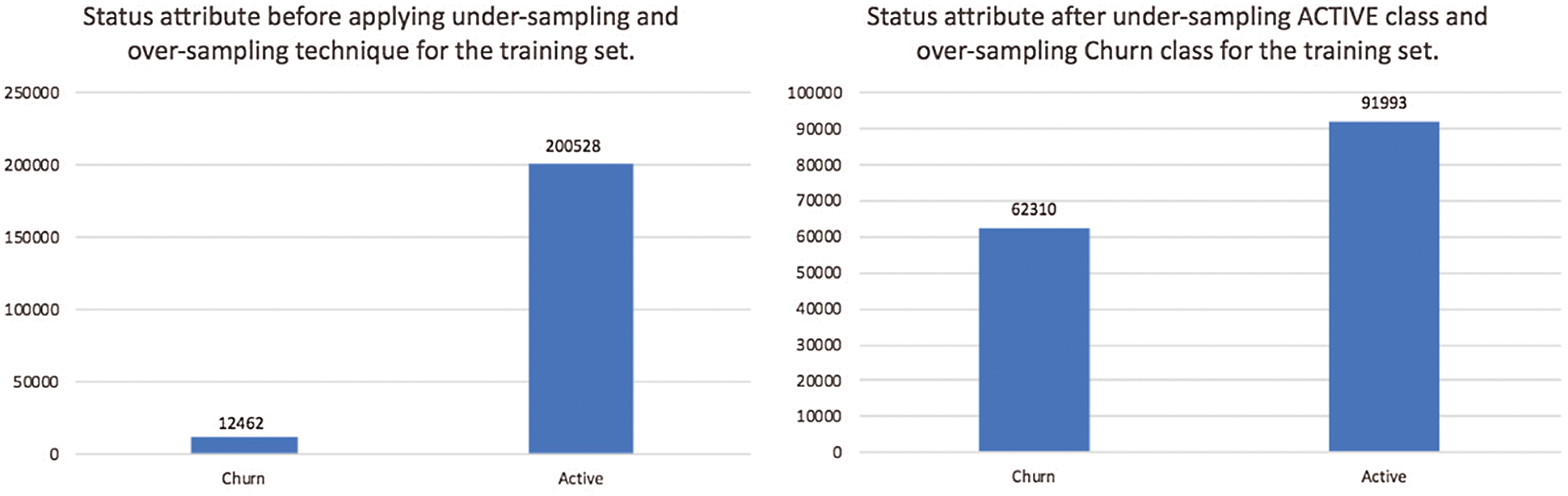
Figure 1: Histogram for the active and churn customers before and after under-sampling the active class and over-sampling the churn class for the training set
In this study, we provide a set of DL models for predicting customers who intend to churn from the company to improve churn prediction management. We built various models, which could be employed in any telecom industry to handle churn management in a better way. In particular, we want to prove that these techniques are sufficiently effective in boosting a telecommunication company’s retention power. We now discuss the experimental setup and the baseline methods that will be applied to certify the proposed approach’s efficiency.
The proposed churn prediction framework is presented in Fig. 2. The input data consists of the CDR. The data is passed to the data preprocessing stage. Here, the class imbalance problem is handled along with the normalization of the data (if required). Next, three proposed DL architecture are employed to achieve the desired goals of this research.
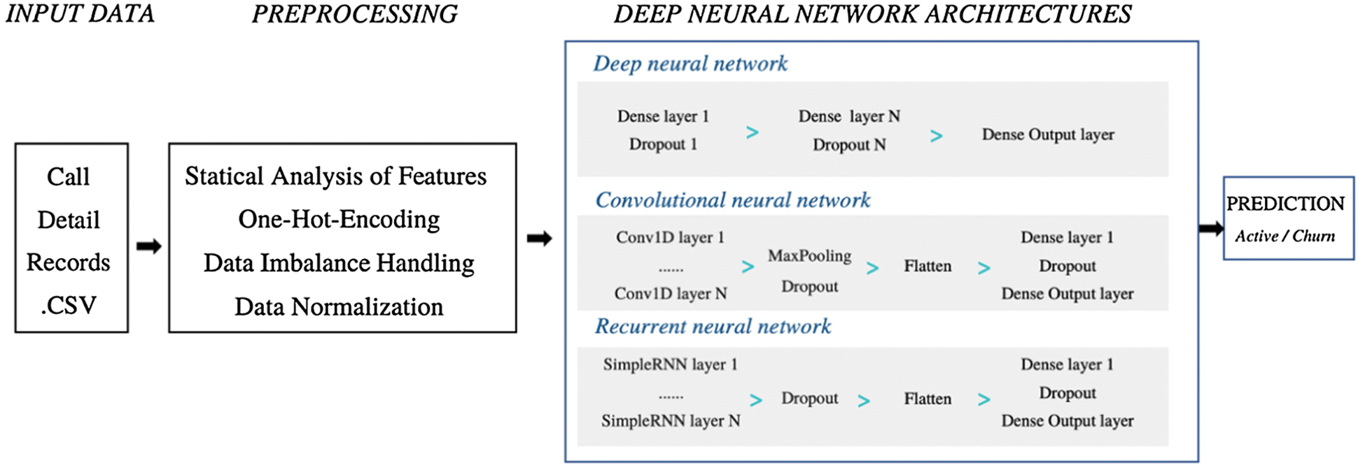
Figure 2: Proposed churn prediction framework
The essential tool to develop deep neural networks in Python is the Keras API, together with the TensorFlow in the backend. We implemented the entire model in the PyCharm environment. Furthermore, TensorFlow 1.11 was installed on a computer with OS X 10.10.5, a desktop with 8 GB RAM, and an Intel Core i5 Processor with 2.7 GHz. Our models run on the local CPU.
Here, we present the proposed DL architecture for the churn prediction task. The probability of the churn is predicted by introducing the users’ three month’s data into the model. This research presents three DL models, based on DNN, CNN, and RNN architecture. The proposed models are configured based on different hyperparameter tuning experiments. Hyperparameters are the variables that determine how the network is trained. During training and testing phases, multiple activation function settings were tried. The activation functions are extremely important since they learn the abstract features through non-linear transformations [14]. The configuration was selected based on the comparison of the performance of three activation functions which are Tanh, ReLU, and Sigmoid. Furthermore, four alternative training algorithms are used to boost the performance of networks [15]. The algorithms that were used were Adam [16], Nadam [17], SGD [18], and RMSprop [19]. The experiments show that Adam gives the highest results. Consequently, it is used for configuration.
4.2.1 Deep Neural Network Setup and Training
The initial values of the hyperparameters were carefully chosen according to the validation set results for different models. The first model is a deep neural network, founded on a multi-layer feed-forward network. According to Prashanth et al. [5], ANN can be used to accomplish the DL tasks while using more than two hidden layers. We initialized our model in Keras using a sequential model, which can be considered as a linear stack of neural layers and mainly involves dense layers. A dense layer is a fully connected (FC) layer. The model necessitates the data to the first layer with a definite shape. This input shape is determined by the number of initial parameters that have been extracted from the preprocessing stage (specifies the number of rows and columns in the input).
We used three hidden layers where each layer has 43 neurons. The number of hidden neurons was selected based on the rule-of-thumb method presented in Karsoliya’s study [20]. ReLU function performs the computation of activation for the dense layer. A dropout rate of 0.6 was used between each FC layer to avoid over-fitting. A sigmoid activation function was used following the single node’s output layer since our target class is either churn or active.
We compiled the model using the binary cross-entropy loss function and use the efficient Adam with a learning rate of 0.01. The number of epochs and the number of training iterations over the dataset were determined by early stopping on the validation set. The patience was set as 22, meaning that if the model does not improve after 22 epochs in a row, it will be stopped. The model’s performance was evaluated at the end of each training epoch on the test dataset with the default batch size. Tab. 2 displays the hyperparameters setting for the model.

Therefore, one of the goals of this study is to study if the overall performance of the presented network can be improved further at enhancing the model results. For that, another model has been implemented next.
4.2.2 Convolutional Neural Networks Setup and Training
We propose a one-dimensional CNN model for churn prediction. We used Keras conv1d function for developing the computation of convolution. In 1D CNN, the kernel moves in one direction. The 1D Conv model consists of two convolutional layers, having 32 filters (batch size) of kernel size 1. ReLU is employed as the activation function for the convolutional and FC layers.
Furthermore, the convolutional layer’s feature maps are the input of the pooling layer and are pooled to reduce the feature dimensions. MaxPooling (with a pool size of one) is used. Moreover, flatten and dropout (having a rate of 0.2) are applied between each FC layer to reduce overfitting. After using several convolutional and pooling layers, the last layer’s output becomes the input of an FC layer, which ultimately helps in classifying. Since we want to perform binary classification, the output of the FC layer is calculated by the sigmoid activation function. The structure of the 1D CNN model is presented in Fig. 3. The model is composed of an input layer defined by the dimension of the dataset, two convolutional (Conv) layers, two pooling layers, and an FC and output layer.
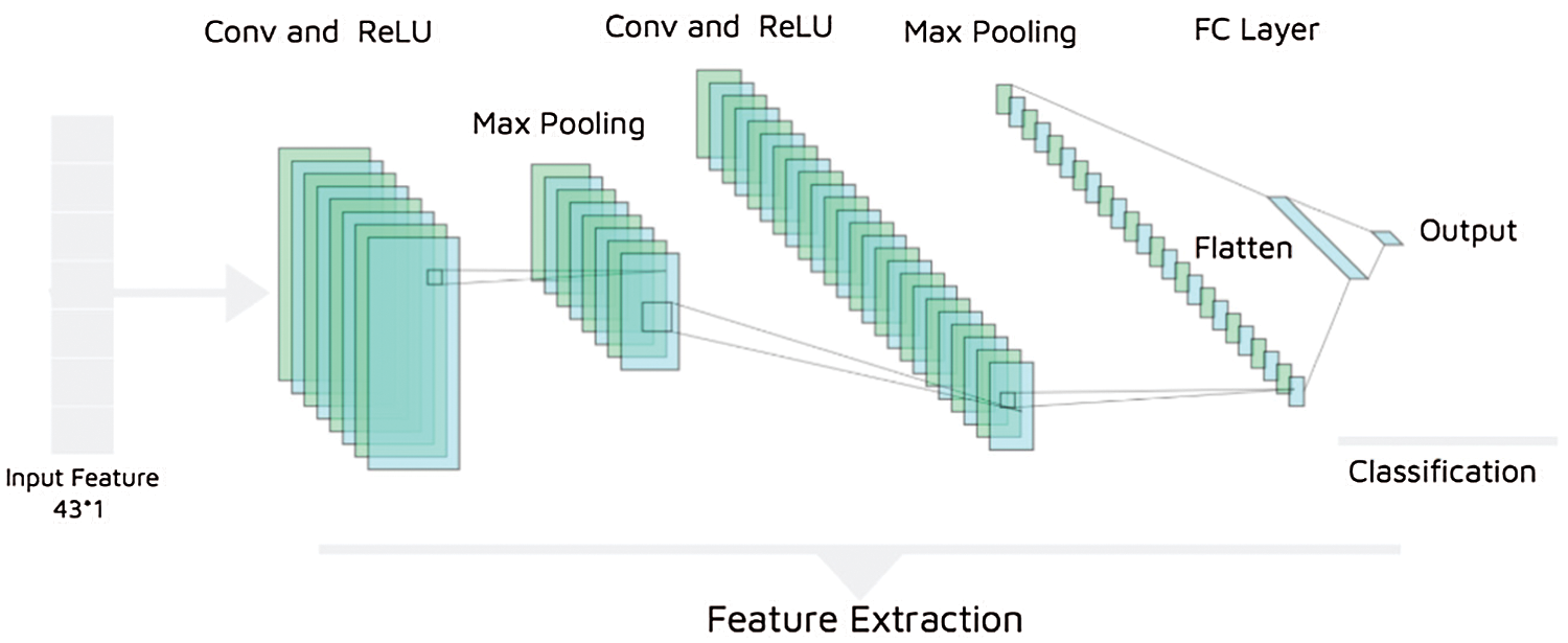
Figure 3: The architecture of the 1D CNN model
Adam is used for adapting the learning rate. The number of epochs was determined by early stopping, as was the case in the DNN model. After selecting the optimal values of different parameters, a predictive model was trained and evaluated using the first two months from the CDRs. The values of hyper-parameters for the CNN model are described in Tab. 3. The learning rate is smaller than that of DNN. However, the total number of parameters is much more than DNN.

4.2.3 Recurrent Neural Networks Setup and Training
According to a study by Prashanth et al. [5], RNN shows excellent results in many areas. Among the applied DL techniques, RNN performed better than DBN and DNN. Therefore, we employ an RNN architecture, except that we do not use Long Short-Term Memory (LSTM). Instead, we apply SimpleRNN, a fully-connected RNN, where the output is to be fed back to the input. An improvement in the results was observed while increasing the number of SimpleRNN layers. The RNN model is the same as that of an MLP with a hidden layer. However, the activations arrive at the hidden layer from the current external input as well as the hidden layer activations one step back in time. Compiling and fitting the model is the same as the CNN model. The model consisted of three stacked SimpleRNN layers with dropout to avoid over-fitting. The first, second, and third layers have 128, 64, and 32 units, respectively, followed by an FC layer.
We consider five baseline classifiers to compare the telecom industry data, mainly, Support Vector Machines (SVM), decision trees (J48), Naïve Bayes, logistic regression, and MLP. The reason for choosing these classifiers is that they are the most frequently used estimation techniques in churn prediction. The classification process for the underlying ML algorithms is performed using the WEKA toolkit.
Here, we introduce the performance metrics and the analysis of the experimental results to test the churn prediction models’ performance. Furthermore, a comparison of the proposed models with baseline methods and previous studies is also presented. Finally, we run different experiments to ascertain the performance of the hyperparameters.
Evaluating the performance of a model is the primary task in effective churn prediction. There are numerous performance metrics to compare various classifiers’ effectiveness for churn prediction. The metrics’ description is defined next:
Confusion matrix: It is essentially a table showing correct predictions and types of incorrect predictions that show the number of true positives (TP), true negatives (TN), false positives (FP), and false negatives (FN).
Accuracy: It is defined as the ratio of all correct decisions to the total number of decisions. It is presented in Eq. (1).
Precision: The number of true positives divided by all positive predictions, as shown in Eq. (2).
Recall (Sensitivity, True Positive Rate – TPR): The number of true positives divided by the number of positive values in the test data, as obtained in Eq. (3).
F1-score: The weighted average of precision and recall, as shown in Eq. (4). It is also defined as the harmonic mean of precision and recall.
Specificity (true negative rate): It corresponds to the number of churned cases identified correctly divided by the total number of negatives.
AUC curve: considers all thresholds on the predicted probabilities. The closer the AUC of a classifier is to 1, the higher is the accuracy of the method.
Receiver Operating Characteristic (ROC): It can help in deciding the best threshold value. The ROC graph plots TPR against FP rates.
Cohen’s Kappa: It calculates the percentage of data values in the principal diagonal of the confusion matrix and fine-tunes these values for the amount of agreement that could be anticipated because of chance alone.
Once the model has been built and compiled, the next step is to fit the dataset’s proposed models. Three months of data have been provided. The first two months’ data were used for training (123,442 samples) and validation (30,861 samples) with an 80:20 split, while the third month was used for testing, which contains 74,847 samples.
The model was trained with 22 epochs, using the early stopping regularization technique, which stops at epoch 21. The number of epochs was selected based on running the model without early stopping with 30 epochs. However, there is no improvement in the results. The accuracy for training and validation sets against the epochs is shown in Fig. 4. Similarly, Fig. 5 presents the training and validation loss curve.

Figure 4: The graph on the left shows the training accuracy curve. Similarly, the one on the right shows the validation accuracy for the most accurate DNN model against the number of epochs. The best training accuracy is 0.9918, and the validation accuracy is 0.9956

Figure 5: Training and validation loss curves for the most accurate DNN, where the training and validation losses are 0.0486 and 0.0138, respectively
From Fig. 4 and Fig. 5, one can observe a significant improvement in the accuracy and reduction in loss after the 8th epoch. The accuracy saturated around the 20th epoch, where its value reached 0.992. Tab. 4 shows the confusion matrix of the model.

On the left side of Fig. 6, the orange line shows the Precision-Recall curve in the testing phase —the precision results on the y-axis and the recall results on the x-axis. The Area under the curve is the Area under the Precision-Recall curve (AUPRC). Similarly, the plot for the Area under the ROC curve (AUROC) is shown at the right side of Fig. 6, which shows the amount of TP (recall) and FP rate for the DNN.

Figure 6: On the left is the Precision-Recall curve for the test set with DNN. On the right is the ROC curve for the test set with DNN
5.2.2 Convolutional Neural Networks
In the case of CNN, we train the model using early stopping regularization techniques based on the validation loss, which stops at epoch 14. The prediction training accuracy is enhanced by employing this approach, evident from the graph in Fig. 7. Fig. 8 presents the training and validation loss curves.

Figure 7: Training and validation accuracy curves for the most accurate CNN, where the best training and validation accuracy is 0.9994 and 0.9992, respectively

Figure 8: Training and validation loss curves for the most accurate CNN where the minimum training and validation loss are 0.0020 and 0.0019, respectively
Tab. 5 shows the confusion matrix for the 1D CNN model. The true positives and the true negatives were the values that the model predicted correctly (Active customers predicted and vice versa with churners).

Furthermore, the orange line on the left of Fig. 9 shows the Precision-Recall curve in the testing phase. On the right of Fig. 9, we show the amount of true positive (recall) and false-positive rates for 1D CNN.

Figure 9: On the left is the Precision-Recall curve for the test set for 1D CNN. On the right is the ROC curve for the test set for 1D CNN
5.2.3 Recurrent Neural Networks
While training the model using an early stopping regularization technique based on the validation loss, the model stops at epoch 13. The training and validation sets’ accuracy for various epochs is shown in Fig. 10.

Figure 10: Training and validation accuracy curves for RNN, where the best training and validation accuracy is 0.9994 and 0.9995, respectively
Tab. 6 shows the confusion matrix for the model. The confusion matrix is generated from the testing of the Simple RNN model.

On the left of Fig. 11, the orange line shows the Precision-Recall curve in the testing phase. Similarly, the plot for the ROC curve is provided in the right of Fig. 11, which shows the amount of true-positive (recall) and false-positive rates for the Simple RNN performance.

Figure 11: On the left side, the Precision-Recall curve for the test is shown. On the right, the ROC curve corresponding to the test set is shown
The results of the three proposed models in terms of accuracy, recall, Precision, Specificity, F1-score, ROC AUC, Precision-Recall Curve (PRC) AUC, and Cohen’s kappa are summarized in Tab. 7 for the test phase.

DNN achieved the highest test accuracy of 0.96, and 1D CNN showed superior Specificity of 1.0, which is the proportion of actual churned customers who are correctly identified as churners. The best results were observed for DNN with AUC Precision-Recall Curve, F1-score, and Cohen’s kappa having values of 0.996, 0.955, and 0.919, respectively. Furthermore, the DNN model obtained the highest ROC AUC for churn prediction. During the testing phase, comparative results are obtained for the DNN model and lesser testing accuracy for 1D CNN and RNN. The performance achieved by DNN was significantly better than the other methods considered in this study. However, there is a prospective for further enhancements with testing accuracy, and the accuracy may be improved using approaches such as k-folds cross-validation. Particular challenges associated with the CNN-based model include selecting suitable parameters and the effect of different learning rates on network convergence. The DNN classifier also warrants a brief mention as it had the highest precision 0.91 and rapid training, though it was ultimately less accurate than other training data options.
As shown in Fig. 12, the training accuracy of 1D CNN and Simple RNN models is more than that of the DNN model, by about 0.007%. The green line denotes the accuracy of the DNN model and the blue line indicates the accuracy of CNN. The red line represents RNN’s accuracy, which tends to give the best training results. The CNN model achieves its peak accuracy after just 12 epochs.

Figure 12: The performance plots of the computational training accuracy of various classifiers by epochs. After 21, 14, and 13 epochs, the training process stopped for DNN, 1D-CNN, and RNN, respectively
The obtained results indicate that DL methods have the potential for predicting the churn. The choice of network hyper-parameters is essential for acquiring better results, and our experiments suggest the use of DNN in this regard.
A comparison of the proposed approaches and the results of state-of-the-art methods is provided to validate the efficiency of the proposed methods. Tab. 8 presents a performance comparison with standard classification methods.
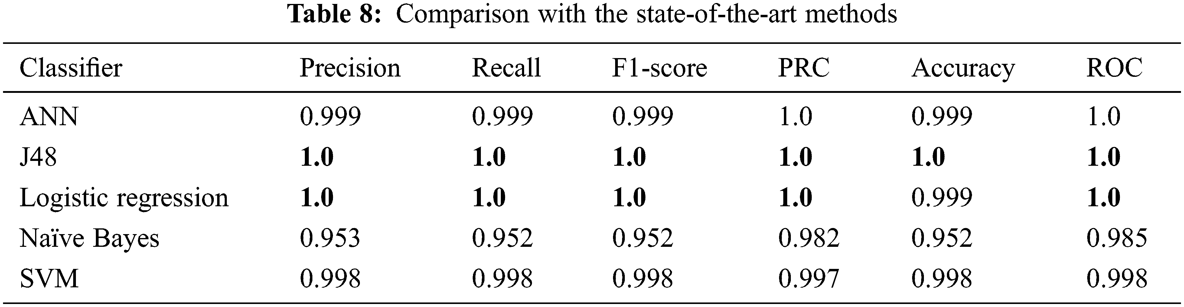
From Tab. 8, one can observe that using the J48 algorithm provides better results as compared to other state-of-the-art methods. Logistic regression achieved much better accuracy (0.999) than Naïve Bayes (0.952). It is worth recalling that SVM performance is put on top of the proposed approaches in our study in terms of Precision. The baseline classifier models generally outperform the proposed methods considerably in most performance measures, particularly in this churn prediction task.
We compare our results for the proposed approaches and the baseline methods with the work by Qureshi et al. [21], which was the only study found so far working with the same Telecom dataset. The comparison shows that our methods achieved significantly better performance. According to Tab. 9, the previous research suffers from reduced sensitivity, particularly for predicting the churn in the dataset. The proposed methods obtained better performance for both accuracy and sensitivity for predicting the churn.

The best accuracy of 0.75 was obtained with an Exhaustive CHAID algorithm, a variant of the standard decision tree algorithm. We can observe that the recall for churners was 60%, whereas the recall for active customers was 76%. For the Telecom database, the proposed method outperformed the previous work. Therefore, our conclusion from the experimental results is that DL models perform equivalent to the baseline methods, which was confirmed in Umayaparvathi and Iyakutti’s study [6].
The problem of churn has an impact on numerous sectors; telecommunication is one of them. Our attention has been focused on predicting customer churn to improve the decision-making for churn management. This study has mainly focused on deep learning with its algorithms, concentrating on Deep neural networks, Convolution neural networks, and Recurrent neural networks. Moreover, we preprocess the dataset, considering the data imbalance, which affects the model that predicts churn. In this research study, a CNN model was developed to identify the potential churners. This study presented a detailed experimental analysis, proposing a 1D CNN model along with RNN and DNN models for churn prediction. The deep learning models were 96% accurate in the case of DNN, 91% accurate in the case of 1D CNN, and 93% accurate Simple RNN. The main contribution is that we demonstrated a system that can obtain 96% accuracy on churn prediction. Furthermore, we achieve 99% for ROC and Precision-Recall Curve Area Under the Curve for DNN classification in addition to bringing the loss down to 1%. The growing popularity of using Keras for deep learning released a new approach and a direction for solving classification problems and predictions. In this research, various hyperparameters are adjusted and compared. It is discovered that regularization techniques such as early stopping and dropout, besides optimization, affect the network performance. We also perform a comprehensive comparison of deep learning and baseline methods to exploit their respective strengths. In our tasks, deep learning methods outperformed the baseline methods reported in prior work for churn prediction on an identical dataset. One of the most vital points of this approach is handling the imbalanced data, which has shown significant improvements in results.
In the future, we intend applying the approaches identified in this research for predictive modeling problems involving other datasets. Moreover, another open area of research is investigating the application of long short-term memory and Gated Recurrent Units in churn prediction. Moreover, the most essential attributes in predicting churn could be identified using information gain. Once the customers are marked as potential churn, an incentive scheme could be introduced to retain those customers.
Acknowledgement: The researchers would like to thank the Deanship of Scientific Research, Qassim University for funding the publication of this project.
Funding Statement: The authors received no specific funding for this study.
Conflicts of Interest: The authors declare that they have no conflicts of interest to report regarding the present study.
1. C. H. Lovelock, P. Patterson and J. Wirtz, “Services marketing: An Asia-pacific and Australian perspective,” 6th ed., Melbourne, Vic, Australia: Pearson, 2015. [Online]. Available: https://www.amazon.com/Services-Marketing-Asia-Pacific-Australian-Perspective/dp/B07FM442C1. [Google Scholar]
2. S. Yuan, S. Bai, M. Song and Z. Zhou, “Customer churn prediction in the online new media platform: A case study on juzi entertainment,” in Proc. of the 2017 Int. Conf. on Platform Technology and Service (PlatCon), Busan, South Korea, 2017. [Google Scholar]
3. C. Sung, C. Y. Higgins and B. Zhang, “Evaluating deep learning in chum prediction for everything-as-a-service in the cloud,” in Proc. of the Int. Joint Conf. on Neural Networks, Anchorage, AK, USA, pp. 3664–3669, 2017. [Google Scholar]
4. Y. Bengio, “Deep learning of representations: looking forward,” in Proc. of the Int. Conf. on Statistical Language and Speech Processing, Tarragona, Spain, pp. 1–37, 2013. [Google Scholar]
5. R. Prashanth, K. Deepak and A. K. Meher, “High accuracy predictive modelling for customer churn prediction in telecom industry,” in Proc. of the Int. Conf. on Machine Learning and Data Mining in Pattern Recognition, New York, USA, pp. 391–402, 2017. [Google Scholar]
6. V. Umayaparvathi and K. Iyakutti, “Automated feature selection and churn prediction using deep learning models,” International Research Journal of Engineering and Technology, vol. 4, no. 3, pp. 1846–1854, 2017. [Google Scholar]
7. F. Castanedo, G. Valverde, J. Zaratiegui and A. Vazquez, “Using deep learning to predict customer churn in a mobile telecommunication network,” Wise Athena LLC, pp. 1–8, 2014. [Google Scholar]
8. M. Karanovic, M. Popovac, S. Sladojevic, M. Arsenovic and D. Stefanovic, “Telecommunication services churn prediction-deep learning approach,” in Proc. of the 2018 26th Telecommunications Forum (TELFOR), Belgrade, Serbia, pp. 420–425, 2018. [Google Scholar]
9. S. Agrawal, “Customer churn prediction modelling based on behavioural patterns analysis using deep learning,” in Proc. of the 2018 Int. Conf. on Smart Computing and Electronic Enterprise, Shah Alam, Malaysia, pp. 1–6, 2018. [Google Scholar]
10. N. Almufadi, A. M. Qamar, R. U. Khan and M. T. Ben Othman, “Deep learning-based churn prediction of telecom subscribers,” International Journal of Engineering Research and Technology, vol. 12, no. 12, pp. 2743–2748, 2019. [Google Scholar]
11. I. AlShourbaji, N. Helian, Y. Sun and M. Alhameed, “Customer churn prediction in telecom sector : A survey and way a head,” International Journal of Scientific & Technology Research, vol. 10, no. 1, pp. 388–399, 2021. [Google Scholar]
12. H. Jain, A. Khunteta and S. Srivastava, “Telecom churn prediction and used techniques, datasets and performance measures: A review,” Telecommunications Systems, vol. 76, no. 4, pp. 613–630, 2021. [Google Scholar]
13. “Mobile telephony churn prediction dataset,” 2010. [Online]. pp. 31–33. Available at: https://www.customers-dna.com. [Google Scholar]
14. S. R. Dubey, S. K. Singh and B. B. Chaudhuri, “A comprehensive survey and performance analysis of activation functions in deep learning,” arXiv preprint, arXiv:210.14545, 2021. [Google Scholar]
15. A. Mustapha, L. Mohamed and K. Ali, “Comparative study of optimization techniques in deep learning: application in the ophthalmology field,” Journal of Physics: Conference Series, vol. 1743, pp. 012002, 2021. [Google Scholar]
16. D. P. Kingma and J. L. Ba, “Adam: A method for stochastic optimization,” in Proc. of 3rd Int. Conf. for Learning Representations,” in San Diego, CA, USA, 2015. [Google Scholar]
17. T. Dozat, “Incorporating nesterov momentum into adam,” in Proc. Int. Conf. for Learning Representations Workshop Track, San Juan, Puerto Rico, 2016. [Google Scholar]
18. S. Sun, Z. Cao, H. Zhu and J. Zhao, “A survey of optimization methods from a machine learning perspective,” IEEE Transactions on Cybernetics, vol. 50, no. 8, pp. 3668–3681, 2020. [Google Scholar]
19. T. Tieleman and G. Hinton, “Lecture 6.5-rmsprop: divide the gradient by a running average of its recent magnitude,” COURSERA: Neural Networks for Machine Learning, vol. 4, pp. 24–31, 2012. [Google Scholar]
20. S. Karsoliya, “Approximating number of hidden layer neurons in multiple hidden layer BPNN architecture,” International Journal of Engineering Trends and Technology, vol. 3, no. 6, pp. 714–717, 2012. [Google Scholar]
21. S. A. Qureshi, A. S. Rehman, A. M. Qamar, A. Kamal and A. Rehman, “Telecommunication subscribers’ churn prediction model using machine learning,” in Proc. Eighth Int. Conf. on Digital Information Management (ICDIM), Islamabad, Pakistan, pp. 131–136, 2013. [Google Scholar]
 | This work is licensed under a Creative Commons Attribution 4.0 International License, which permits unrestricted use, distribution, and reproduction in any medium, provided the original work is properly cited. |