Computer Systems Science & Engineering DOI:10.32604/csse.2023.021469
Article

Machine Learning and Artificial Neural Network for Predicting Heart Failure Risk

Polin Rahman1, Ahmed Rifat1, MD. IftehadAmjad Chy1, Mohammad Monirujjaman Khan1,*, Mehedi Masud2 and Sultan Aljahdali2

1Department of Electrical and Computer Engineering, North South University, Bashundhara, Dhaka, 1229, Bangladesh
2Department of Computer Science, College of Computers and Information Technology, Taif University, P. O. Box 11099, Taif, 21944, Saudi Arabia
*Corresponding Author: Mohammad Monirujjaman Khan. Email: monirujjman.khan@northsouth.edu
Received: 04 July 2021; Accepted: 22 September 2021

Abstract: Heart failure is now widely spread throughout the world. Heart disease affects approximately 48% of the population. It is too expensive and also difficult to cure the disease. This research paper represents machine learning models to predict heart failure. The fundamental concept is to compare the correctness of various Machine Learning (ML) algorithms and boost algorithms to improve models’ accuracy for prediction. Some supervised algorithms like K-Nearest Neighbor (KNN), Support Vector Machine (SVM), Decision Trees (DT), Random Forest (RF), Logistic Regression (LR) are considered to achieve the best results. Some boosting algorithms like Extreme Gradient Boosting (XGBoost) and CatBoost are also used to improve the prediction using Artificial Neural Networks (ANN). This research also focuses on data visualization to identify patterns, trends, and outliers in a massive data set. Python and Scikit-learns are used for ML. Tensor Flow and Keras, along with Python, are used for ANN model training. The DT and RF algorithms achieved the highest accuracy of 95% among the classifiers. Meanwhile, KNN obtained a second height accuracy of 93.33%. XGBoost had a gratified accuracy of 91.67%, SVM, CATBoost, and ANN had an accuracy of 90%, and LR had 88.33% accuracy.

Keywords: Heart failure prediction; data visualization; machine learning; k-nearest neighbors; support vector machine; decision tree; random forest; logistic regression; xgboost and catboost; artificial neural network

1  Introduction

One of the egregious causes of death worldwide is heart disease. In 2015, 17.7 million people died, representing 31 percent of all global casualties, according to the World Health Organization (WHO). Heart failure occurs when the heart is handicapped from pumping sufficient blood to fulfill the body’s needs. Each year, it causes 55,000 deaths. In the United States, 230,000 additional deaths occurred because of its indirect contribution. Approximately 90% of people with advanced heart disease die within a year [1]. According to the most recent evidence from the WHO, 118 287 people died from coronary heart disease in Bangladesh in 2018, accounting for 15.23% of all deaths. Bangladesh is in the 115th position globally, with an age-adjusted death rate of 109.32 per 100,000 people. Heart disease is a financial factor as well. The annual prevalence-based expense varies from $868 to $25,532 in South Korea and Germany for heart failure patients. The overall estimated cost is $126.819 per patient. In the case of developing countries such as Bangladesh, according to the National Heart Foundation of Bangladesh-Package Charge of Cardiac Operation (effective from 01 November 2019): Coronary Artery Bypass Graft (CABG)-2,10,000/-; Atrial Septal Defect (ASD)-1,50,000/-; CMC/PDA (Closed Heart Surgery)-60,000/-; Valve Replacement: 1,45,000 + Cost of the Single Valve & 1,50,000 + Cost of the Double Valve; CABG + ASD/VSD-2,10,000 + 50,000; Intensive Care Unit (ICU) with Ventilator Charge (Per day)-8,000/- etc. [2].

Based on the principle of function approximation, when an algorithm is trained, it can give predictions based on given appropriate output in the case of machine learning. Model relationships and dependencies between the predicted output and input characteristics are the core focus of supervised learning [3]. On the other hand, ANN is a computer system designed to simulate how information is analyzed and interpreted by the human brain. Hence, ANN is a computational model and is based on biological brain network architectures and functions [4].

In order to diagnose heart failure, different methods are approached by medical practitioners. The most widely used method is angiography. The high cost and side effects of angiography are considered as the main limitations to diagnosing heart failure. A chemical called N-terminal pro-B-type natriuretic peptide, which is checked during a blood test, and a chest X-ray for evaluating heart conditions are two other available procedures for diagnosing heart failure. An electrocardiogram (ECG) is used to diagnose heart rhythm problems and heart damage. Other methods include echocardiograms and Computerized Cardiac Tomography (CT) scans. These tests help physicians figure out what is behind the signs and symptoms of heart failure. However, those tests require time as well as are not cost-effective. Some patients’ health conditions are unsuitable for those procedures. This problem inspired the development of an ML-trained model that can predict based on a statistical analysis of some parameters, which is time, cost-effective, and, most importantly, side-effect free. This proposed method is efficient in foretelling the risk of heart failure at an early stage. Some supervised learning classifiers like KNN, SVM, DT, RF, LR used for heart failure prediction are used in this research. This study also used XGBoost and CatBoost to produce a model with excellent stability. Boosting could result in a hybrid model with lower errors by maximizing the benefits and minimizing the drawbacks of the single model. This paper also aims to apply ANN for better precision and accuracy in prediction. The dataset for this paper is available online [5]. This dataset is already used in different papers to find the various classification issues related to heart failure risk with different ML algorithms.

Authors in [5] used Naive Bayes (NB), KNN, ANN, SVM, DT, LR, Ada Boost, RF, and SVM. The accuracy of Naive Bayes is 83%, ANN is 74%, the DT is 74%, LR is 84%, KNN is 76%, SVM is 86%, and RF is 83%. The paper [6] used DT, NB, KNN, and RF algorithms. The accuracy for DT is 80.26%, NB is 88.15%, KNN is 90.78%, and RF is 86.84%. The paper [7] model includes the Ada boost (86.66%), SVM (90.00%), ANN (91.11%), Deep Neural Network (DNN) (93.33%), and RF (81.11%) algorithms. The paper [8] model used linear regression-DT-gradient boosting, RF, one rule, ANN, NB, SVM algorithm, K-NN; their accuracy is (73.0%–73.8%), 74.00%, 72.9%, 76.0%, 69.6%, 69.0%, 66.4%. This model [9] used RF, One Rule, LR, NB, and the DT algorithm. Their RF accuracy is 89.14%, their DT is 93.19%, their LR is 87.36%, and their SVM is 92.30%. This [10] model used DNN, RF, Light GBM, and LR algorithms. This model [11] employed RF, DT-AdaBoost (88%), and SVM (90%). This model [12] uses decision linear-SVM and Linear Discriminant Analysis (LDA). Their accuracy is 90%. SVM (83%), aDT (79%), LR (78%), and K-NN (87%) were used in the paper [13]. The paper [14] used Principal Component Analysis (PCA) and Local Binary Pattern (LBP) (98%) for feature extraction and Probability Neural Network (PNN) (95%) for classification.

Modeling survival for heart diseases is still a challenge to this day. The majority of the models created for this purpose are only somewhat accurate with lower accuracy, and also, the predictive factors are difficult to understand. Other papers work on heart diseases, but there are different types of heart disease, and each diagnosis necessitates its own modeling. Visualizing every feature of the dataset helps proper understanding of the entire parameters which are involved. Some studies approach data mining techniques, but detailed visualization of each data field is not well described. Analyzing other methods, the majority are limited to supervised ML classifiers. Neural network and boosting methods are applied everywhere, but more accurate models are also feasible. Although it’s about disease diagnosis, predicting model accuracy is a significant measure of model validation.

This proposed system has been developed to identify people with heart disease, primarily focusing on heart failure risk prediction. This research paper uses all possible supervised algorithms that provide better accuracy and applies boosting algorithms to make them robust. This research also works on data visualization and feature selection algorithms for model training. This paper is a combination of supervised ML, boosting algorithms, and ANN. This paper researched a more optimized model, which provides a better accuracy level than other proposed models. This study also applies a CatBoost algorithm for the first time to heart disease perdition.

Section 1 provides an introduction. In Section 2, materials and methods are discussed. Results and analysis are presented in Section 3. Section 4 concludes the paper.

2  Materials and Methods

2.1 Introduction

In this section, all technical materials and methods are described, including the methodology of the proposed ML model, block diagram, and equations for building the ML model.

2.2 Dataset

This research used the dataset from Kaggle. This dataset contains 12 attributes. To predict mortality from heart failure, this research used those attributes. The feature names are high blood pressure, smoking, sex, anemia, diabetes, platelets, creatinine phosphokinase, serum sodium, age, serum creatinine, ejection fraction, and time [15]. In addition, it contains death events as target variable 0 or 1. This dataset is clean, and there are no missing values in it.

2.3 Block Diagram of Proposed Model

ML models are files that are prepared to understand different types of patterns. It can train a different type of model using an algorithm so that it learns from data. When done with train data, after that, use that data to predict [16]. Boosting is a technique for generating a collection of predictors. Learners are taught sequentially in this method, with early learners fitting basic models and then analyzing the data for errors [17]. Not only an input layer with hidden layers, but also an output layer comprised of ANN. It seems to be a completely connected neural network. That’s why ANN is considered a multi-layer network [18]. Fig. 1 shows that the model works in a few breakdown steps. Firstly, it requires a set of some past data as input for learning. Then, the ML model gained knowledge from training using the dataset and an appropriate algorithm.

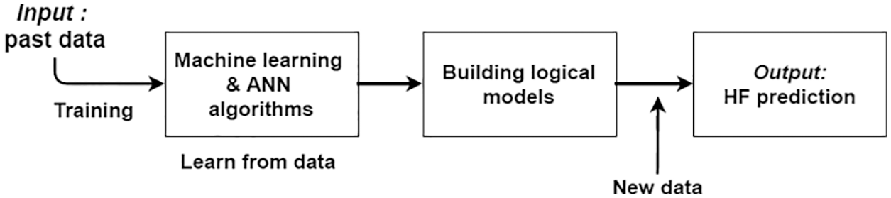
Figure 1: Block diagram of the proposed model

In the training phase, the dataset is required for preprocessing. In the next phase, possible algorithms are used and learn from providing dataset after complement of learning to move to the next phase, the model building phase. Here, the system can build logical models with the help of applied algorithms. Finally, when new data comes to this model, it provides output based on learning from previous data.

2.4 Methodology of Proposed ML Model

This proposed research aims to predict heart failure risk based on ML algorithms and artificial neural ANN. Fig. 2 shows the step-by-step methodology of the proposed model. We work with the dataset; then, data visualization techniques are used in this research paper to understand the data and its correlation better. To select the features, they used the Extra Tree Classifier to determine all the features’ importance. This technique helps to select features that are beneficial for better accuracy. This paper approached supervised learning, like

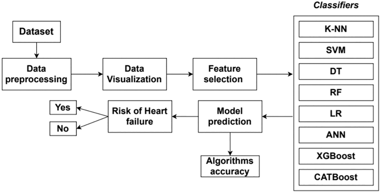
Figure 2: Methodology of the proposed model

KNN, SVM, DT, RF, and LR classifiers, focusing on the dataset’s nature. The XGBoost and CatBoost algorithms are unique algorithms used to supplement the data model’s current results and assist in error correction. These are the ML algorithms used to forecast and fine-tune the results after being trained. And finally, ANN is applied for better prediction. After completing model training with the training dataset and all classifiers, the model can give a prediction. Based on the provided parameters, it will provide a binary classification of whether a person has a risk of heart failure or not. The model accuracy of each applied classifier is calculated with a confusion matrix done for this research.

2.5 Data Visualization

The data comes from a report on cardiovascular diseases that tracked 12 different patients’ criteria and showed whether they were at risk for heart disease [15].

2.5.1 Statistical Analysis

Age Distribution: The dataset’s mean age is over 65 years old, with a minimum age of 42 and a maximum of 95. This makes more sense, given that cardiovascular disease mainly affects people in their later years.

Gender Distribution: This dataset contains 62 males and 34 females. This equates to 64.5 and 35.5 percent, respectively. It is possible that males are more vulnerable to cardiovascular diseases (CVDs) and that having a CVD was a requirement for participants in the research.

2.5.2 Risk Factors

Fig. 3 shows the distribution plots among smoking, anemia, high blood pressure, and diabetes. The X-axis represents the follow-up period (days), while risk factors are shown on the Y-axis. The top four rows of the plot represent patients who had each risk factor, while the bottom four rows represent patients who did not. Of the group of people at risk, 48% were anemic, 41% were diabetic, 31% had high blood pressure, and 31% were smokers. (Red: Smoking, Green: Anaemia, Orange: High Blood Pressure, Blue: Diabetes).

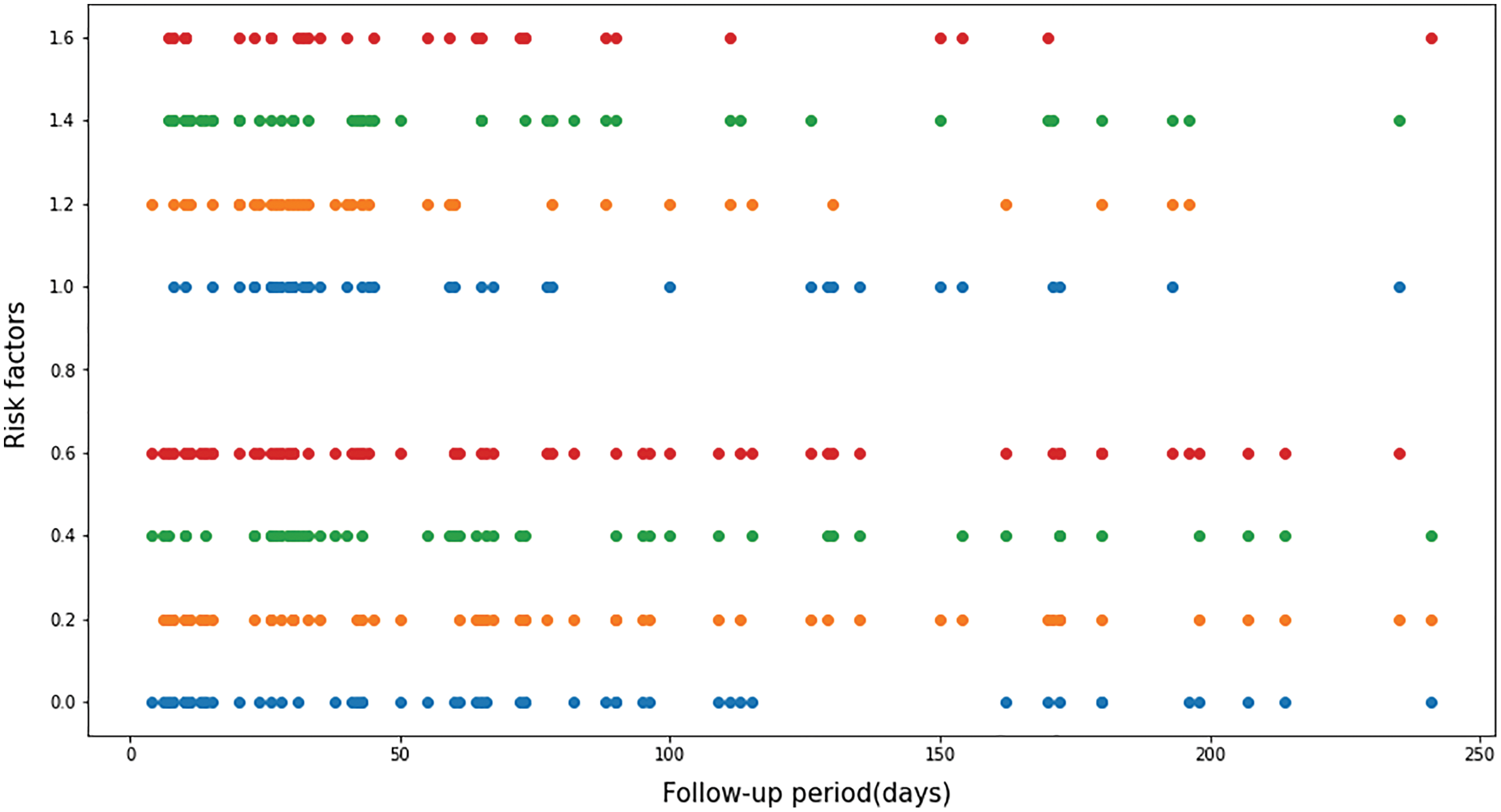
Figure 3: Distribution plots

2.5.3 Blood Test Parameters

Fig. 4 represents the scatter plots of five blood parameters. The X-axis shows the Creatine Phosphokinase (CPK) level, ejection fraction, platelet count, serum creatinine, and serum sodium. The Y-axis represents the follow-up period (days).

a) Creatine Phosphokinase (CPK): It shows that most people’s creatine phosphokinase range is standard with a few high ranges. The X-axis shows the level of the CPK enzyme in the blood (mcg/L), and the Y-axis shows the follow-up period (days). This is the data about the deaths of people who had aCreatine phosphokinase level that was normal. It shows that from the creatine phosphokinase level, we could not guess anything.

b) Ejection Fraction: The percentage of blood leaving the heart at each contraction (percentage) on the X-axis, and the Y-axis represents the follow-up period (days). Most of the patients die within 120 days; their ejection fraction is lower than 45%. The normal range is 50% to 70%, below the normal ejection fraction range, causes potential heart failure.

c) Platelets Count: The platelets in the blood (kilo platelets/mL) in the X-axis and the Y-axis shows the follow-up period (days). This data shows that most patients’ platelet counts are in the normal range between 150 and 400 k. So that is not a factor in heart failure.

d) Serum Creatinine: The serum creatinine level in the blood (mg/dL) is on the X-axis, and the Y-axis shows the follow-up period (days). Most patients’ serum creatinine is lower than usual, and low serum creatinine is the reason for heart failure.

e) Serum Sodium: The X-axis represents the serum sodium level in the blood (mEq/L), and the Y-axis represents the follow-up period (days). Most of the patient’s serum sodium is in the normal range between 135 and 145. Some patients have serum sodium levels below the normal range. So, serum sodium is not a perfect way to detect potential heart failure.

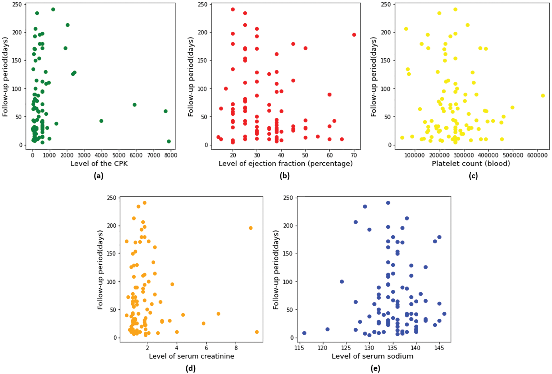
Figure 4: Scatter plots of blood test parameters

2.6 Feature Selection

The extra trees algorithm works by creating a large number of DT that hasn’t been trimmed. In the case of regression and predictions, both are formed by averaging the forecasts of the DT. The Extra Tree Classifier is used for feature selection. It uses majority voting in the case of classification [19].

Fig. 5 shows the feature name vs. feature importance graph. The X-axis of this graph represents features’ importance level, and the Y-axis represents feature names.

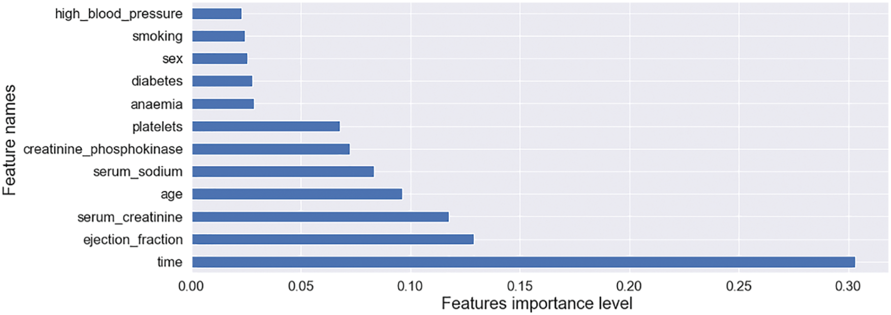
Figure 5: Feature name and their importance graph

This feature importance graph is generated using the Extra Tree classifier for this research to figure out the substantial impact on features of a model train. The impact on features is substantial, exemplarily: time, ejection fraction, serum creatinine, age, serum sodium, creatinine phosphokinase, platelets, diabetes, anemia, sex, and high blood pressure [15]. This research selected time, ejection fraction, and serum creatinine as features.

2.7 Classifiers

2.7.1 K-NN

K-NN has many forms; this is why it can be verified by other ML algorithms. Furthermore, it is non-parametric, making K-NN more effective than other algorithms, which are parametric [20].

Euclidean:

∑i=1k⁡(Xi−Yi)2 (1)

2.7.2 SVM

SVM is also a supervised algorithm that is also used for classification and regression problems. For example, it is in classification to find the hyperplane after verifying their two classes [21].

Maximizing the margin:

WTx+b=0 (2)

where W = weight vector

B = bias

Calculate the margin:

(X+−X−).W=(X+−X−).W||w||=X+.W||W||−X−.W||w|| (3)

Cost function and gradient update:

L(w)=∑i=1⁡max(0,1−Yi[WTXi+b])+λ||W||22 (4)

2.7.3 DT

DT algorithms are a subclass of supervised type algorithms. DT for creating training models can predict any target variable by learning DT rules [22].

Entropy:

E(s)=∑i=1c−Pilog2Pi (5)

(s)=∑i=1c−Pilog2 (6)

E(T,x)=∑c∈x⁡P(c)E(c) (7)

Information gain:

Informationgain(T,X)=Entrophy(T)−Entrophy(T,X) (8)

Gini index:

Gini=1−∑i=1c⁡(Pi)2 (9)

Gain ratio:

Gain ratio = Information gain/split info

Variance:

Variance=∑⁡(X−X”)2n (10)

Chi square:

x2=∑(O−E)2E (11)

2.7.4 RF

The RF algorithm is also a supervised algorithm. Typically, the RF algorithm makes DT on data samples, then it receives a prediction one by one, and lastly, it chooses the perfect solution by voting [23].

MSE = MSE=1N∑i=1N⁡(fi−yi)2 (12)

where N is the number of data points,

Fi is the value returned by the model.

Yi is the actual value of data point i.

2.7.5 LR

LR is a model of probabilistic statistical classification. Different regression from the linear output of logistics regression sample probability is either positive or negative. It depends on the linear measurement of the sample [24].

Log[y1−y]=b0+b1X1+b2X2+b3X3+…+bnXn (13)

2.7.6 ANN

The neural network is a way of creating a brain model. This algorithm’s fundamental goal is to build a method that works better than the previous system. ANN randomly takes some predictions, compared with the correct ones, and the error one is calculated [18].

Calculate the dot products:

X.W=X1.W1+X2.W2+X3.W3+b (14)

Summation of the dot product:

f(x)=11+e−(x) (15)

Back propagation:

Calculate the cost:

MSE=1n∑i=1n⁡(Y′i−Yi)2 (16)

To minimize the cost:

∗Wx=Wx−a(∂Error∂Wx) (17)

where, *wx = New weight

Wx = old weight, A = learning rate

( ∂Error∂Wx ) = with respect to weight

2.7.7 XGBoost

Gradient boosting is a perfect tool for supervised learning, and it works on classification, regression, and ranking. It is an implementation of generalized grading boosting. It has excellent performance on predictive, highly optimized multicore [25].

∑j=1p−1⁡[Xσj,k=Xσp,k]Yσj+a.p∑j=1p−1⁡[Xσj,k=Xσp,k]+a (18)

2.7.8 CatBoost

Catboost is a DT gradient boosting algorithm. It is widely open-source and is easy to use. It has a couple of boosting nodes. One is ordered, and the other is plain [26].

jm(∅m)=∑i=1n⁡L(yi,f(m−1)(Xi)+∅m(Xi)) (19)

2.8 Tools and Modules

Python, a specially dedicated high-quality ML language, is used for this proposed model. Several library packages and modules, such as Scikit-learns, Pandas, NumPy, Seaborn, Matplotlib, are used for ML models, and TensorFlow, Keras, is used for neural network model training. The ML library Scikit-learn has a huge scale for clustering, regression, and classification algorithms. Classification algorithms are used for this research purpose. The Pandas module is used for reading data from a wide range of sources, like Comma-Separated Values (CSV). NumPy is used for adequate container storage, which is highly required for generic multi dimensional data. For this research purpose, complete quality visualization and two-dimension (2D) graph plots are required, which Seaborn and Matplotlib libraries do. An end-to-end ML library such as TensorFlow is required for the proposed neural network model. Keras, another leading Python library, is also necessary for this proposed model because it includes neural network algorithms for normalization, optimization, and activation layers. The Jupyter Notebook is used for data handling, statistical modeling, model training, and analysis.

3  Results and Analysis

3.1 K-NN ModelAccuracy

Import “K Neighbor Classifier” from scikit-learn to train this model with KNN. Select neighbors ranges between 3 and 10, and finds the most accurate score, as shown in Fig. 6.

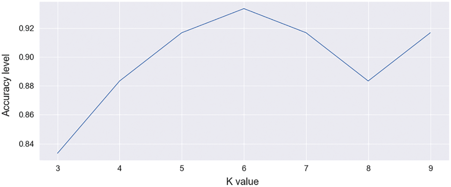
Figure 6: Accuracy score graph of KNN [range between 3–10]

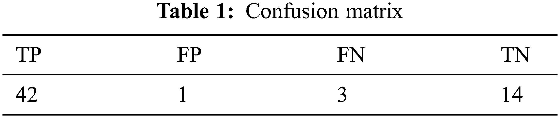
This accuracy score graph shows the K value on the X-axis and the accuracy level on the Y-axis. It is also shown that the value of K = 6 provides height accuracy. The number of neighbors you choose: 6 [K = 6] provides 93.33% accuracy. The confusion matrix is shown in Tab. 1. It predicts 42 data as TP (True Positive) from the test data and 14 data as TN (True Negative). It predicts one data point as FP (False Positive) and provides three data points as FN (False Negative).

3.2 SVM Model Accuracy

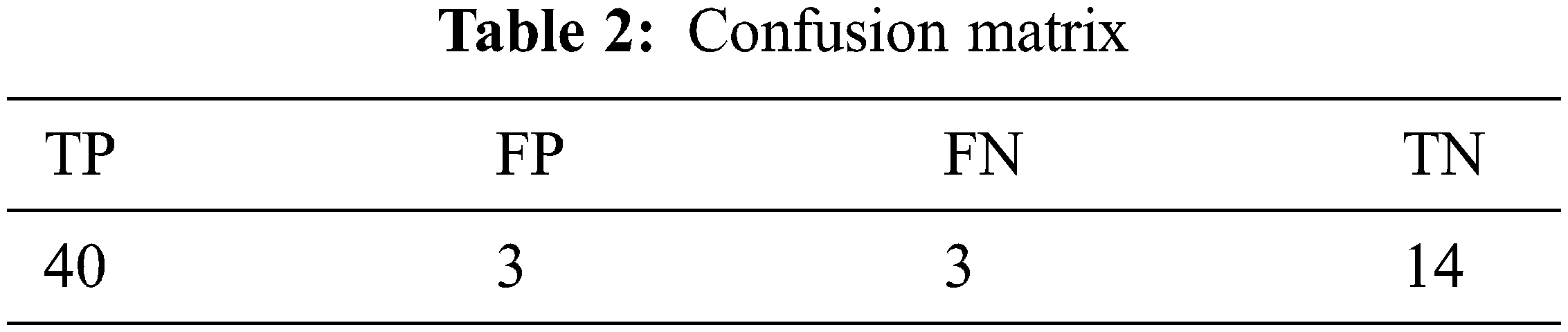
FN. Import SVC from scikit-learn to train this model. Finding C values in the range of 0.5–1.0 is shown in Fig. 7. This graph shows C values on the X-axis and accuracy levels on the Y-axis. To avoid each train data misclassifying, SVM optimization allows C parameter. Selected C = 0.6 and random state = 0, it provides 90.00% accuracy. The confusion matrix is shown in Tab. 2. It predicts 40 data points as TP and 14 data points as TN. It predicts 3 data points for FP and provides 3 data points for negative FN.

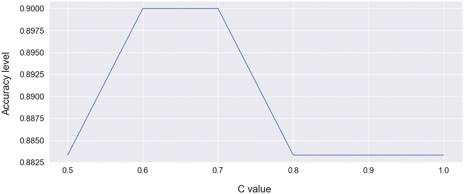
Figure 7: C value select curve for SVC [range between 0.5–1.0]

3.3 DT Model Accuracy

For this research purpose, we imported a DT classifier from the scikit-learn library. The DT classifier requires the maximum number of samples for each node, and the limit of tree growth depends on the max-leaf node hyper parameter. The random state value is selected as 0, which ensures that the model always provides the same output. Max leaf node with the corresponding accuracy is shown in Fig. 8.

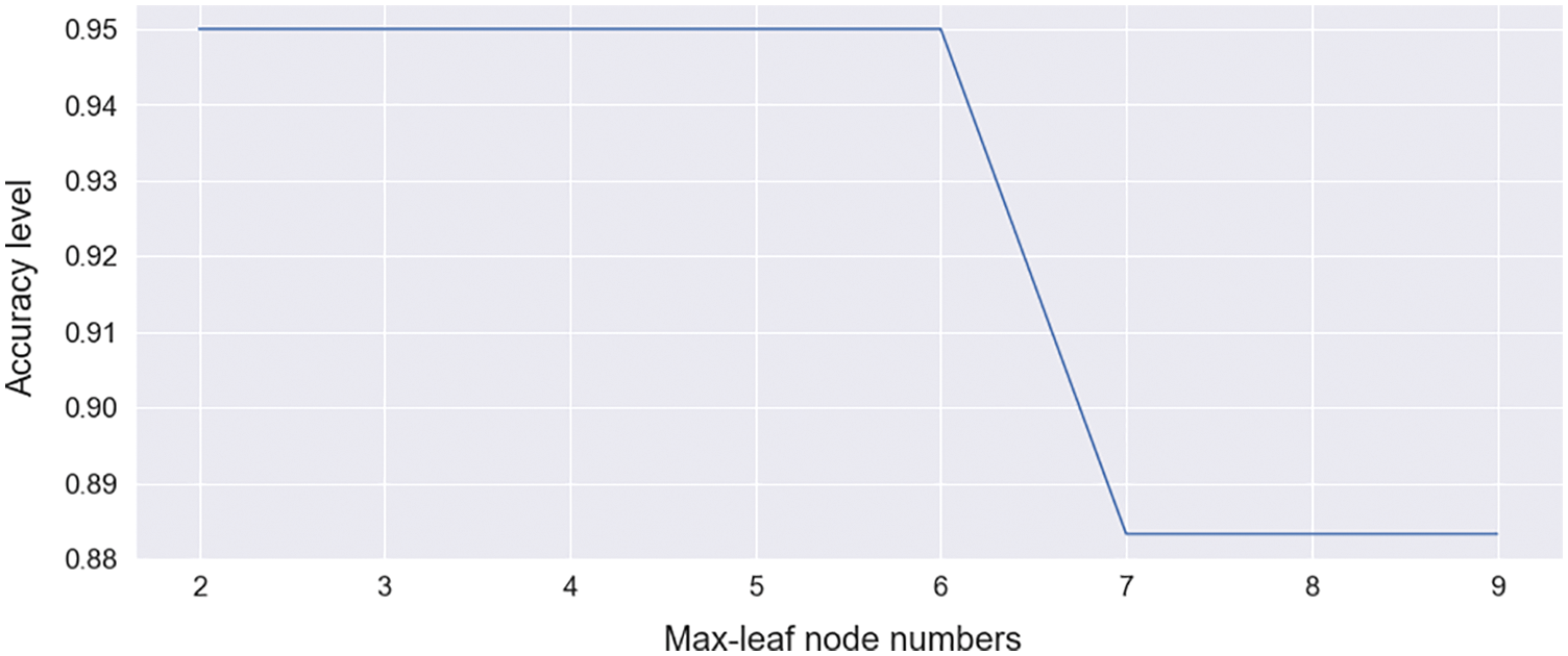
Figure 8: Max leaf node select curve for DT [range between 2–9]

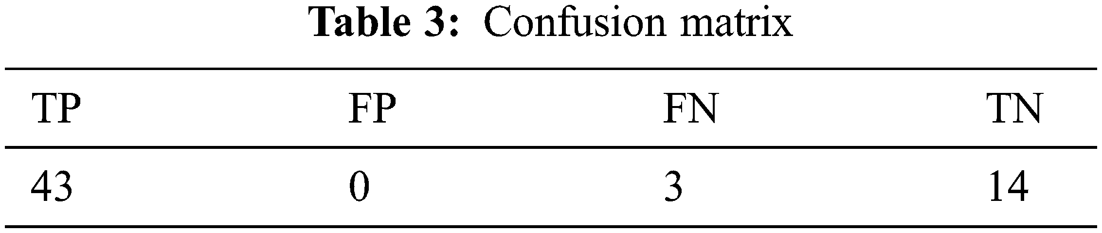
In this graph, the X-axis represents the max-leaf node number, and the Y-axis represents the corresponding accuracy of the model. This graph shows that rings 2–6 provide the highest accuracy. To ensure the highest accuracy, select max-leaf node = 3, and it provides 95% accuracy. A confusion matrix is shown in Tab. 3. This model predicts 43 data as TP and also 14 data as TN. This model does not wrongly predict negative data as positive and predicts three data as FN.

3.4 RF Model Accuracy

Import the RF classifier from scikit-learn for model training. The random state hyperparameter is selected as 0 for each time similar output by the model. The number of trees developed by the algorithm before taking the complete vote or average prediction is given by another hyperparameter n estimator. Typically, the projection becomes more robust as the number of trees increases; it improves efficiency, slowing down computation. N estimators’ range curve is shown in Fig. 9.

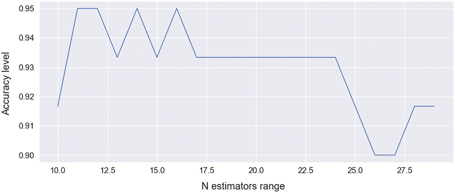
Figure 9: N estimators curve for RF [range between 10.0–27.5]

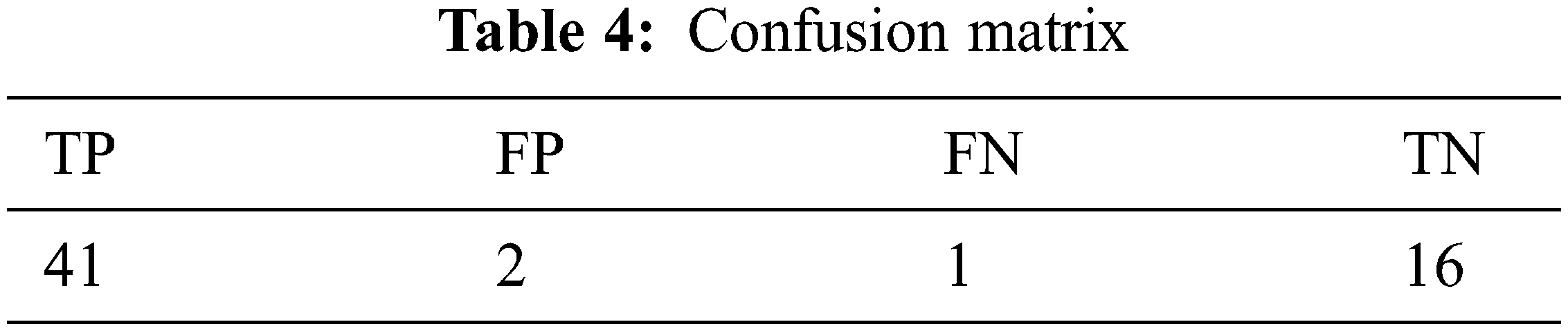
The N estimators range is shown on the X-axis, and the corresponding accuracy is shown on the Y-axis in this graph. It shows maximum accuracy at point 11. With n estimators = 11, this model provides 95% accuracy. The confusion matrix is shown in Tab. 4. This predicts 41 data points as TP from test data and 16 data points as TN. It predicts 2 data as FP and predicts 1 data as FN.

3.5 LR Model Accuracy

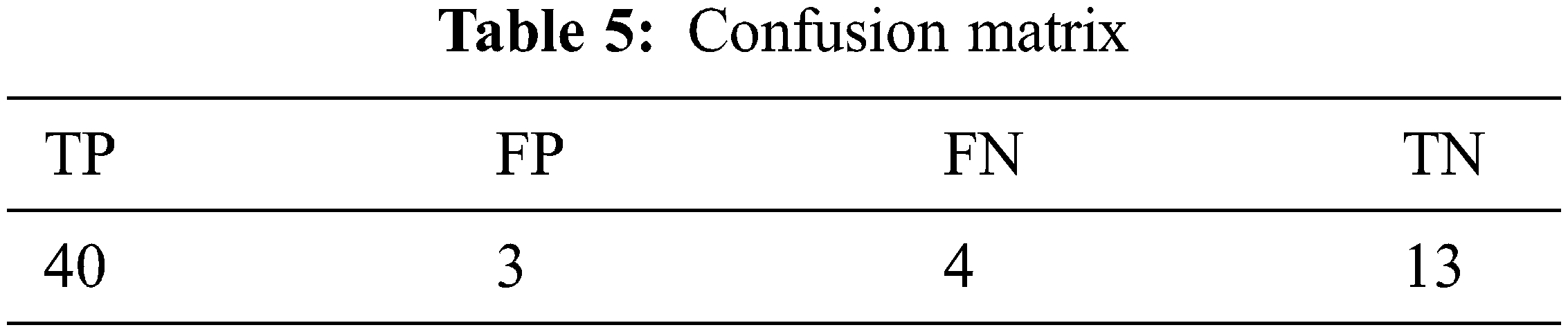
For this study, the library scikit-learn was used to perform LR. Import the model, then have data to deal with, and, finally, perform the necessary transformations. The data was used to match a regression model that was developed. After that, assess the model’s performance and see if it is up to estimating the confusion matrix. Finally, this learned model was used to make predictions, and it was found to be accurate to the tune of 88.33%.The confusion matrix is shown in Tab. 5. From the test results, it predicts 40 data points as TP and 13 data points as TN. It forecasts 3 as FP and 4 as FN.

3.6 ANN Model Accuracy

The batch size is a hyperparameter. This hyperparameter is marked by the number of samples processed. This model selects a batch size of 32. The number of epochs is known as the hyperparameter. It has controls on how many times the learning algorithm will be run. It uses the entire testing dataset for algorithm learning. For example, every sample in the training dataset has had one epoch to change the internal model parameters. Thus, there are one or two batches in an epoch. This model selects 100 epochs for the training dataset. This model obtains 90% accuracy. The confusion matrix is shown in Tab. 6. It predicts 40 data points for TP from test data and 14 data points for TN. It also predicts three negative data points for FP and provides three data points for FN.

3.7 XGBoost Model Accuracy

Import XGBClassifier from xgboost to train the model. Select max depth = 12 and subsample = 0.7, which is the same as the GBM subsample. The n estimators’ argument of the XGBClassifier or XGBRegressor class specifies the number of trees (or rounds) in an XGBoost model. N estimators’ range curve is shown in Fig. 10.

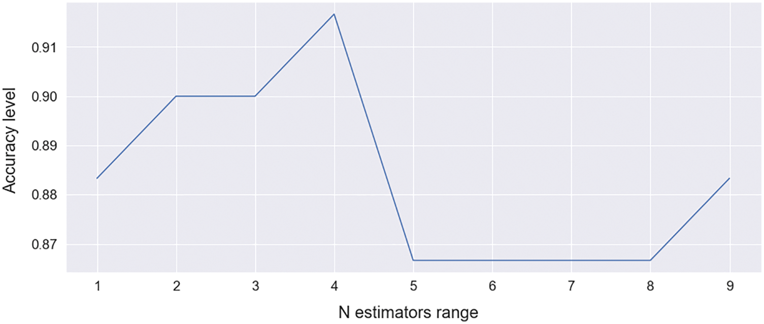
Figure 10: N estimators curve for XGBoost

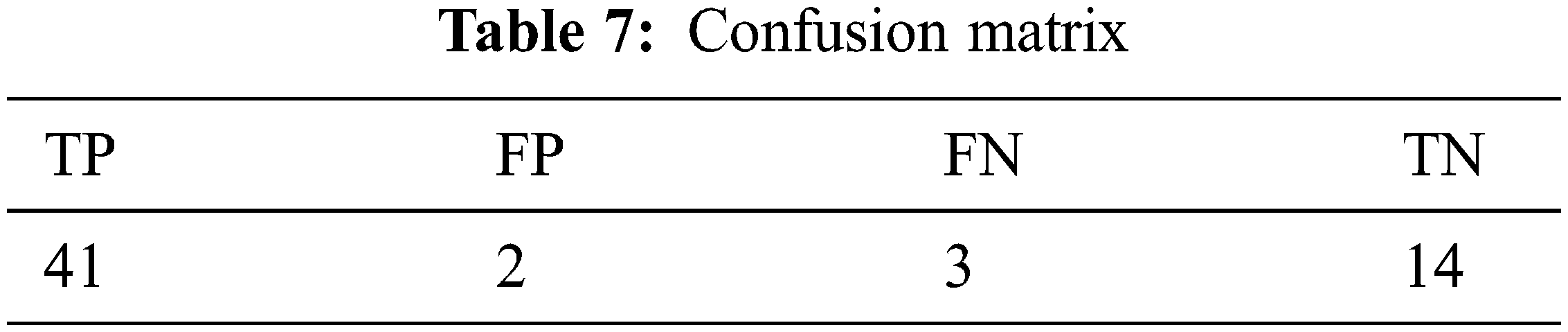
The N estimator range is shown on the X-axis, and the corresponding accuracy is shown on the Y-axis in this graph. It shows maximum accuracy at point 4. Select n estimators = 4; this model obtains 91.67%. The confusion matrix is shown in Tab. 7. From test results, it predicts 41 data as TP and 14 data as TN. It predicts 2 data as FP and 3 data as FN.

3.8 CATBoost Model Accuracy

Import the CatBoost Classifier from Catboost for model training. CatBoost has some incredible plots that show the increase in error metrics over iterations. Setting the plot as true is an excellent strategy. The default value for n estimators is 100. For data hold and the target value, objects X and Y are mentioned. Bypassing test results, this classifier predicted the result and also stored the actual goal in the expected Y. During model training, this classifier achieved 90% accuracy. The confusion matrix is shown in Tab. 8. 40 data predicted as TP from test data and 14 data predicted as TN. It also predicts 3 data to FP and provides the prediction of 3 data to FN. Fig. 11 shows the vertical comparison graph of final model training accuracy using KNN, SVM, DT, RF, LR, ANN, XGBoost, and CATBoost classifier algorithms. The X-axis represents classifier models, and the Y-axis represents the accuracy percentage after model training. All applied classifiers and their corresponding accuracy are shown in Tab. 9.

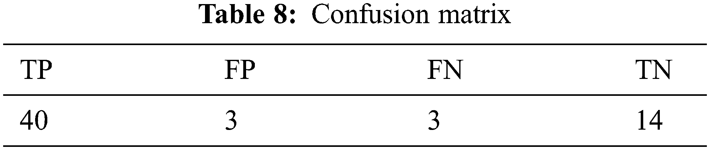
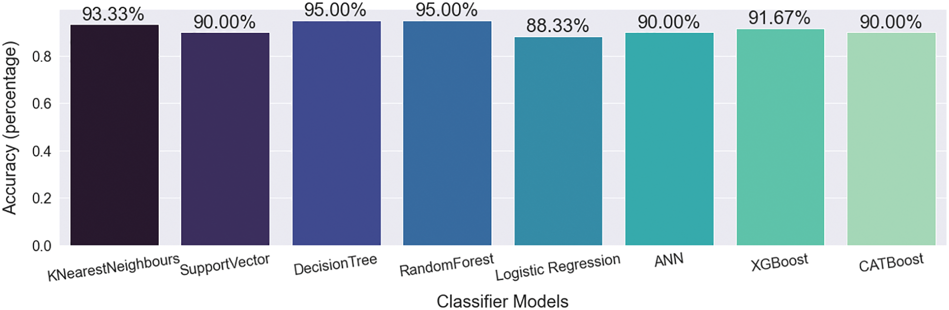
Figure 11: Classifiers comparison graph

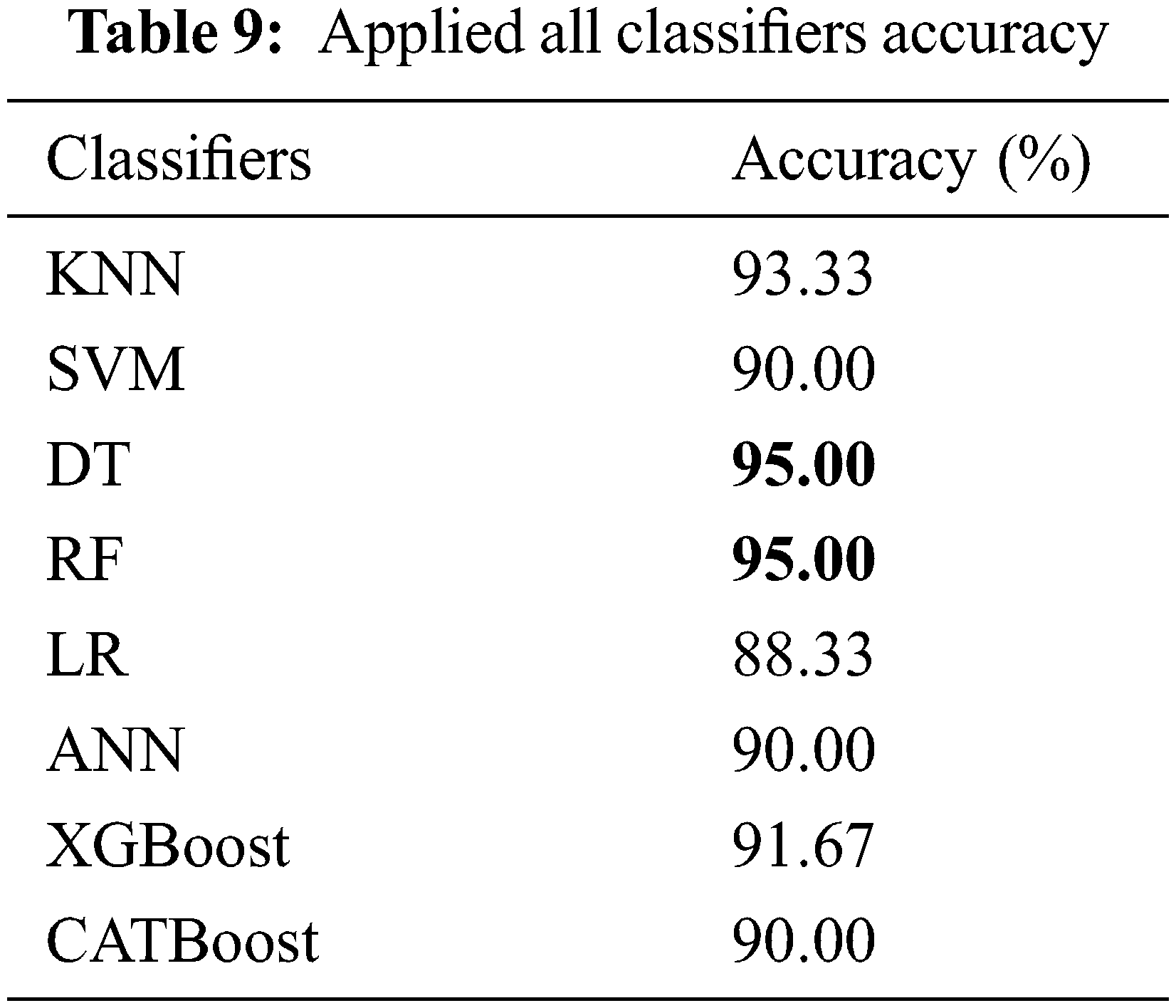
Fig. 11 and Tab. 9 show that this proposed method achieved a height accuracy of 95% with DT and RF classifiers and 93.33% obtained as second height accuracy with KNN. XGBoost got a gratified accuracy of 91.67, SVM, CATBoost, and ANN got 90% accuracy, and LR scored 88.33% while improving the training accuracy. Details of other methods, their accuracies, and comparison with these proposed methods and classifiers’ accuracies are shown in Tab. 10.

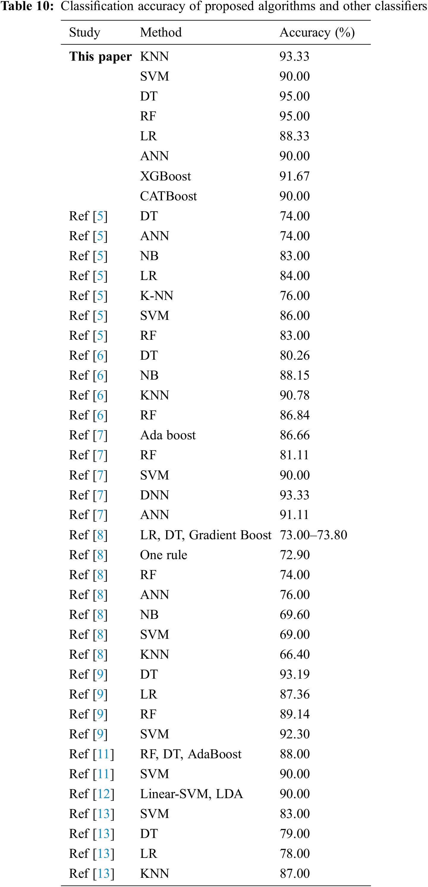
This proposed system in this paper implements eight algorithms with three variations, like supervised ML, boosting, and neural network classifier compared to the other proposed methods. This paper achieved overall maximum accuracy comparatively. Numerous algorithms were applied by [5] and [8], but they obtained an accuracy range of 66.40%–86%. Studies [7] and [9] show that applied methods hold greater accuracy, but their applied algorithms are four to five. Studies [6,11], and [13] approached a pretty similar approach. Their obtained accuracy is not more than 90.78% and 79% of their minimum achievements. In [12], only two models were approached with 90% accuracy. Finally, a study [14] obtained 95% accuracy. This research focused on that algorithm and success with maximum accuracy of 93.33%–95%. Two boosting algorithms were applied more than others, and the boosting approach performed up to 91.67%. Only LR gets 88.33%, but this model gets higher accuracy than other LR applications. The proposed models can be applied in other medical diagnosis [27,28].

4  Conclusion

This research study proposed both ML and ANN approaches to predict heart failure risk. This prediction analysis was performed based on 12 cardiovascular diseases (CVDs), and heart failure is a joint event in this disease. This research approached one ML model such as K-NN, three advanced ML models such as SVM, DT, RF, and LR, two boosting algorithms like XGBoost and CATBoost, and one neural network base model such as ANN for classification. The extra tree classifier feature selection algorithm is also used to select the importance of features. The K-nearest model obtained 93.33% accuracy. It is a better-predicted algorithm in the team of accuracy. The SVM also obtains 90% accuracy. DT and RF get a height accuracy of 95%, and ANN obtains 90% accuracy. Only LR scored less than other applied classifiers. It obtained 88.33% accuracy, which is higher than other studies. Two boosting algorithms, XGBoost and CATBoost, scored with 91.67% and 90% accuracy, respectively. This paper approached CATBoost for the first time for heart failure risk prediction and obtained a satisfactory score. The future scope of this research is to study the deep learning method along with more data and deploy this model into web and mobile apps for massive use.

Acknowledgement: Authors would like to thank the Taif University Researchers Supporting Project Number (TURSP-2020/73), Taif University, Taif, Saudi Arabia.

Funding Statement: Taif University Researchers Supporting Project Number (TURSP-2020/73), Taif University, Taif, Saudi Arabia.

Conflicts of Interest: The authors declare that they have no conflicts of interest to report regarding the present study.

This work is licensed under a Creative Commons Attribution 4.0 International License, which permits unrestricted use, distribution, and reproduction in any medium, provided the original work is properly cited.