DOI:10.32604/csse.2023.022716
| Computer Systems Science & Engineering DOI:10.32604/csse.2023.022716 | |
| Article |
Hybrid Flow Shop with Setup Times Scheduling Problem
1Department of Computer Science and Information, College of Science at Zulfi, Majmaah University, Majmaah, 11952, Saudi Arabia
2Mars Laboratory, University of Sousse, Sousse, Tunisia
3Department of Computer Science, Higher Institute of Computer Science and Mathematics of Monastir, Monastir University, Monastir, 5000, Tunisia
4Industrial Engineering Department, College of Engineering, King Saud University, Riyadh, 11421, Saudi Arabia
*Corresponding Author: Mahdi Jemmali. Email: m.jemmali@mu.edu.sa
Received: 16 August 2021; Accepted: 17 September 2021
Abstract: The two-stage hybrid flow shop problem under setup times is addressed in this paper. This problem is NP-Hard. on the other hand, the studied problem is modeling different real-life applications especially in manufacturing and high performance-computing. Tackling this kind of problem requires the development of adapted algorithms. In this context, a metaheuristic using the genetic algorithm and three heuristics are proposed in this paper. These approximate solutions are using the optimal solution of the parallel machines under release and delivery times. Indeed, these solutions are iterative procedures focusing each time on a particular stage where a parallel machines problem is called to be solved. The general solution is then a concatenation of all the solutions in each stage. In addition, three lower bounds based on the relaxation method are provided. These lower bounds present a means to evaluate the efficiency of the developed algorithms throughout the measurement of the relative gap. An experimental result is discussed to evaluate the performance of the developed algorithms. In total, 8960 instances are implemented and tested to show the results given by the proposed lower bounds and heuristics. Several indicators are given to compare between algorithms. The results illustrated in this paper show the performance of the developed algorithms in terms of gap and running time.
Keywords: Hybrid flow shop; genetic algorithm; setup times; heuristics; lower bound
The hybrid flow shop problems (HFSP) are commonly utilized in several sectors like the manufacturing area. Indeed, HFSP is modeling several production systems in different industries such as paper, electronics, cars, chemicals, and semiconductors [1–4].
The two-stage HFSP is a particular case, which is well studied in the literature. This is due to its practical applications, and its theoretical challenging aspect. Plenty of results are provided to solve this problem using heuristics, meta-heuristics, and exact methods. Authors in [5] proposed an efficient exact method to solve the two-stage HFSP. The latter research doesn't achieve the setup times constraint and the time provided to solve the problem is remarkable. The Two-stage HFSP with transportation times is addressed in [6]. In the latter work, several heuristics and exact methods are developed. In the experimental results, it is clear the luck of the big scale class to show the performance of the developed method when the number of jobs is real big. The two-stage HFSP with availability constraint is addressed in [7], and an exact algorithm is proposed. In the latter paper, there is only one machine in stage 1. In addition, only one interval of maintenance for each machine. Authors in [8] solved the problem using a genetic algorithm (GA). Several constructive heuristics are developed in the latter work to apply the genetic algorithm seeking the enhancement of the results. The luck of the development of lower bounds to be used as a measurement of the real performance of the heuristics is remarkable for the latter work.
In [9], the authors proposed an exact solution for the hybrid flow shop under sequence-dependent setup time for stage one. An upper bound utilized Hungarian method is proposed. In addition, the authors proposed three heuristics. The experimental results need to be performed when the author gives more attention to the big scale instances.
The problem with batch processing machines is studied in [10], where a decomposition approach with variable neighborhood search (VNS) is developed. Unequal ready times for jobs are considered a constraint for the latter problem. This problem with parallel dedicated machines is addressed in [11], and several heuristics are proposed. The objective was the minimization of the total completion time. Besides, the number of machines is limited to one for stage 1 and two for stage 2. Only two heuristics are developed in the later work.
In [12] authors proposed an approximate solution based on a Branch and Bound exact procedure to tackle the problem of two-stage hybrid flow with dedicated machines. Besides, the authors proposed four constructive heuristics to solve the problem and three dominance priorities. In the experimental results, the instances are generated with a maximum of 100 jobs.
In [13] a new application of the problem of two-stage HFSP is introduced and a heuristic with a local search method is developed and an ant colony optimization algorithm is developed. The bi objectives in the latter search are the total energy consumption and the makespan.
Authors in [14] addressed the problem and proposed a mutant firefly algorithm. Two objectives functions are proposed in the latter work. One of the objectives is the simultaneous ratio for the coming of several parts of products at the stage of assembly. The second objective is the on-time delivery ratio related to the products delivery assignment.
In [15] authors investigated the hybrid flow shop problem (DHFSP) under sequence-dependent setup times. Three sub-problems are involved. The first sub-problem is the allocation of factories for each job. The next sub-problem is to find the job sequence for every factory. The third sub-problem is the allocation of each job at each stage. To test the performance of the proposed solutions authors generated 780 benchmarks in total. In the same context authors in [16], a novel simulated-annealing (NSA) algorithm was proposed to find a reasonable manufacturing assignment in a good running time. Setup times are needed when switching between jobs. Considering the setup times while preparing the schedules of jobs on the machines allows having accurate production planning. To minimize the gap between theoretical points and real-life situations, the setup times are not neglected in this study. The two-stage HFSP with setup times is treated in literature [17–20].
In this study, the two-stage hybrid flow shop problem is addressed. Novel heuristics are proposed. These heuristics are based on the exact solution of the problem of the parallel machine under release and delivery times constraints. In addition, a lower bound allowing the assessment of the performance of heuristics are proposed. The studied problem is an NP-hard problem. It is very important to search for heuristics that give approximate solutions to the problem with acceptable time. In addition, the scale of the problem can impact the performance of the heuristics on time and gap. In this paper, a total of 8960 instances are generated and tested to prove the efficiency of the proposed lower bounds and heuristics. In the literature review, there is a lack of treatment of the big scale of instances to solve the problem. Indeed, the number of jobs reaching 200. The proposed heuristics give a solution easily for the big scale of instances with a satisfying time and gap.
The rest of this paper is structured as follows. Problem presentation is presented in Section 2. The lower bounds are developed and displayed in Section 3. The detailed heuristics are given in Section 4. An experimental study and discussion of results are reported in Section 5. Finally, the summarization of the studied work is presented in the conclusion with future lines.
2 Problem Definition and Proprieties
In this section, the presentation of the problem and its relevant proprieties are presented. In addition, the problem of the parallel machine under release and delivery times constraints as well as some of its characteristics are recalled. This is because of the important role of the latter problem in providing algorithms for the current studied problem. The two-stage hybrid flow shop problem with setup times is stated as follows. We are given a shop composed of two stages C1 and C2 in series, containing m1 and m2 identical parallel machines, respectively. A set J = {1, 2, …, n} of n jobs have to be executed on the machines of the two stages in the following way. A machine of C1 is prepared during a setup time s1,j to be ready for processing a job j during p1, j. After completion the stage 1, an available machine in the second stage C2 is prepared during s2, j to process the job j. All machines and jobs are ready for executing at the first time 0. Preemption is not permitted, and all job characteristics
Example 1:
Let m1 = 2 and m2 = 2. The setup times and processing times for the two stages illustrates in Tab. 1. Fig. 1 presents a feasible solution for example 1, where the makespan is Cmax = 142.
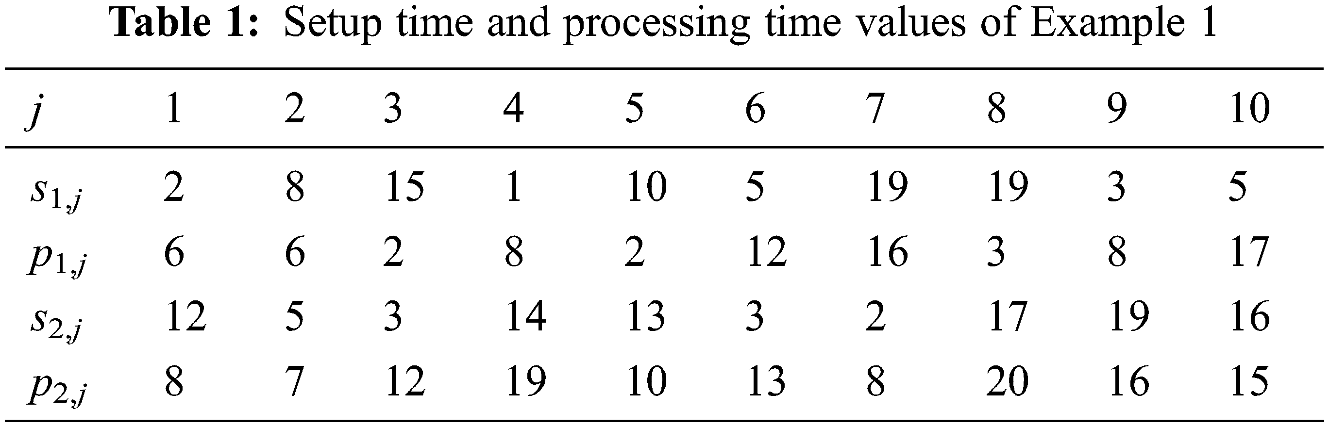

Figure 1: Feasible solution for example 1
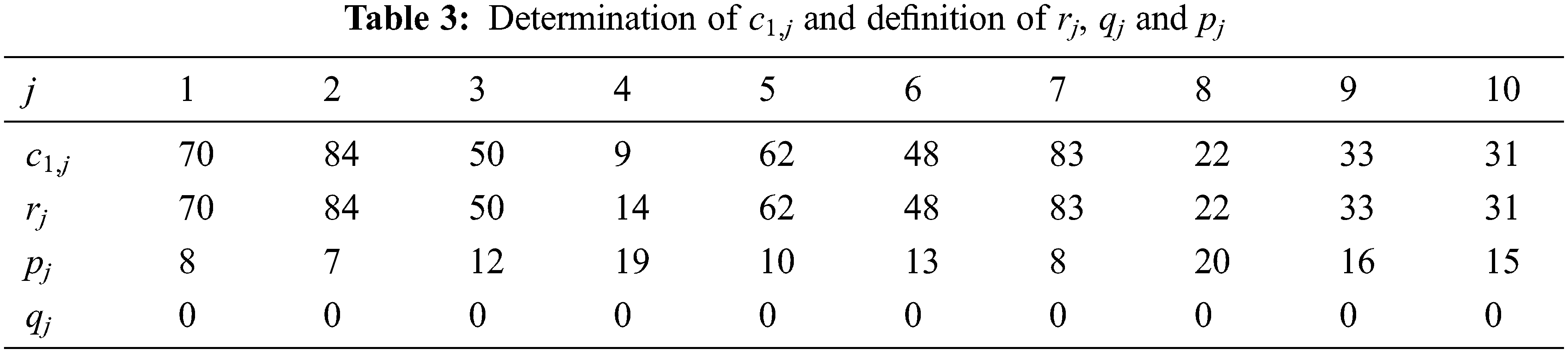
It is remarkable to note that the setup times in stage 1 are connected directly to the processing times, while in stage 2, the setup time might be separated from the processing time, as for job 8. Indeed, for this job c1,8 = 22 which is a release date in the second stage and the setup time is s2,8 = 17 < 22.
In this section, we present three new lower bounds based on the linear relaxation technique. The first one is obtained after applying the relaxation of the second stage using the problem of the parallel machine. The second lower bound is obtained after applying the relaxation of the first stage using the problem of the parallel machine. The third lower bound is an enhancement of the first one.
3.1 Relaxed Second Stage Based Parallel Machine Problem (LB1)
The capacity of the second stage is relaxed and the number of machines m2 is supposed to be not finite. In this case, an ending processing job in stage 1 has no time to wait for processing in the second stage. Consequently, the obtained scheduling problem in stage 1 is a parallel machines problem under release date rj and delivery time qj denoted
▪
▪
▪
▪ m = m1.
Lemma: Any lower bound of the latter defined problem, is a valid lower bound for
Proof:
Remark: The Branch & Bound (B&B) algorithm for
3.2 Relaxed First Stage Based Parallel Machine Problem (LB2)
The capacity of the first stage is relaxed and the number of machines m1 is supposed to be not finite. In this case, for any job a machine is set up at zero time and processes without delay in the first stage. Consequently, the obtained scheduling problem in the second stage is a parallel machine under rj and qj constraints denoted by
▪
▪
▪
▪ m = m2.
Following the same steps as for LB1, the Branch & Bound (B&B) algorithm of
3.3 Enhanced Relaxed Second Stage Based Parallel Machine Problem (LB3)
The capacity of the second stage is relaxed and the number of machines m2 is supposed to be infinite. In this case, an ending processing job in stage 1 has no time to wait for processing in the second stage. Consequently, the obtained scheduling problem in stage 1 is parallel machines problem under rj and qj constraints denoted by
▪
▪
▪
▪ m = m1.
In the same way, and applying the B&B algorithm a third lower bound denoted LB3 is obtained.
Remark: LB3 dominates LB1.
Proof: Clearly, an optimal solution of problem (P1)
Example 2:
In this example, we give the schedule applying LB3 with the same instance presented in Example 1. Now, we solve exactly the
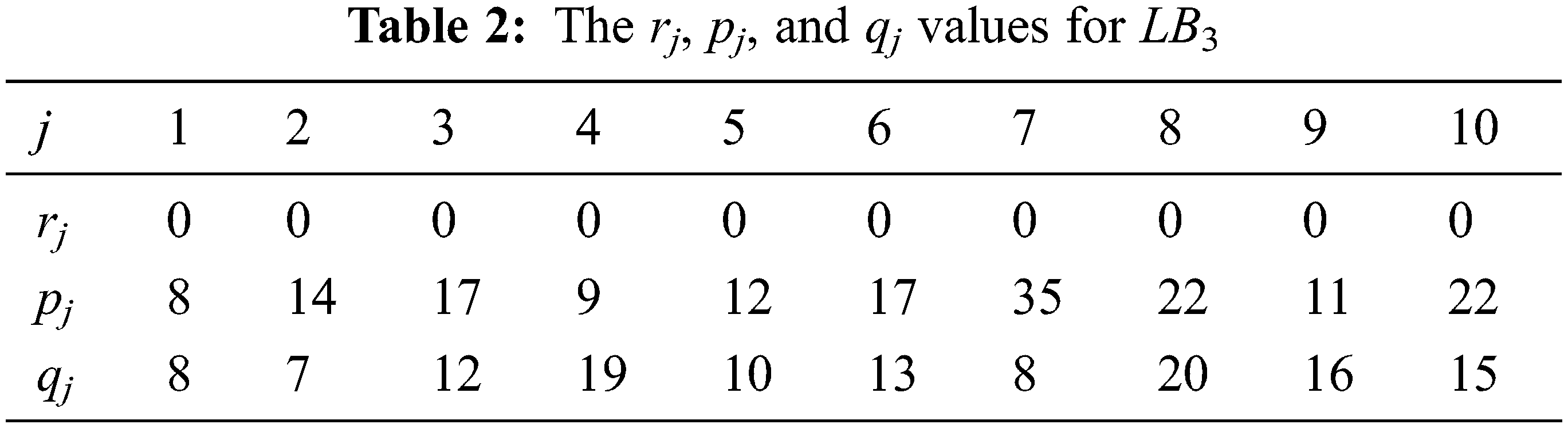
The optimal solution of

Figure 2: Schedule applying LB3
In this section, a metaheuristic and three heuristics are proposed. The developed metaheuristic is implemented using the genetic algorithm (GA). The three other heuristics are based on solving a parallel machines problem under release and delivery time constraints.
John Holland in [23] presented for the first time the genetic algorithms (GAs). The GAs are inspired by natural evolution. Indeed, the main fundamentals of natural evolution in a given environment are memetic. During this process, the chromosomes are the main actors in which all the messages and mutations are performed. The different components are:
1. Chromosome Representation: in this study, a chromosome represents a feasible solution. A chromosome is constituted by a permutation of jobs. The jobs in this permutation are scheduled on the machines of stage 1 according to the most available machine rule. That is, the first remaining job in the permutation is allocated to the most available machine. Once all the jobs are scheduled to stage 1, the jobs are scheduled on the second stage according to the non-decreasing order of their completion time in the first stage.
2. Initial population: All the individuals in the initial population are arbitrarily generated, except one solution which is generated according to the LPT rule in the first stage. The jobs are sorted according to the non-increasing order of their processing time in the first stage. Once these jobs are assigned to stage 1 according to the LPT rule, they are scheduled in the second stage according to the increasing order of their completion time in the first stage.
3. Selection Operator: During the selection phase an operator acts to pick the most suitable solutions in order to accelerate the convergence toward the global optimum. Several operators are utilized and the most used one is the roulette wheel selection rule, which is an adopted selection operator in this study.
4. Reproduction: In this step, an individual passes to the next generation without modification, it is a cloning phase. The main objective of the reproduction phase is to preserve the individuals with high fitness from the actual generation to the next one.
5. The Operator of Crossover: Enriching the diversity of the population is the main objective of the crossover operation. Indeed, in this step, the structure of the individuals (chromosomes) is manipulated. Conventionally, the crossover operator considers two parents and generates two children. To guarantee the innovation (even partially) of the children a crossbreeding is performed. The basic idea is that two successful parents will yield better children. The crossover rate
6. Mutation: The main goal of the mutation is to create a small randomness element in the population of individuals. The mutation operator could increase or decrease the space of the possible feasible solutions, in addition to the variability of the individuals. pm determines the probability of mutating each element (gene) of representation. In this work, the adopted pm is to mutate a percentage of all genes.
7. Replacement Strategies: In this step, individuals are withdrawn following a given selection strategy. Indeed, the best individuals from parents and offspring are kept. This approach allows a rapid convergence and some time to a moderate solution. In order to avoid such a situation, sometimes, bad (fitness) individuals are selected. Those replacement strategies can be deterministic or stochastic.
In practice, the tuple (Population, crossover rate, probability of mutating) considered in the genetic algorithm are chosen as following: (200;0.9;0.9), (200;0.8;0.9), (200;0.9;0.8), (200;0.7;0.9), (200;0.8;0.8), (200;0.6;0.9), (200;0.7;0.8), (200;0.6; 0.8), (200;0.5;0.9), and (200;0.4;0.9).
The heuristic H2 is based on solving optimally a sequence of two parallel machines under release and delivery time constraints. First, a parallel machines problem
▪
▪
▪
▪ m = m1.
Once the above scheduling problem (
▪
▪
▪
▪ m = m2.
In the third step, we remark that the obtained solution is not necessarily a feasible one since it may occur that a job has no setup time in the second stage. To overcome this drawback, an adjusted solution is introduced. The adjustment is as follows. If the first scheduled job in a machine of the second stage is the job j, then we have to check two cases:
1) if s2,j ≥ c1,j then the completion time of j is c2,j = s2,j + p2,j.
2) if s2,j < c1,j then the completion time of j is c2,j = c1,j + p2,j. If a job j is preceded by a job i in the same machine then:
1) if c2,i + s2,j ≥ c1,j then the completion time of j is c2,j = c2,i + s2,j + p2,j.
2) if c2,i + s2,j < c1,j then the completion time of j is c2,j = c1,j + p2,j.
The concatenation of the two feasible solutions respectively in the first and second stages provides a feasible solution for t
Example 3:
We adopt the same instance represented in Tab. 1 in Example 1. In the first stage, we apply
The optimal solution of

Figure 3: Feasible schedule for H2
The heuristic H3 is based on solving optimally a sequence of two parallel machines under release date and delivery time. First, a parallel machine scheduling problem
▪
▪
▪
▪ m = m1.
Once the above scheduling problem (
▪
▪
▪
▪ m = m2.
The obtained solution in the second stage does not include setup times. In this step, the setup times s2,j are embedded before the processing of jobs. The concatenation of the two feasible solutions respectively in the first and second stages provides a feasible solution for the studied problem.
The heuristic H4 is based on solving optimally a sequence of two parallel machines under release and delivery time constraints. First, a parallel machine scheduling problem
▪
▪
▪
▪ m = m1.
Once the above scheduling problem (
▪
▪
▪
▪ m = m2.
In the expression of the processing times pj = s2,j + p2,j we consider the setup time and the processing time as one entity. This will give a feasible solution in the second stage which may largely exceed an optimal solution. To readjust the obtained solution, we split setup time from processing time, and we apply the following recursive rule in the jobs scheduled to the same machine. c2,j = max(c1,j, c2,j−1 + s2,j) where c2,j−1 is the completion time of the predecessor of job j in the same machine. The concatenation of the two feasible solutions respectively in the first and second stages provides a feasible solution for
This section focuses on the illustration and the discussion of the obtained results. All proposed algorithms in this paper were coded in C++. All coded programs were executed by a workstation that has the following characteristics: Intel(R) Xeon(R) CPU E5-2687W v4 @ 3.00 GHz and 64 GB RAM.
The generation of the setup times and processing times are applied according to the uniform distribution denoted by U[st, fi]. In this paper the choice of st = 1 and fi = {20, 40}. The class of instance is depending on the choice of the generation of s1, j, p1, j, s2, j and p2, j. So, we generate s1, j in [1, 20] or [1, 40], and same thing for p1,j, s2,j and p2,j. We denoted by C1, C2, C3, and C4 the choice of fi to generate s1, j, p1, j, s2, j and p2, j, respectively. The value of each variable C1, C2, C3, and C4 represent the manner that the setup times and processing times are generated. For example, if (C1 = 20, C2 = 20, C3 = 40, C4 = 20) meaning that we generate s1,j in [1, 20], p1,j in [1, 20], s2,j in [1, 40] and p2,j in [1, 20]. The number of permutations to generate classes is 42 = 16. The number of machines for each stage is chosen in {2, 3, 4, 5}. The number of permutation to constitute a pair (m1, m2) is 16.
Now, for the number of jobs, we adopt n = {10, 20, 30, 50, 100, 150, 200}. For each type of class (C1, C2, C3, C4), each (m1, m2) and each n we generate 5 instances. Finally, the total number of instances is 16 × 16 × 7 × 5 = 8960.
To assess the performance of the heuristics and lower bounds, the following performance measures are used:
▪ Time: average CPU time (s)
▪
▪
▪
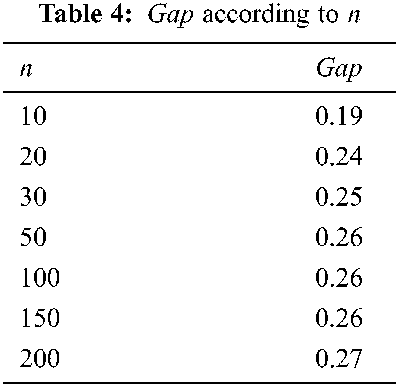
Tab. 4 represents the variation of the
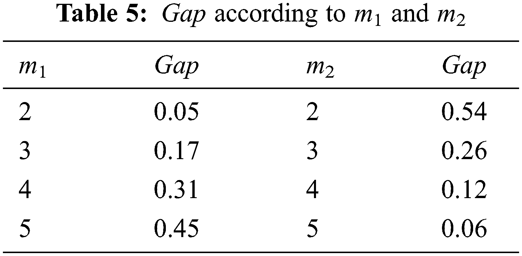
Tab. 5 shows the variation of Gap according to (m1) on stage 1 and to m2 on stage 2.
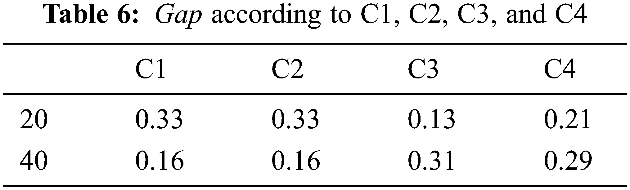
Tab. 6 presents the Gap values according to C1, C2, C3, and C4. The minimum gap value of 0.13 is obtained when C3= 20.
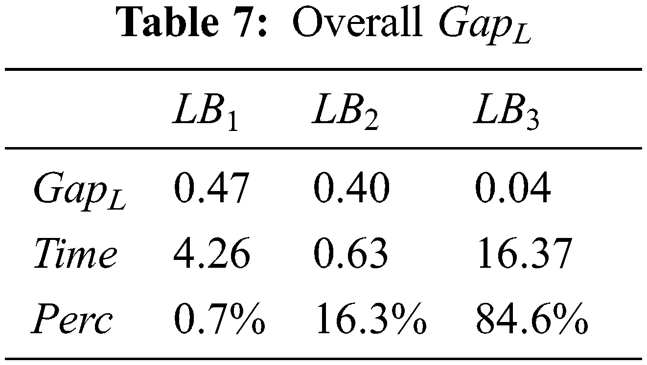
Now, we present the results obtained for the developed lower bounds. Tab. 7 shows that the best lower bound is LB3. Indeed, the percentage of this is lower when the number of instances that LB3 is the best one is 84.6% in an average time 16.37 and an average gap of 0.04.
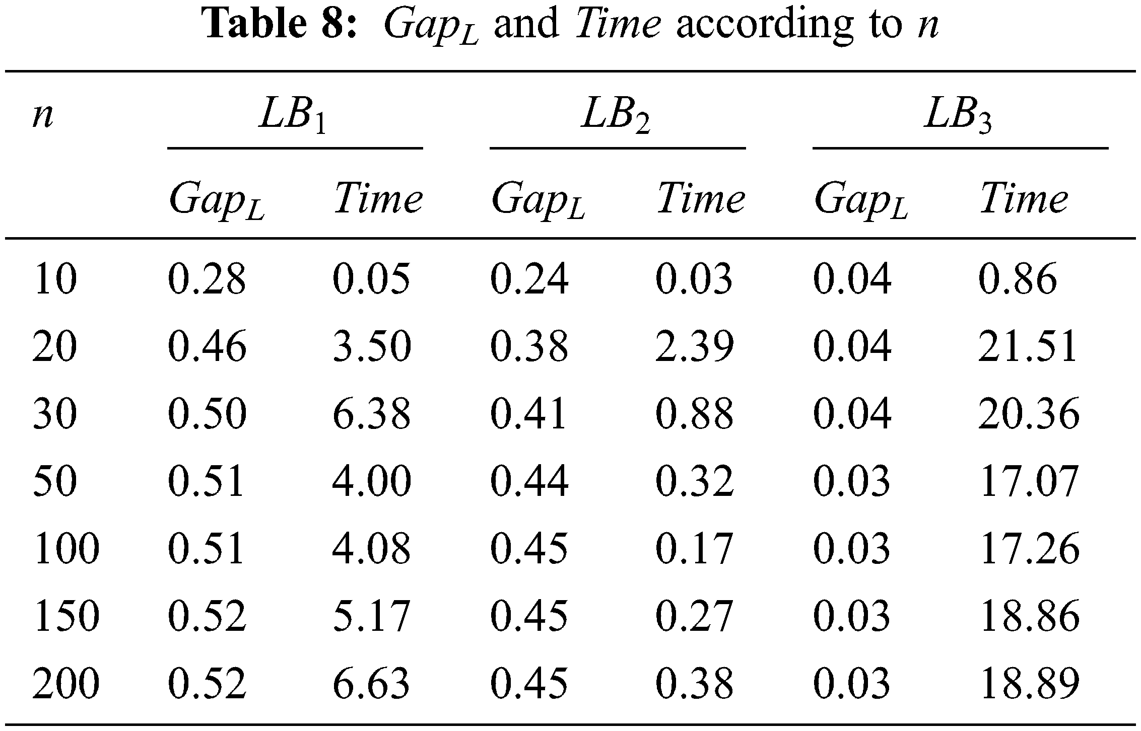
Tab. 8, represents the variation of GapL according to n. For LB3 the maximum gap is obtained when n = {10, 20, 30}.
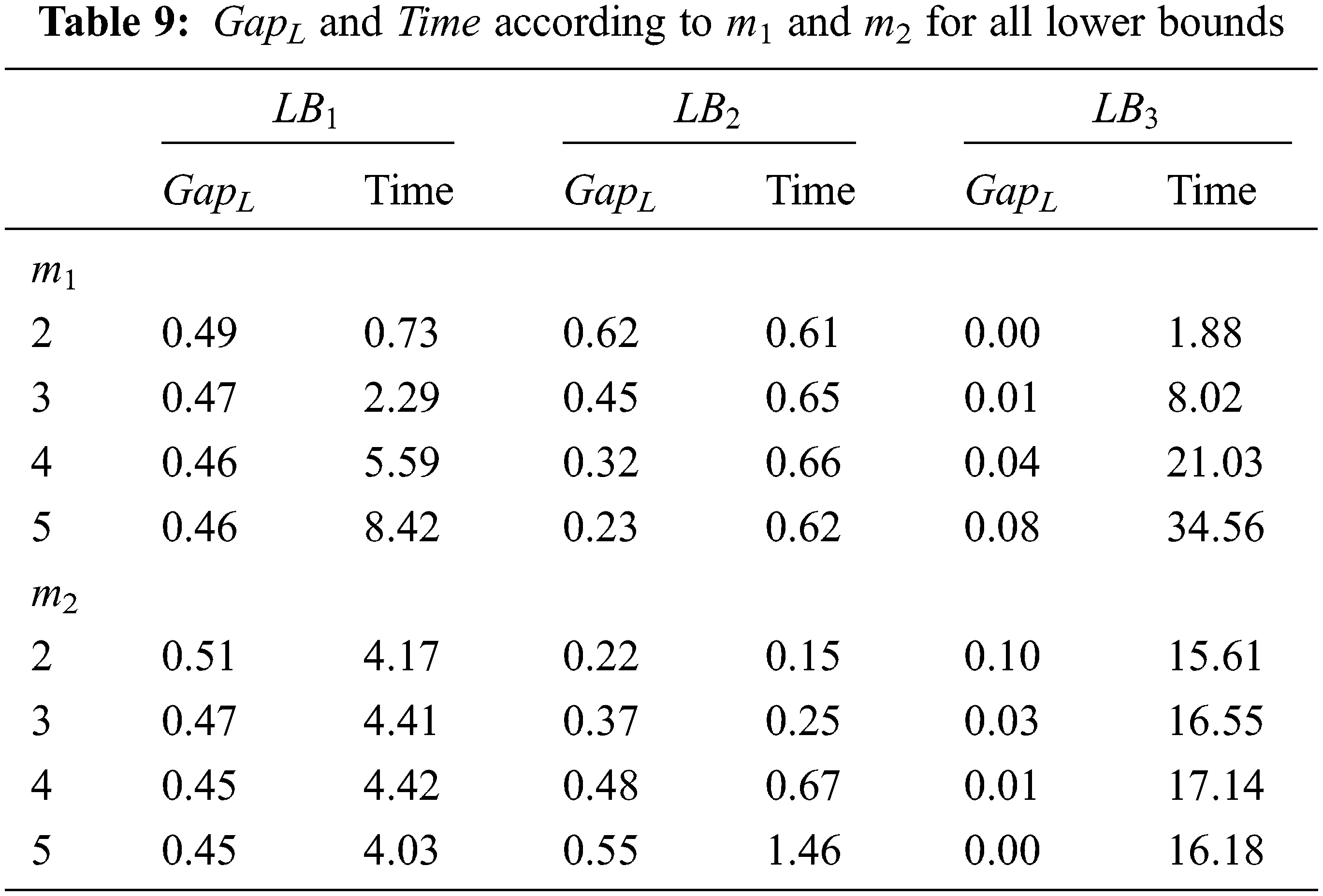
Tab. 9 presents the GapL and Time variation according to m1 and m2 for all lower bounds. The most time-consuming lower bound is LB3 when m1 = 5. In this condition, the running time is reached to 34.56 s.
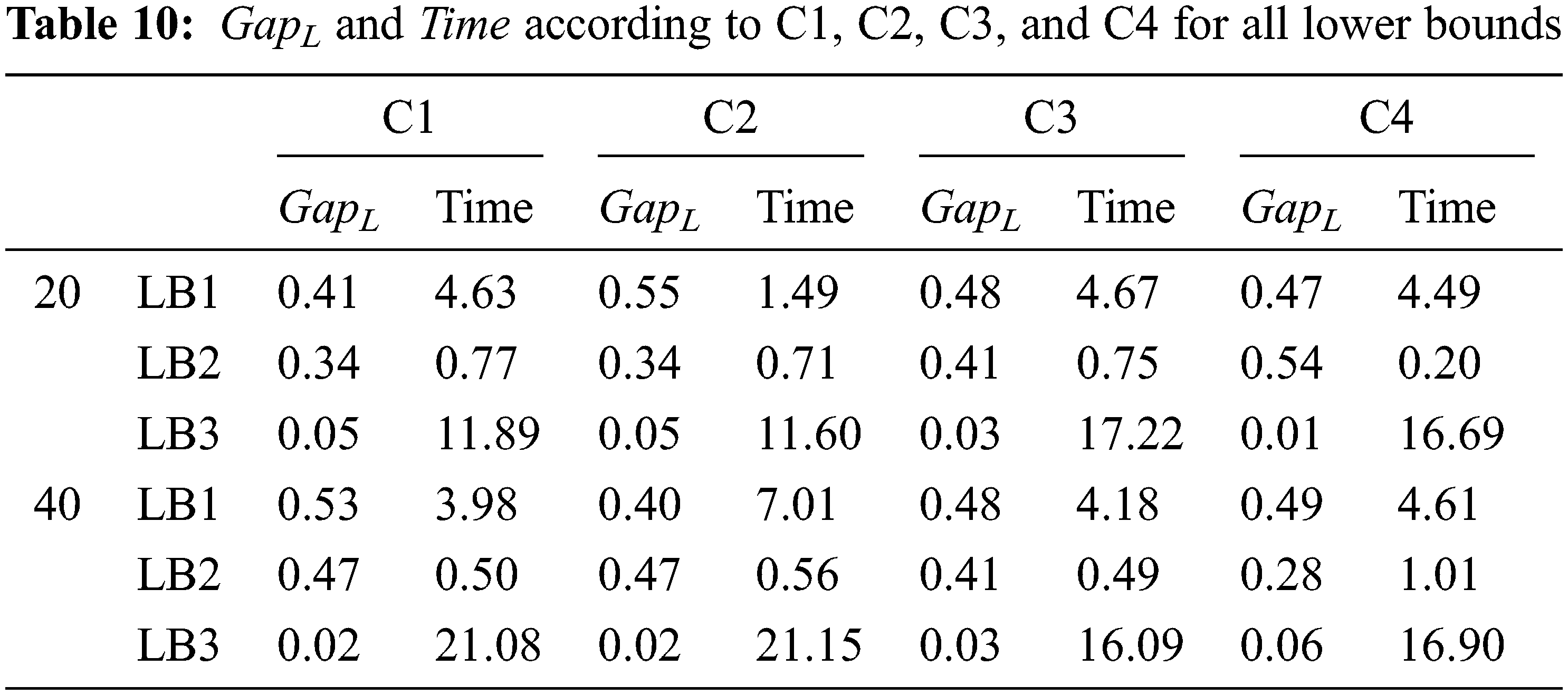
The variation of GapL and Time according to C1, C2, C3, and C4 for all lower bounds is illustrated in Tab. 10.
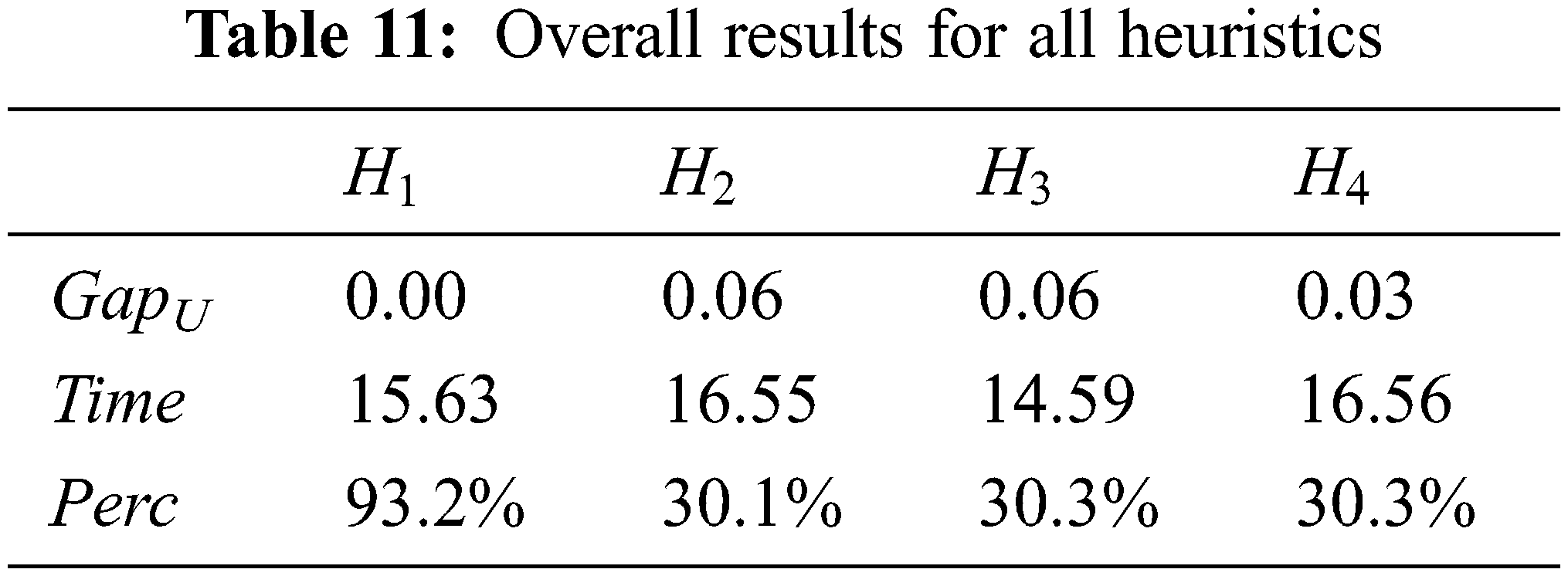
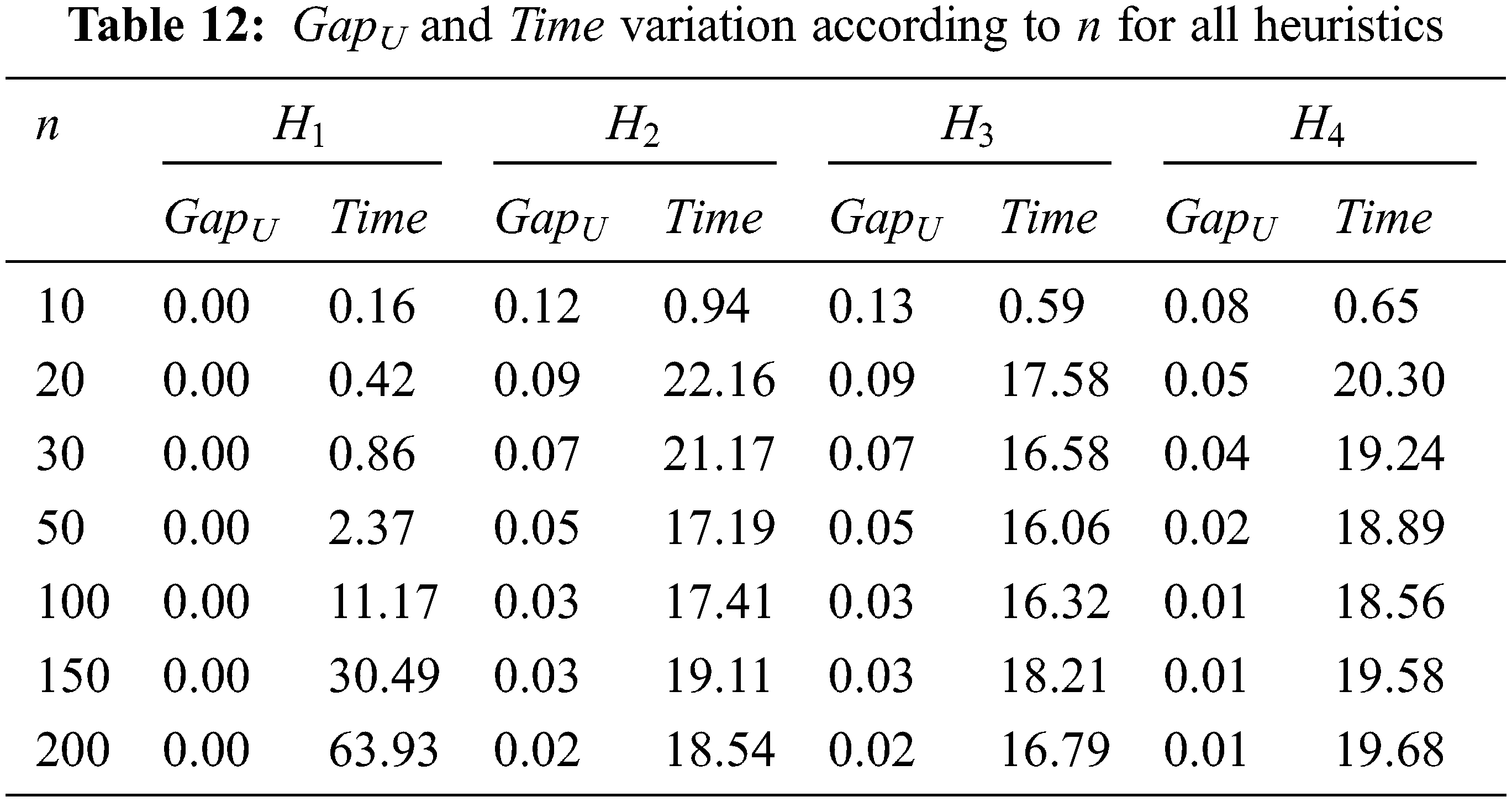
The assessment of the proposed heuristics is presented in Tabs. 11 and 12.
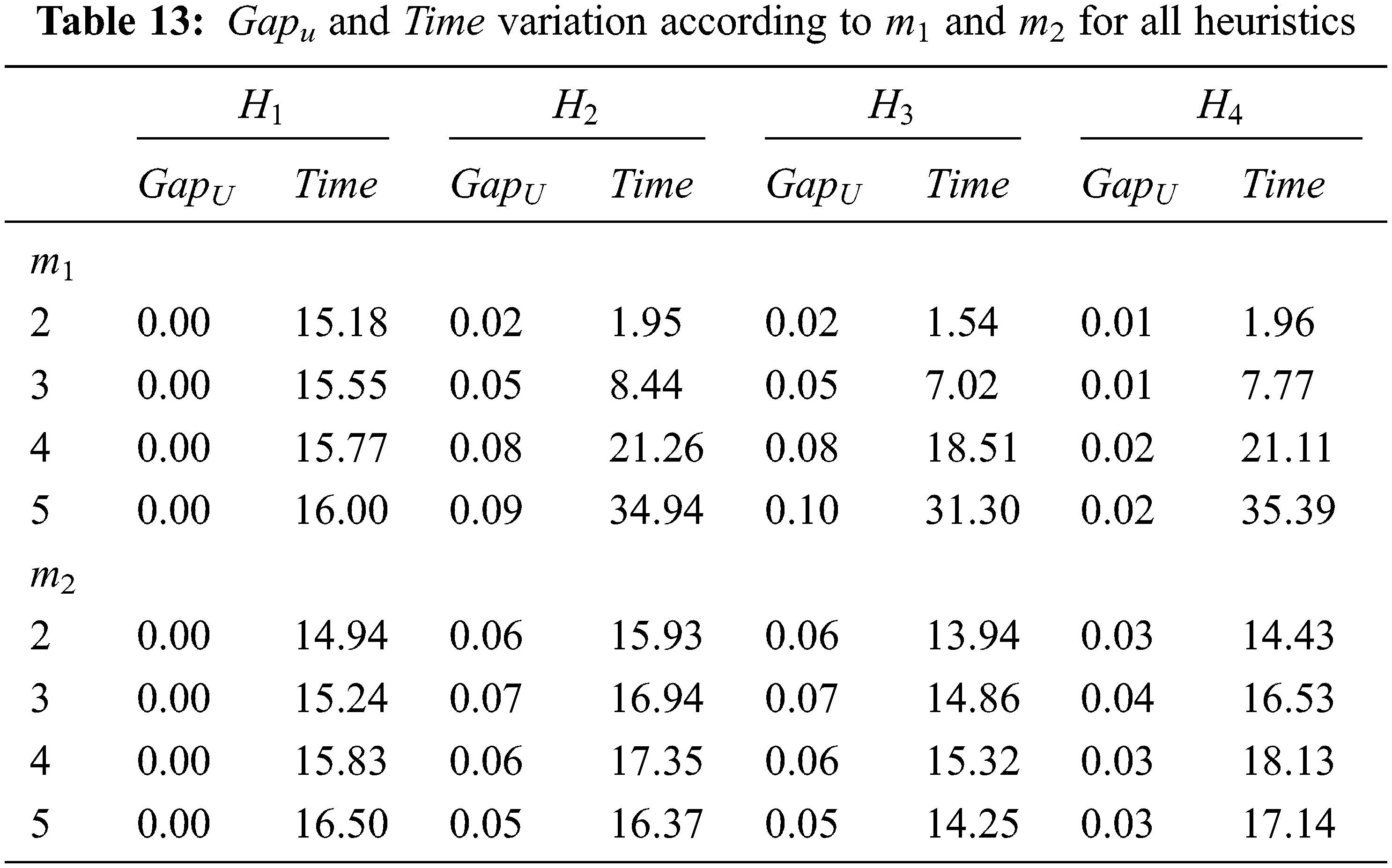
The behavior of GapU and Time according to m1 and m2 for all heuristics is presented in Tab. 13.
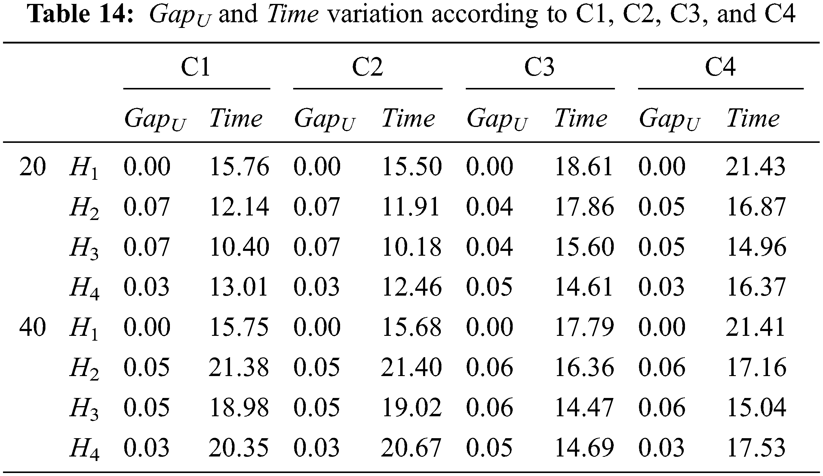
Tab. 14 presents the variation of GapU and Time for C1, C2, C3, and C4 for all heuristics. The maximum reaching time is 21.43 s. This running time is obtained for heuristic H1 when C4 = 20. However, the minimum reached time 10.18 s is obtained for H3 when C2 = 20.
This paper focuses on the two-stage hybrid flow shop problem under setup times. Several lower bounds and heuristics were developed. The exact resolution of the problem of the parallel machine is utilized in this paper to elaborate on lower bounds and heuristics. A genetic heuristic is developed for the metaheuristic. A comparison between lower bounds and heuristics is detailed to show the proposed algorithms’ performance in terms of gap and time. The genetic algorithm developed in this paper is the best heuristic comparing with the proposed others ones.
In future research work, the elaboration of exact solutions based on B&B algorithms could be considered. Indeed, the proposed heuristics and lower bounds in the paper can be used to elaborate such an exact algorithm. In addition, some other metaheuristics could be explored to detect the most appropriate ones to this scheduling problem.
Acknowledgement: The authors would like to thank the Deanship of Scientific Research at Majmaah University for supporting this work under Project Number No. 1439-19.
Funding Statement: The authors would like to thank the Deanship of Scientific Research at Majmaah University for supporting this work under Project Number No. 1439-19.
Conflicts of Interest: The authors declare that they have no conflicts of interest to report regarding the present study.
1. J. Alcaraz and C. Maroto, “A robust genetic algorithm for resource allocation in project scheduling,” Annals of Operations Research, vol. 102, pp. 83–109, 2001. [Google Scholar]
2. L. Shi, G. Guo and X. Song, “Multi-agent based dynamic scheduling optimization of the sustainable hybrid flow shop in a ubiquitous environment,” International Journal of Production Research, vol. 59, pp. 576–597, 2021. [Google Scholar]
3. W. Han, Q. Deng, G. Gong, L. Zhang and Q. Luo, “Multi-objective evolutionary algorithms with heuristic decoding for hybrid flow shop scheduling problem with worker constraint,” Expert Systems with Applications, vol. 168, pp. 114282, 2021. [Google Scholar]
4. W. Yankai, W. Shilong, L. Dong, S. Chunfeng and Y. Bo, “An improved multi-objective whale optimization algorithm for the hybrid flow shop scheduling problem considering device dynamic reconfiguration processes,” Expert Systems with Applications, vol. 174, pp. 114793, 2021. [Google Scholar]
5. M. Haouari, L. Hidri and A. Gharbi, “Optimal scheduling of a two-stage hybrid flow shop,” Mathematical Methods of Operations Research, vol. 64, pp. 107–124, 2006. [Google Scholar]
6. L. Hidri, S. Elkosantini and M. M. Mabkhot, “Exact and heuristic procedures for the two-center hybrid flow shop scheduling problem with transportation times,” IEEE Access, vol. 6, pp. 21788–21801, 2018. [Google Scholar]
7. H. Allaoui and A. Artiba, “Scheduling two-stage hybrid flow shop with availability constraints,” Computers & Operations Research, vol. 33, pp. 1399–1419, 2006. [Google Scholar]
8. S. Wang and M. Liu, “A genetic algorithm for two-stage no-wait hybrid flow shop scheduling problem,” Computers & Operations Research, vol. 40, pp. 1064–1075, 2013. [Google Scholar]
9. S. Wang, X. Wang and L. Yu, “Two-stage no-wait hybrid flow-shop scheduling with sequence-dependent setup times,” International Journal of Systems Science: Operations & Logistics, vol. 7, pp. 291–307, 2020. [Google Scholar]
10. Y. Tan, L. Mönch and J. W. Fowler, “A hybrid scheduling approach for a two-stage flexible flow shop with batch processing machines,” Journal of Scheduling, vol. 21, pp. 209–226, 2018. [Google Scholar]
11. J. Yang, “Minimizing total completion time in two-stage hybrid flow shop with dedicated machines,” Computers & Operations Research, vol. 38, pp. 1045–1053, 2011. [Google Scholar]
12. S. Wang and M. Liu, “A heuristic method for two-stage hybrid flow shop with dedicated machines,” Computers & Operations Research, vol. 40, pp. 438–450, 2013. [Google Scholar]
13. S. Wang, X. Wang, F. Chu and J. Yu, “An energy-efficient two-stage hybrid flow shop scheduling problem in a glass production,” International Journal of Production Research, vol. 58, pp. 2283–2314, 2020. [Google Scholar]
14. B. Fan, W. Yang and Z. Zhang, “Solving the two-stage hybrid flow shop scheduling problem based on mutant firefly algorithm,” Journal of Ambient Intelligence and Humanized Computing, vol. 10, pp. 979–990, 2019. [Google Scholar]
15. Y. Li, X. Li, L. Gao, B. Zhang, Q. K. Pan et al., “A discrete artificial bee colony algorithm for distributed hybrid flowshop scheduling problem with sequence-dependent setup times,” International Journal of Production Research, vol. 59, pp. 3880–3899, 2021. [Google Scholar]
16. H. Mirsanei, M. Zandieh, M. J. Moayed and M. R. Khabbazi, “A simulated annealing algorithm approach to hybrid flow shop scheduling with sequence-dependent setup times,” Journal of Intelligent Manufacturing, vol. 22, pp. 965–978, 2011. [Google Scholar]
17. H. T. Lin and C. J. Liao, “A case study in a two-stage hybrid flow shop with setup time and dedicated machines,” International Journal of Production Economics, vol. 86, pp. 133–143, 2003. [Google Scholar]
18. M. Hekmatfar, S. F. Ghomi and B. Karimi, “Two stage reentrant hybrid flow shop with setup times and the criterion of minimizing makespan,” Applied Soft Computing, vol. 11, pp. 4530–4539, 2011. [Google Scholar]
19. G. C. Lee, J. M. Hong and S. H. Choi, “Efficient heuristic algorithm for scheduling two-stage hybrid flowshop with sequence-dependent setup times,” Mathematical Problems in Engineering, vol. 2015, pp. 1–10, 2015. [Google Scholar]
20. S. Wang and M. Liu, “Two-stage hybrid flow shop scheduling with preventive maintenance using multi-objective tabu search method,” International Journal of Production Research, vol. 52, pp. 1495–1508, 2014. [Google Scholar]
21. R. L. Graham, E. L. Lawler, J. K. Lenstra and A. R. Kan, “Optimization and approximation in deterministic sequencing and scheduling: A survey,” Annals of Discrete Mathematics, vol. 5, pp. 287–326, 1979. [Google Scholar]
22. A. Gharbi and M. Haouari, “Minimizing makespan on parallel machines subject to release dates and delivery times,” Journal of Scheduling, vol. 5, pp. 329–355, 2002. [Google Scholar]
23. J. H. Holland, “Genetic algorithms and adaptation,” in Adaptive Control of Ill-Defined Systems, Springer: Boston, MA, vol. 16, pp. 317–333, 1984. [Google Scholar]
 | This work is licensed under a Creative Commons Attribution 4.0 International License, which permits unrestricted use, distribution, and reproduction in any medium, provided the original work is properly cited. |