DOI:10.32604/csse.2023.024154
| Computer Systems Science & Engineering DOI:10.32604/csse.2023.024154 | |
| Article |
Optimal Artificial Intelligence Based Automated Skin Lesion Detection and Classification Model
1Faculty of Engineering and the Built Environment, Department of Electrical and Electronics Engineering Technology, University of Johannesburg, Johannesburg, 2006, South Africa
2Center for Artificial Intelligence and Research (CAIR), Chennai Institute of Technology, Chennai, 600069, India
3Al-Nahrain Nanorenewable Energy Research Center, Al-Nahrain University, Baghdad, 64074, Iraq
*Corresponding Author: R. Surendran. Email: dr.surendran.cse@gmail.com
Received: 06 October 2021; Accepted: 17 November 2021
Abstract: Skin lesions have become a critical illness worldwide, and the earlier identification of skin lesions using dermoscopic images can raise the survival rate. Classification of the skin lesion from those dermoscopic images will be a tedious task. The accuracy of the classification of skin lesions is improved by the use of deep learning models. Recently, convolutional neural networks (CNN) have been established in this domain, and their techniques are extremely established for feature extraction, leading to enhanced classification. With this motivation, this study focuses on the design of artificial intelligence (AI) based solutions, particularly deep learning (DL) algorithms, to distinguish malignant skin lesions from benign lesions in dermoscopic images. This study presents an automated skin lesion detection and classification technique utilizing optimized stacked sparse autoencoder (OSSAE) based feature extractor with backpropagation neural network (BPNN), named the OSSAE-BPNN technique. The proposed technique contains a multi-level thresholding based segmentation technique for detecting the affected lesion region. In addition, the OSSAE based feature extractor and BPNN based classifier are employed for skin lesion diagnosis. Moreover, the parameter tuning of the SSAE model is carried out by the use of sea gull optimization (SGO) algorithm. To showcase the enhanced outcomes of the OSSAE-BPNN model, a comprehensive experimental analysis is performed on the benchmark dataset. The experimental findings demonstrated that the OSSAE-BPNN approach outperformed other current strategies in terms of several assessment metrics.
Keywords: Deep learning; dermoscopic images; intelligent models; machine learning; skin lesion
Skin cancer has become the deadliest disease among humans. Every year, around 2 to 3 million non-melanoma cases are identified worldwide, with approximately 130,000 melanoma cases [1]. Melanoma is a kind of cancer that affects the skin. It isn’t the most common, but it is the most dangerous since it spreads quickly. Doctors have recommended that the better method for detecting malignant skin lesions of all kinds is earlier recognition. The rate of survival rises to approximately 99% for a period of 5 years when diseases are detected in the earlier stage [2]. Dermoscopic or epilumine scence microscopy (ELM) is a medical procedure that aids a clinician in determining if a skin lesion is cancerous or benign. This method makes use of a dermatoscope, that is an instrument with an amplification lens and a light source for improving the view of medical patterns such as globs, ramifications, veils, hues, and pigmented networks [3]. Following that, the image processing approaches were developed, and computer aided detection (CAD) approaches and systems in the segmentation and classification of a pigmented skin lesion (PSL), allowing patient to be diagnosed at an earlier stages of the disease without undergoing painful/shocking medical processes [4]. Skin cancer segmentation is an important step for all classification methods. A current study of automatic skin cancer segmentation algorithms was established in [5,6]. Precise segmentation could benefit the accuracy of succeeding lesion classification. Described an unsupervised method for skin cancer segmentation termed Independent histogram pursuit (IHP). Using mean shift, presented many strategies for segmenting skin lesions in dermoscopic images [7,8]. Created an automated skin lesions segmentation approach using a hybrid threshold algorithm and the best color channel [9]. In current, studies, Delaunary triangulation was applied to extract binary masks of the skin cancer region that are not needed at all training stages [10]. A new deformable method utilizing a recently determined ending condition and speed function for skin cancer segmentation, i.e., stronger toward noise and yield flexible and effective segmentation performances was introduced [11]. We proposed a deep learning method which is a fully convolutional residual network (FCRN) for skin cancer segmentation in dermoscopy images [12]. This study designs a novel skin lesion diagnosis model using an optimized stacked sparse autoencoder (OSSAE) with a backpropagation neural network (BPNN), named the OSSAE-BPNN model. The proposed technique contains a multi-level thresholding based segmentation (MLTBS) technique for detecting the affected lesion region where the optimal threshold values are chosen using the jellyfish search algorithm (JSA). Besides, OSSAE based feature extractor and a BPNN based classifier are employed for skin lesion diagnosis. In addition, the seagull optimization algorithm (SGO) is used for tuning the parameters of SSAE model. Experiments on the benchmark dataset were carried out to illustrate the increased performance of the OSSAE-BPNN model.
Through one of the discriminative deep features, Khan et al. [13] developed a completely automated technique for multiclass skin cancer segmentation and classification. To begin, LCcHIV improves the input images. Then, saliency is calculated by a new deep saliency segmentation approach that utilizes a custom CNN of 10 layers. The produced heat maps are transformed to binary images through thresholding function. Then, the segmented colour images are utilized to extract features using a deep pertained convolutional neural network (CNN) method. To evade the curse of dimensionality, they implemented an IMFO method for selecting the most discriminative features. The KELM classifiers integrate the resultant characteristics with an MMCA and classify them. Based on a DL architecture, Khan et al. offer a completely automated CAD method. Before being sent to the MASK-RCNN for cancer segmentation, the original dermoscopic images are first preprocessed using the decorrelation formulation method [14]. The segmented images are segmented using the DenseNet deep technique, which is then displayed using an entropy-controlled LS-SVM.
Rodrigues et al. presented the usage of DL and TL in an IoT method for assisting physicians in the diagnosis of typical nevi, melanoma, and common skin lesions [15]. This work exploits CNN as a resources extractor. The CNN method consists of Inception, VGG, Inception-ResNet, ResNet, MobileNet, Xception, NASNet, and DenseNet. For the classifications of injury, the Bayes, SVM, RF, MLP, and KNN are utilized. Sikkandar et al. Introduced a novel segmentation based classification technique for skin cancer diagnoses with the combination of ANFC and GrabCut models [16]. The presented technique includes 4 main stages: segmentation, preprocessing, classification, and feature extraction. First, the preprocessing phase is performed by an inpainting and top hat filter method. Next, the Grabcut approach is utilized for segmenting the preprocessed image. Then, the feature extraction procedure is performed using the DL-based inception method. Finally, an ANFC system is used to classify dermoscopic images into various types. Goyal et al. [17] presented the fully automatic ensemble DL method for achieving higher sensitivity and specificity in cancer edge segmentation. Two different classifiers such as feature-based, neural network are combined and a new method is proposed by El-Khatib et al. [18]. Depending on the projected accuracy, each approach (classifier) provides a specific weight to the final decision scheme, aiding the scheme in reaching the best conclusion feasible. First, they made an NN that could distinguish melanoma from benign nevus. Next, they proposed 3 approaches on the basis of CNN. The CNN is pretrained by huge ImageNet and Place365 databases. NasNet-Large, GoogleLeNet, and ResNet-101, are utilized in the enumeration order. Krishnaraj et al. [19] proposed a high-performance and low-cost data augmentation approach that consists of 2 successive phases of network search and augmentation search. In the network search phase, the DCNN is fine-tuned using the entire training set to select the method with the maximum BACC.
Fig. 1 shows the procedure for running the recommended the OSSAE-BPNN model. The suggested OSSAE-BPNN model is designed to detect and characterize skin lesions automatically using dermoscopic images. The OSSAE-BPNN model includes image preprocessing, MLTBS-based segmentation, OSSAE-based feature extraction, SGO-based parameter optimization, and BPNN-based classification. In the next sections, we’ll look at how these modules operate in detail.
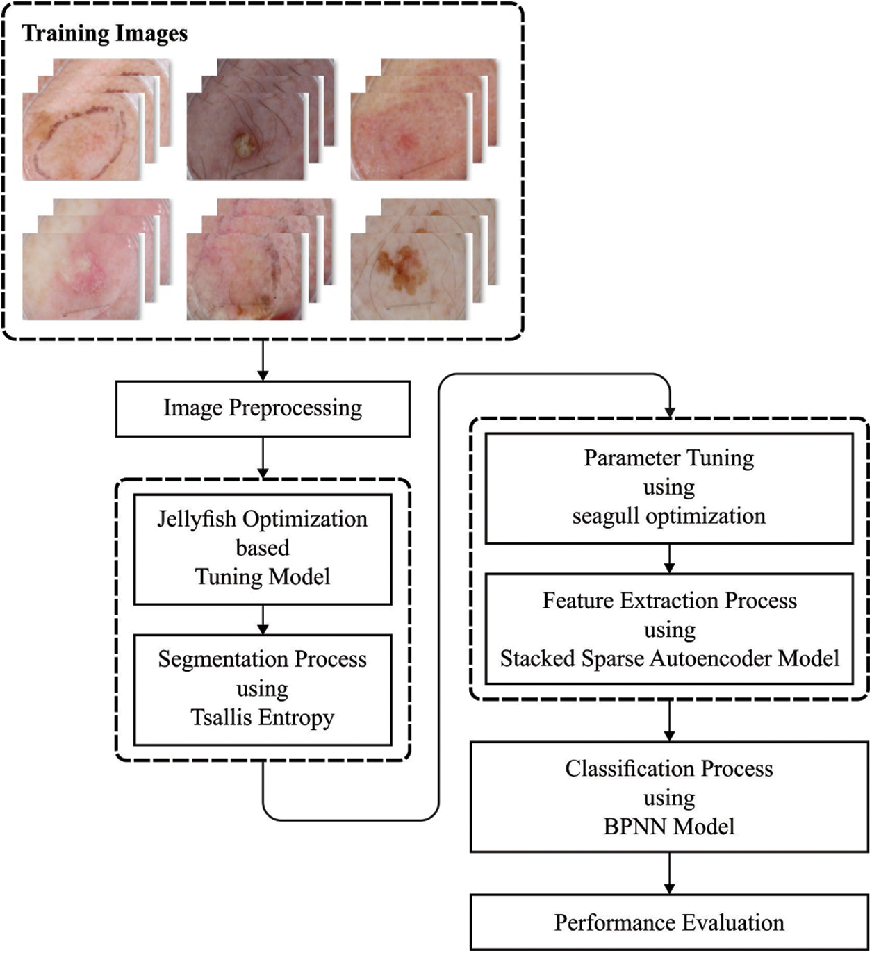
Figure 1: Overall process of OSSAE-BPNN model
This method finds the location of images and removes the hair. First, the images are resized to a uniform size, and a class labeling process takes place. These data comprise values for intermediate coordinate points, such as the height (h) and width (w) of bounding boxes where object class descriptions must be established, make up this data. In addition, the hair removal process takes place on the dermoscopic images by the use of the DullRazor [20] technique to precisely detect and remove hairs. To achieve this, primarily, the position of the hair is detected using the grayscale morphological closing function. In addition, the hair position is ensured by determining the length and thickness of the determined shapes, and pixels are substituted by the use of a bilinear interpolation approach.
The MTLBS approach is used to determine the afflicted lesion areas using the preprocessed images. The MTLBS technique incorporates the design of Tsallis entropy and the AFS based threshold selection. The entropy is associated with chaos measures within a scheme. Shannon first examines the entropy for evaluating ambiguity based on the scheme’s data content [21–24]. When a physical scheme is split into two statistically free subsystems A & B, Shannon defined that the entropy value may be expressed as follows:
According to the Shannon concept, a nonextensive entropy theory was developed by Tsallis is given as follows:
whereas T represents the scheme potential, q indicates the entropic index, and pi signifies the likelihood of all states i. Generally, the Tsallis entropy Sq would meet the Shannon entropy if q → 1. The entropy value could be stated as follows:
Tsallis entropy could be considered to detect an optimum threshold of an image. Consider an image using L gray levels in the range
In which
In the multilevel threshold procedure, it is essential to determine the optimum threshold value T that maximizes the objective function f(T). In the current study, (f(T)) maximization was executed by the AFS approach. In recent times, a novel metaheuristic approach depending on the behavior of jellyfish, the JSA (an optimizer), was developed to solve optimization problems. Jellyfish search for food using ocean movement and current within a swarm on time. In the initialization stage, the solution is effectively dispersed within the search space of the problems for covering all the spaces. The method does not descend terminally to a local minimum and speeds up convergence toward the optimum solution. They calculated various chaotic maps and aimed to optimize population initialization within the search space. The logistic map was optimum. Earlier in optimization, the initialized solution is related based on the quality, and is appropriately selected as the food position
where
where r3 implies an arbitrary number in the range of zero & one, and γ > 0 specifies the movement length near the present position [22–24]. Ub and Lb represent the search boundary of the problem and, hence, are the upper bound and lower bound respectively.
j refers to the index of a solution elected arbitrarily. To model the tradeoffs among the ocean current and the active and passive movements, a predetermined constant c0 and the time control function are arithmetically shown in Eq. (12) is utilized to produce the time control method.
where t denotes the current estimation, tmax represents maximal calculation, and r indicates an arbitrary value in the range of zero & one. If c(t) ≥ c0, the solution is upgraded in the ocean. If the arbitrary number r4 in the range of zero & one is higher than (1 − c(t)), then current solutions are upgraded by passive movement; otherwise, active movement is applied.
The segmented images are fed into the OSSAE model to generate a collection of feature vectors during the feature extraction phase. In all networks, the SSAE technique is illustrated using a two-level network with five hidden layers. In the initial level network, the input layer X is mapped to a hidden layer h3 (named the low level hidden feature). Next, h3 is mapped back to the recreated layer, Xrec. In the 2nd level network, the hidden feature vectors h3 are converted to the input parameter for acquiring h6 (high level hidden feature). In SSAE, the feature learning procedure trails a sequence of functions such as convolution, denoising, activation, pooling, and BN [25–27]. A summary of the operation is defined as follows:
To attain the representative and robust learned features of the flame image, a denoising AE learning approach is utilized by including distinct noises with the input signal [25–28]. However, distinct kinds of corruption procedures could be taken into account, such as mask noise, Gaussian, and salt-and-pepper noise. In this work, white Gaussian noise is taken into account, e.g., the corrupted form Xn is attained by a set corruption ratio to the input X, as follows:
Let
Convolution process can be a practical solution for extracting features. Using a convolutional layer, a feature map could be produced by sliding multiple filters on the entire input sequence. Every filter scans the input neuron with fixed stride and size and generates a feature map that can be considered the input of the following convolution layer. A ReLU is utilized as the activation function of hidden neuron γ, as follows:
The ReLU is an unsaturated piecewise linear function, i.e., quicker than saturated nonlinear functions such as TanH and sigmoid. Particularly, the sigmoid function is utilized in the 3rd decoders to ensure that the intensity range of the recreated layer Xrec is reliable with the input layer X, as follows:
Pooling and upsampling can be performed to reduce the network parameters. In this work,P(r × r + t) represents the pooling layer that condenses the feature map by electing a maximal value with a r × r conversion kernel and a phase of t. The pooling process is beneficial for improving the translation in-variance, as follows:
where
At the same time, the parameters involved in the SSAE model can greatly influence the overall classification performance which needs to be properly tuned by the use of the SGO technique. The SGO algorithm is designed based on the nature of the shell game. Few assumptions are made in the design of the SGO algorithm.
• Here, a person is treated as the operator of the game
• A ball and 3 shells are presented to the operator
• Every individual player gets two chances to tell the proper shell.
Here, a collection of N persons is treated as the game player. In Eq. (17), place ‘d’ of player ‘I’ can be presented by
where, Xi is an arbitrary value for the problem parameter. Depending upon the value of Xi, the value of the fitness function is determined for the players. Once the fitness value is determined, the operator of the game can choose 3 shells where a shell is linked to the location of the optimal player and the rest of them are chosen in an arbitrary way.
where Xbest denotes the location of the minimum or maximum, fitness and
where AIi is the accuracy and intelligence of player i. Here, the player is prepared to presume the ball. Provided a game with 3 shells and the player has two opportunities and there exist 2 states of deductions for every player. First, the deduction might be accurate and the place of the ball can be determined. Next, the layer identifies the ball only in the second chance. Finally, the player fails to identify the location of the ball. The guess vector defined Gv is based on Eq. (20) for every player.
The possibility of selecting a state to select the shell can be performed using Eq. (21).
where rg1 denotes the chance of right deduction at the primary election and rg2 signifies the chance of right deduction at the next time. Finally, the Xi vector is considered the place of every member of the population, and is upgraded using Eqs. (22)–(25).
where ri represents an arbitrary value that exists in the range of [0 1],
The BPNN model is used to derive the appropriate class labels for the applied dermoscopic images during the image classification process. BPNN is an ANN that is divided into three layers: output, input, and hidden. It is a type of multilayer forward NN. Its major feature is the reverse transmissions of error and signal. Backward and forward procedures were continued untill the variances among the output and training data met the training accuracy (the maximum value i.e., satisfactory for the mean errors among real and training data). The regular BPNN utilizes a gradient descent approach, and the network weight is altered contrariwise and the gradient of the efficiency function. Hence, the anticipated values approach the real values. Fig. 2 represents the framework of BPNN.
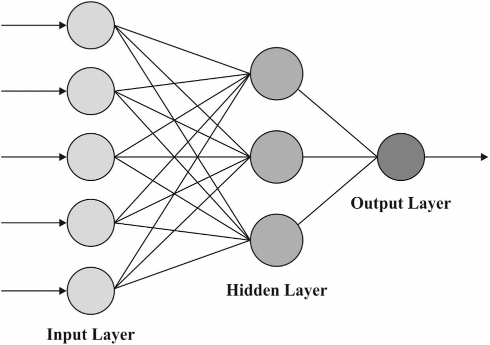
Figure 2: BPNN framework
To interconnect the input database from Layer n − 1, and output data to Layer n + 1, the formula for an individual neuron in Layer n can be represented by the following equation:
where
The output function can be represented by the following equation:
In this section, performance validation is done by experimenting the performance of OSSAE-EPNN techniques used on the applied datasets. It contains a set of images under seven distinct classes namely Angioma (0), Nevus (1), Lentigo NOS (2), Solar Lentigo (3), Melanoma (4), Seborrheic Keratosis (5), and Basal Cell Carcinoma (6). Few of the sample test images are illustrated in Fig. 3.
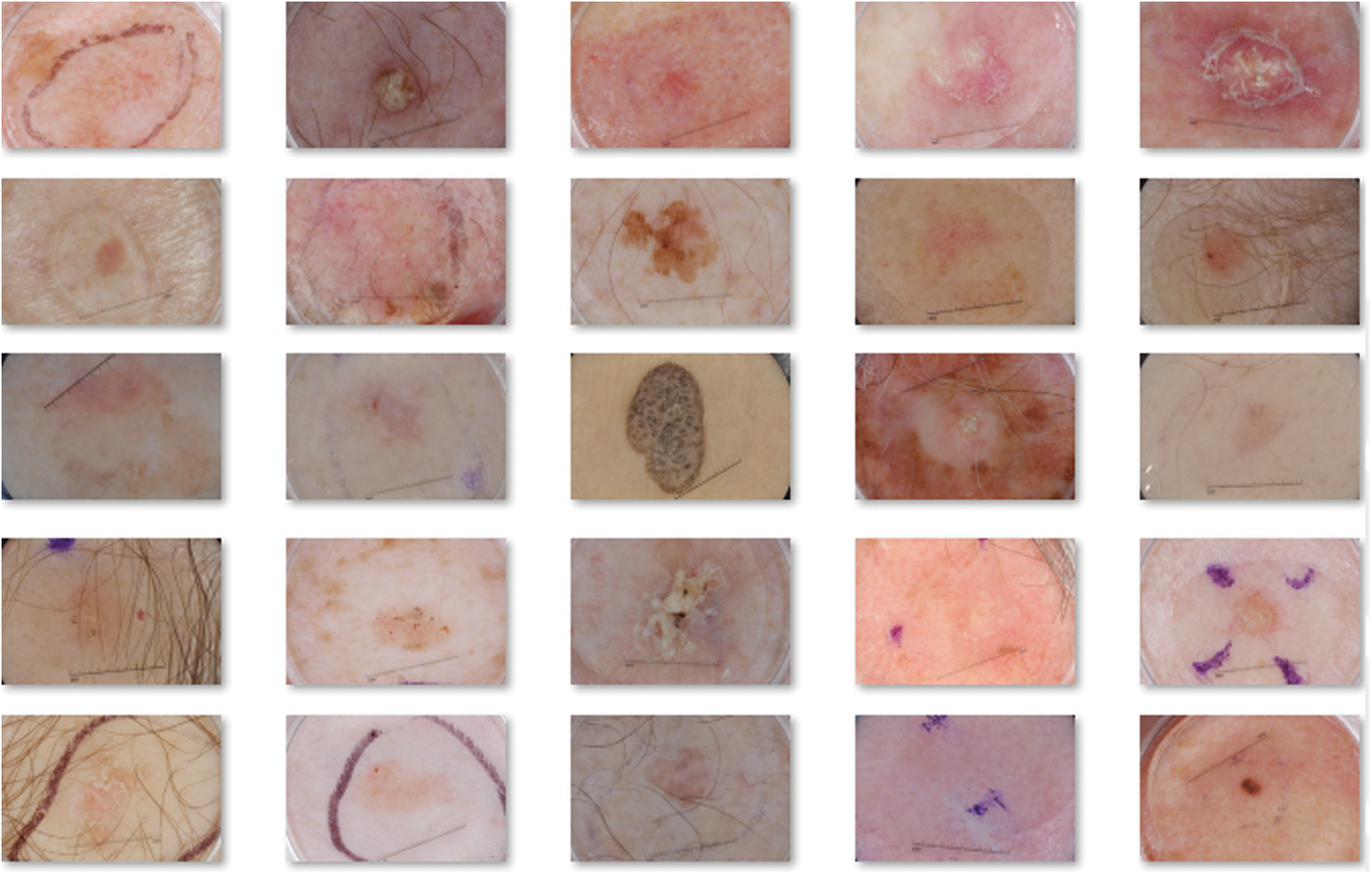
Figure 3: Sample images
Fig. 4 visualizes the sample preprocessed outcome offered by the OSSAE-BPNN technique. It shows that the input image is properly preprocessed and the hair in the segmented region is removed clearly.
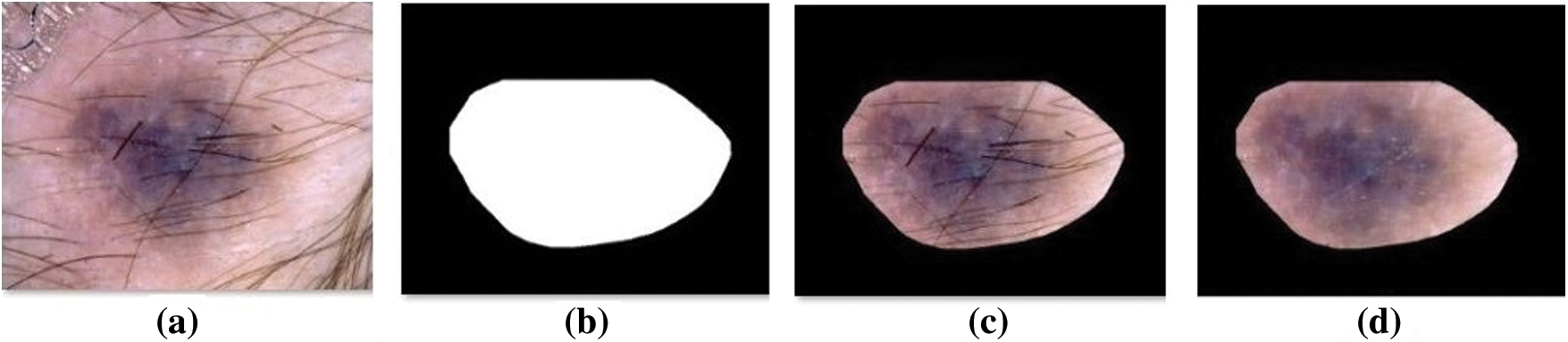
Figure 4: Sample preprocessed images a) Original image b) Ground truth c) Segmented d) Hair removed
During the training phase, a confusion matrix which is created by the OSSAE-EPNN method on the dataset is described in the Fig. 5. This figure shows that the OSSAE-BPNN technique categorized 13 images into class 0, 38 images into class 1, 41 images into class 2, 55 images into class 3, 52 images into class 4, 46 images into class 5, and 32 images into class 6.A confusion matrix produced by the OSSAE-BPNN method on the applied dataset in the testing phase is exhibited in Fig. 6. The figure outperformed that the OSSAE-BPNN manner categorized 13 images into class 0, 36 images into class 1, 35 images into class 2, 58 images into class 3, 45 images into class 4, 43 images into class 5, and 29 images into class 6. A detailed classification results of the OSSAE-BPNN technique during training and testing phases are given in Tab. 1. The OSSAE-BPNN approach categorized the images with a maximum average accuracy (0.962), the sensitivity (0.853), specificity (0.978), precision of 0.854, and F-score of 0.849 after evaluating the data from the training phase. Similarly, the OSSAE-BPNN method categorized the images with a maximum average accuracy (0.947), the sensitivity (0.796), specificity (0.969), precision (0.806), and F-score (0.796) throughout the testing phase.
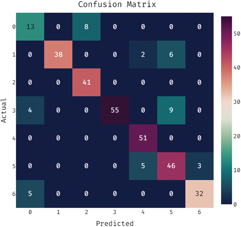
Figure 5: Confusion matrix analysis of OSSAE-BPNN under training phase
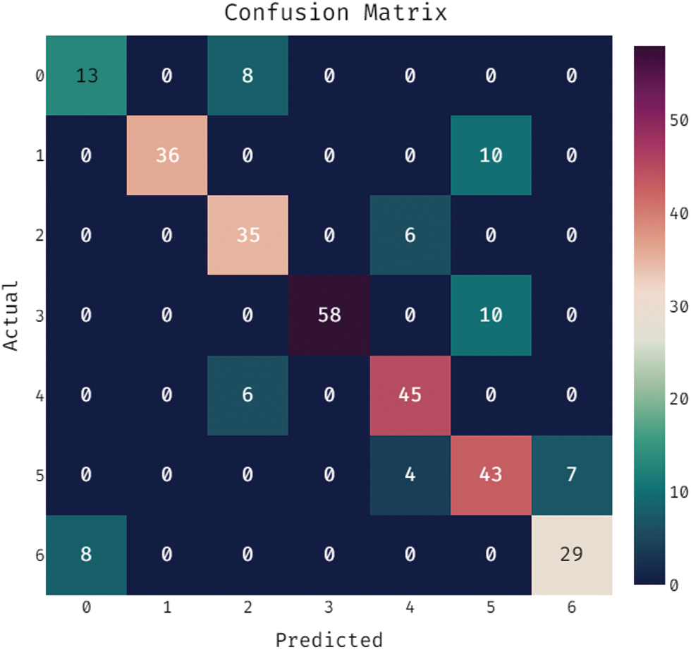
Figure 6: Confusion matrix analysis of OSSAE-BPNN under testing phase
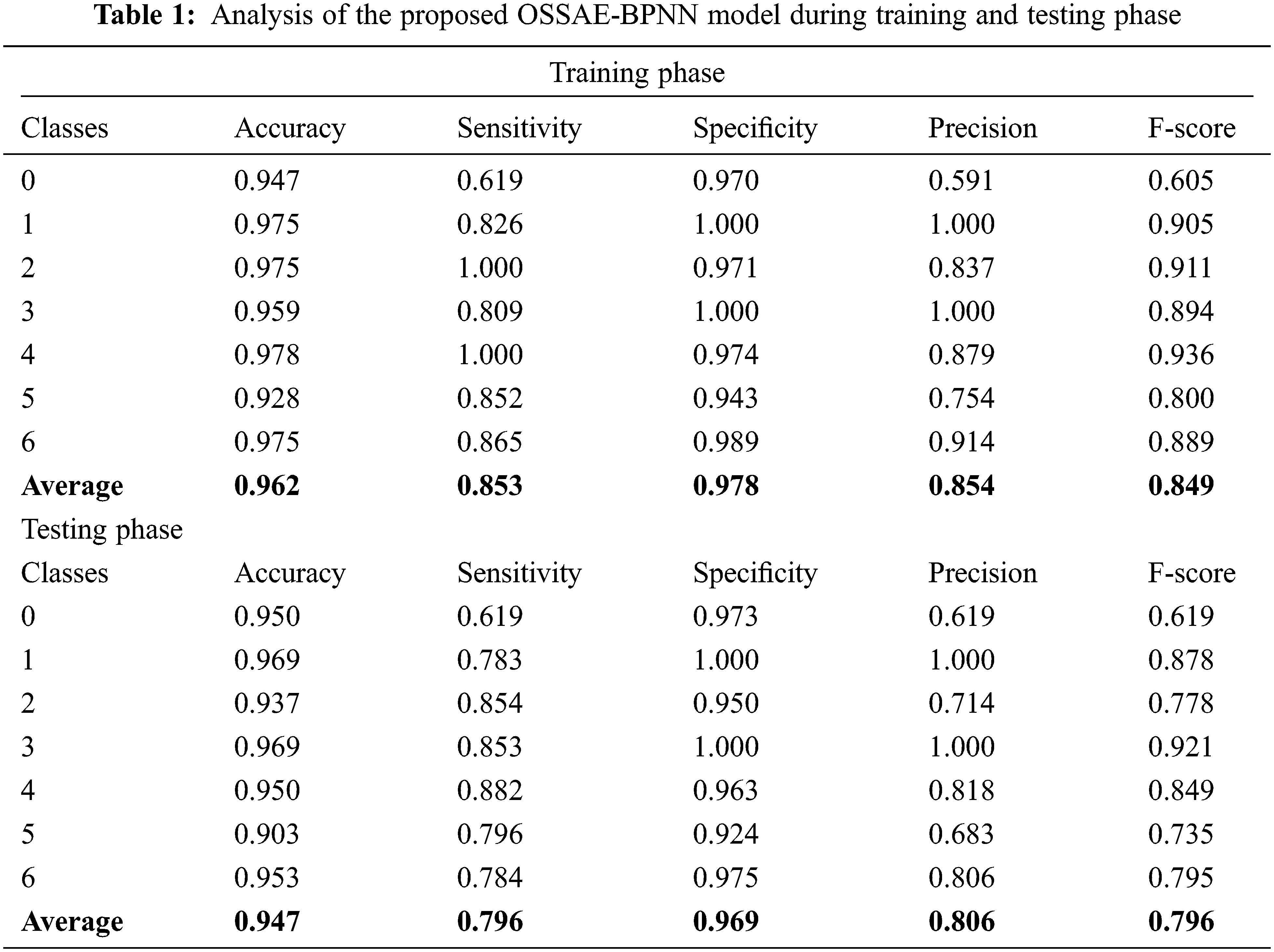
Fig. 7 ROC analysis of the OSSAE-BPNN technique the training phase. Figure showcs that the OSSAE-BPNN technique has resulted in a higher ROC of 98.7379.

Figure 7: ROC analysis of OSSAE-BPNN under training phase
Fig. 8 showcases the ROC analysis of the OSSAE-BPNN algorithm under the testing phase. The figure outperformed that the OSSAE-BPNN methodology has resulted in a maximum ROC of 98.7152. Finally, a comparison study of the OSSAE-BPNN technique with existing techniques takes place in Tab. 2. Fig. 9 showcases the training and testing accuracy values of the OSSAE-BPNN technique with existing techniques. The figure shows that VGG-16 attained ineffective outcomes with training accuracy pf 0.886 and testing accuracy of 0.849, respectively. Additionally, the VGG-19, Xception, R.NET, and D.NET techniques have obtained slightly enhanced training and testing accuracy values. Next, moderate training and testing accuracy has been achieved using the Inception-V3 and MN-v1 methods. Furthermore, with training and testing accuracies of 0.924 and 0.897, respectively. The MN-v2 method has attempted to provide competitive outcomes. However, the proposed OSSAE-BPNN technique has resulted in a superior outcome with training and testing accuracies of 0.962 and 0.947 respectively. From the detailed result analysis, it is demonstrated that the proposed OSSAE-BPNN technique has been found to be an appropriate tool for effective skin lesion diagnosis.
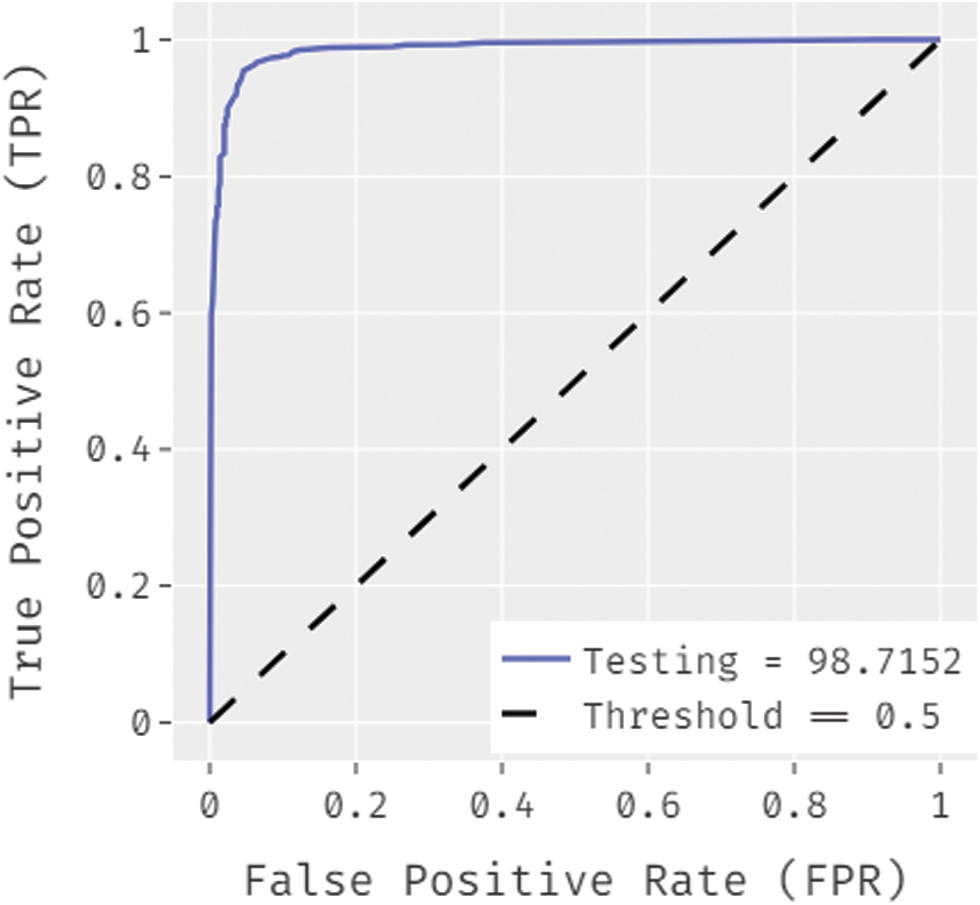
Figure 8: ROC analysis of OSSAE-BPNN under ROC-testing phase
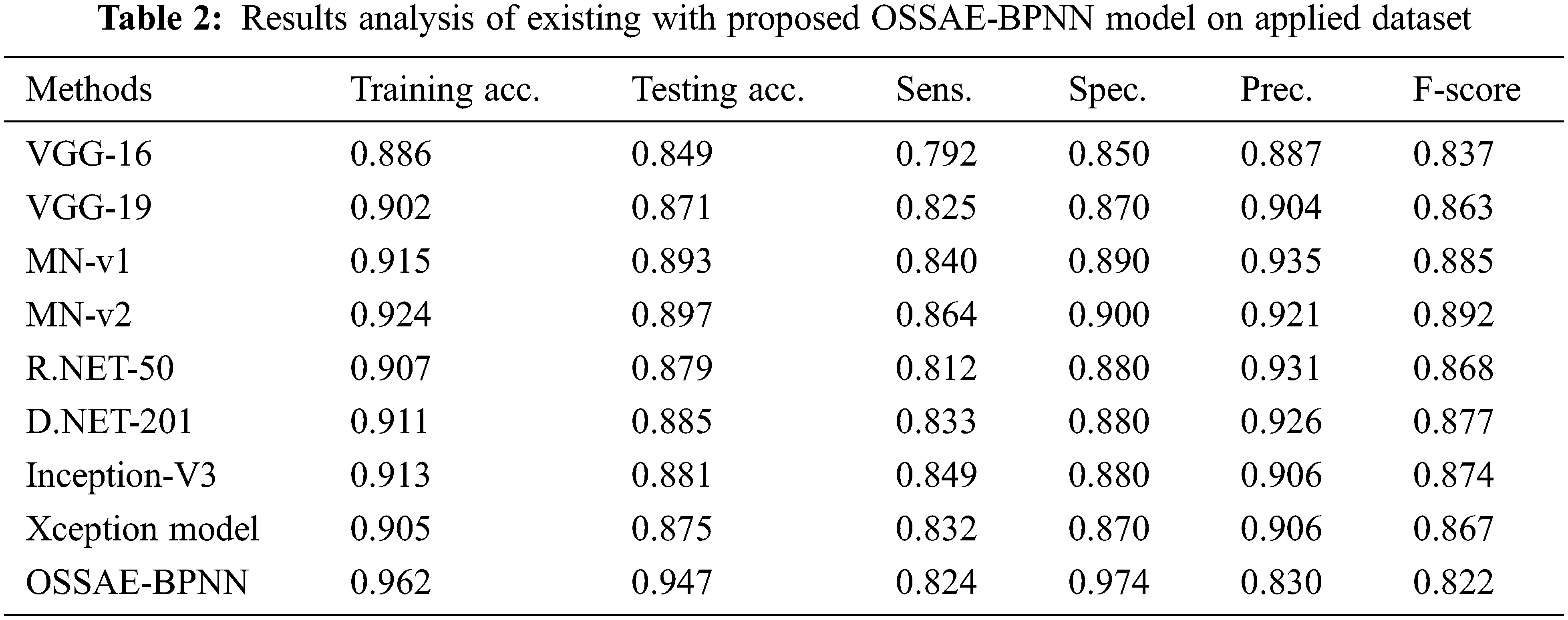
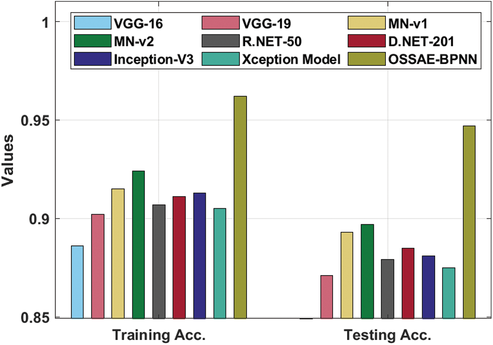
Figure 9: Training and testing accuracy analysis of OSSAE-BPNN model
Fig. 10 illustrates the sensitivity and specificity values of the OSSAE-BPNN approach with recent algorithms. The figure shows that VGG-16 attained ineffective outcomes with the lowest sensitivity and specificity of 0.792 and 0.850, respectively. Additionally, the R.NET, VGG-19, Xception, and D.NET methods have reached somewhat improved sensitivity and specificity values. Followed by, the MN-v1 and Inception-V3 approaches resulted in moderate sensitivity and specificity. On continuing with, a MN-v2 algorithm has tried to outperform competitive outcomes with the sensitivity and specificity of 0.864 and 0.900, respectively. Eventually, the presented OSSAE-BPNN methodology has resulted in an improved outcome with the sensitivity and specificity of 0.824 and 0.974, respectively. From the brief outcome analysis, it can be demonstrated that the projected OSSAE-BPNN technique has been found to be a suitable tool for effectual skin lesion diagnosis.
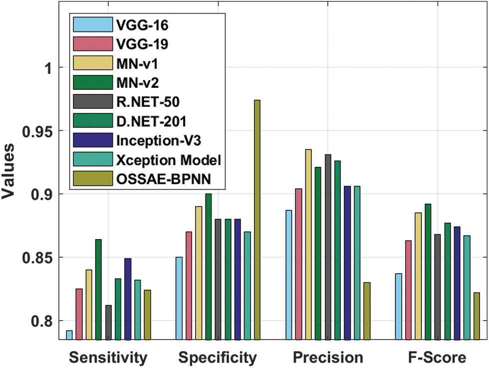
Figure 10: Comparative analysis of OSSAE-BPNN model with different measures
This study designed a novel OSSAE-BPNN model to distinguish malignant skin lesions in dermoscopic images. which shows the differences among various malignant as well as benign skin lesions in dermoscopic images. The suggested OSSAE-BPNN model uses dermoscopic images to automatically detect and categorize skin lesions. Image preprocessing, SGO-based parameter optimization, OSSAE-based feature extraction, MLTBS-based segmentation, and BPNN-based classification are all part of the OSSAE-BPNN model. The proposed model involves MLTBS based segmentation with the inclusion of the Otsu thresholding with the JSA technique to effectually determine the affected lesion regions. Experiments on the benchmark dataset were carried out to illustrate the increased performance of the OSSAE-BPNN model. The testing findings demonstrated that the OSSAE-BPNN approach outperformed other current strategies in terms of several assessment metrics. Advanced DL structures might be utilized in the future for skin lesion segmentation methods to improve diagnosis results.
Acknowledgement: The authors would like to thank University of Johannesburg, Chennai Institute of Technology, Al-Nahrain University for providing us with various resources and an unconditional support for carrying out this study.
Funding Statement: This work is funded by University Research Committee fund URC-UJ2019, awarded to Kingsley A. Ogudo.
Conflicts of Interest: The authors declare that they have no conflicts of interest to report regarding the present study.
1. J. A. A. Damian, V. Ponomaryov, S. Sadovnychiy and H. C. Fernandez, “Melanoma and nevus skin lesion classification using handcraft and deep learning feature fusion via mutual information measures,” Entropy, vol. 22, no. 4, pp. 484–503, 2020. [Google Scholar]
2. A. Baldi, M. Quartulli, R. Murace, E. Dragonetti, M. Manganaro et al., “Automated dermoscopy image analysis of pigmented skin lesions,” Cancers, vol. 2, no. 2, pp. 262–273, 2010. [Google Scholar]
3. Y. Li and L. Shen, “Skin lesion analysis toward melanoma detection using deep learning network,” Sensors, vol. 18, no. 556, pp. 1–18, 2018. [Google Scholar]
4. K. M. Hosny and M. A. Kassem, “Foaud, M.M. classification of skin lesions using transfer learning and augmentation with alex-net,” PLoS ONE, vol. 14, no. e0217293, pp. 1–16, 2019. [Google Scholar]
5. Y. Li and L. Shen, “Skin lesion analysis toward melanoma detection using deep learning network,” Sensors (Basel), vol. 18, no. 2, pp. 556–774, 2018. [Google Scholar]
6. M. E. Celebi, Q. Wen, H. Iyatomi, K. Shimizu, H. Zhou et al., “A state-of-the-art survey on lesion border detection in dermoscopy images,” in Dermoscopy Image Analysis, 1st ed, California, USA: O Reilly, pp. 98–104, 2015. [Google Scholar]
7. D. D. Gomez, C. Butakoff, B. K. Ersboll and W. Stoecker, “Independent histogram pursuit for segmentation of skin lesions,” IEEE Transactions on Biomedical Engineering, vol. 55, pp. 157–161, 2008. [Google Scholar]
8. G. Suryanarayana, K. Chandran, O. I. Khalaf, Y. Alotaibi, A. Alsufyani et al., “Accurate magnetic resonance image super-resolution using deep networks and Gaussian filtering in the stationary wavelet domain,” IEEE Access, vol. 9, pp. 71406–71417, 2021. [Google Scholar]
9. R. Garnavi, M. Aldeen, M. E. Celebi, G. Varigos and S. Finch, “Border detection in dermoscopy images using hybrid thresholding on optimized color channels,” Computerized Medical Imaging and Graphics, vol. 35, pp. 105–115, 2011. [Google Scholar]
10. A. Pennisi, D. D. Bloisi, D. Nardi, A. R. Giampetruzzi, C. Mondino et al., “Skin lesion image segmentation using delaunay triangulation for melanoma detection,” Computerized Medical Imaging and Graphics, vol. 52, pp. 89–103, 2016. [Google Scholar]
11. Z. Ma and J. Tavares, “A novel approach to segment skin lesions in dermoscopic images based on a deformable model,” IEEE Journal Biomedical Health Informatics, vol. 20, pp. 615–623, 2017. [Google Scholar]
12. L. Yu, H. Chen, Q. Dou, J. Qin and P. A. Heng, “Automated melanoma recognition in dermoscopy images via very deep residual networks,” IEEE Transactions on Medical Imaging, vol. 36, pp. 994–1004, 2017. [Google Scholar]
13. M. A. Khan, M. Sharif, T. Akram, R. Damasevicius and R. Maskeliunas, “Skin lesion segmentation and multiclass classification using deep learning features and improved moth flame optimization,” Diagnostics, vol. 11, no. 5, pp. 811–830, 2021. [Google Scholar]
14. M. A. Khan, T. Akram, Y. D. Zhang and M. Sharif, “Attributes based skin lesion detection and recognition: A mask RCNN and transfer learning-based deep learning framework,” Pattern Recognition Letters, vol. 143, pp. 58–66, 2021. [Google Scholar]
15. D. D. A. Rodrigues, R. F. Ivo, S. C. Satapathy, S. Wang, J. Hemanth et al., “A new approach for classification skin lesion based on transfer learning, deep learning, and IoT system,” Pattern Recognition Letters, vol. 136, pp. 8–15, 2020. [Google Scholar]
16. M. Y. Sikkandar, B. A. Alrasheadi, N. B. Prakash, G. R. Hemalakshmi, A. Mohanarathinam et al., “Deep learning based an automated skin lesion segmentation and intelligent classification model,” Journal of Ambient Intelligence and Humanized Computing, vol. 12, no. 3, pp. 3245–3255, 2021. [Google Scholar]
17. M. Goyal, A. Oakley, P. Bansal, D. Dancey and M. H. Yap, “Skin lesion segmentation in dermoscopic images with ensemble deep learning methods,” IEEE Access, vol. 8, pp. 4171–4181, 2019. [Google Scholar]
18. H. El-Khatib, D. Popescu and L. Ichim, “Deep learning–based methods for automatic diagnosis of skin lesions,” Sensors, vol. 20, no. 6, pp. 1753–1768, 2020. [Google Scholar]
19. N. Krishnaraj, M. Elhoseny, E. L. Lydia, K. Shankar and O. A. L. Dabbas, “An efficient radix trie-based semantic visual indexing model for large-scale image retrieval in cloud environment,” Software: Practice and Experience, vol. 51, no. 3, pp. 489–502, 2021. [Google Scholar]
20. O. I. Khalaf, C. A. T. Romero, A. A. J. Pazhani and G. Vinuja, “VLSI implementation of a high-performance nonlinear image scaling algorithm,” Journal of Healthcare Engineering, vol. 2021, no. 6297856, pp. 1–10, 2021. [Google Scholar]
21. T. Lee, V. Ng, R. Gallagher, A. Coldman and D. McLean, “A software approach to hair removal from images,” Computers in Biology and Medicine, vol. 27, no. 6, pp. 533–543, 1997. [Google Scholar]
22. V. Rajinikanth, S. C. Satapathy, S. L. Fernandes and S. Nachiappan, “Entropy based segmentation of tumor from brain MR images–a study with teaching learning based optimization,” Pattern Recognition Letters, vol. 94, pp. 87–95, 2017. [Google Scholar]
23. M. A. Basset, R. Mohamed, M. Abouhawwash, R. K. Chakrabortty, M. J. Ryan et al., “An improved jellyfish algorithm for multilevel thresholding of magnetic resonance brain image segmentations,” Computers, Materials & Continua, vol. 68, no. 3, pp. 2961–2977, 2021. [Google Scholar]
24. N. A. Khan, O. I. Khalaf, C. A. T. Romero, M. Sulaiman and M. A. Bakar, “Application of euler neural networks with soft computing paradigm to solve nonlinear problems arising in heat transfer,” Entropy, vol. 23, pp. 1053–1064, 2021. [Google Scholar]
25. G. Li, F. Liu, A. Sharma, O. I. Khalaf, Y. Alotaibi et al., “Research on the natural language recognition method based on cluster analysis using neural network,” Mathematical Problems in Engineering, vol. 2021, no. 9982305, pp. 1–13, 2021. [Google Scholar]
26. Y. Q. Feng, Y. Z. Liu, X. Wang, Z. X. He, T. C. Hung et al., “Performance prediction and optimization of an organic rankine cycle (ORC) for waste heat recovery using back propagation neural network,” Energy Conversion and Management, vol. 226, pp. 113552, 2020. [Google Scholar]
27. S. Dalal and O. I. Khalaf, “Prediction of occupation stress by implementing convolutional neural network techniques,” Journal of Cases on Information Technology, vol. 23, no. 3, pp. 27–42, 2021. [Google Scholar]
28. M. Krichen, S. Mechti, R. Alroobaea, E. Said, P. Singh et al., “A formal testing model for operating room control system using internet of things,” Computers, Materials & Continua, vol. 66, no. 3, pp. 2997–3011, 2021. [Google Scholar]
 | This work is licensed under a Creative Commons Attribution 4.0 International License, which permits unrestricted use, distribution, and reproduction in any medium, provided the original work is properly cited. |