Computer Systems Science & Engineering DOI:10.32604/csse.2023.024217
Article

Covid-19 Forecasting with Deep Learning-based Half-binomial Distribution Cat Swarm Optimization

P. Renukadevi1,* and A. Rajiv Kannan2

1Department of Computer Science and Engineering, Paavai Engineering College, Namakkal, 637018, Tamil Nadu, India
2Department of Computer Science and Engineering, K.S.R. College of Engineering, Tiruchengode, Namakkal, 637215, Tamil Nadu, India
*Corresponding Author: P. Renukadevi. Email: pgrenu@gmail.com
Received: 09 October 2021; Accepted: 10 January 2022

Abstract: About 170 nations have been affected by the COvid VIrus Disease-19 (COVID-19) epidemic. On governing bodies across the globe, a lot of stress is created by COVID-19 as there is a continuous rise in patient count testing positive, and they feel challenging to tackle this situation. Most researchers concentrate on COVID-19 data analysis using the machine learning paradigm in these situations. In the previous works, Long Short-Term Memory (LSTM) was used to predict future COVID-19 cases. According to LSTM network data, the outbreak is expected to finish by June 2020. However, there is a chance of an over-fitting problem in LSTM and true positive; it may not produce the required results. The COVID-19 dataset has lower accuracy and a higher error rate in the existing system. The proposed method has been introduced to overcome the above-mentioned issues. For COVID-19 prediction, a Linear Decreasing Inertia Weight-based Cat Swarm Optimization with Half Binomial Distribution based Convolutional Neural Network (LDIWCSO-HBDCNN) approach is presented. In this suggested research study, the COVID-19 predicting dataset is employed as an input, and the min-max normalization approach is employed to normalize it. Optimum features are selected using Linear Decreasing Inertia Weight-based Cat Swarm Optimization (LDIWCSO) algorithm, enhancing the accuracy of classification. The Cat Swarm Optimization (CSO) algorithm’s convergence is enhanced using inertia weight in the LDIWCSO algorithm. It is used to select the essential features using the best fitness function values. For a specified time across India, death and confirmed cases are predicted using the Half Binomial Distribution based Convolutional Neural Network (HBDCNN) technique based on selected features. As demonstrated by empirical observations, the proposed system produces significant performance in terms of f-measure, recall, precision, and accuracy.

Keywords: Binomial distribution; min-max normalization; Cat Swarm Optimization (CSO); COVID-19 forecasting

1  Introduction

The world is dealing with the Unique Corona Virus (COVID-19) epidemic, which reached in December 2019 in Wuhan, China [1–3]. From December 2019 onwards, most countries worldwide have experienced an increase in COVID-19 cases. Around 353 373 deaths and 5 596 550 cases were reported worldwide, as mentioned in the World Health Organization report dated May 29, 2020. People at old age, low immunity, and medical issues primarily related to lungs are highly prone to COVID 19 disease. Breathing problems, cold, and cough similar to flu are the significant symptoms of COVID-19 [4]. There are no effective therapeutics, drugs, and licensed vaccines for COVID-19 or Severe Acute Respiratory Syndrome Corona Virus 2 (SARS-CoV-2). For controlling the COVID-19 outbreak, various strategies are adopted by different countries because of the absence of pharmaceutical interventions. The most common method used is nationwide lockdown [5].

The local Wuhan government first used it on January 23, 2020, when the city was temporarily closed down to prohibit all public travel and quickly followed by many other cities in Hubei province.

Preserving social isolation is the best technique to reduce human-to-human broadcast of coronavirus disease in the absence of medications or specific antiviral for COVID-19, and therefore stringent lockdowns, quarantines, and curfews have also been incorporated by other nations.

The first coronavirus occurrence in India was reported on January 30, 2020, in the Thrissur region of Kerala, whenever a student returned from Wuhan, China’s sprawling capital [6]. The Government of India enforced a complete national lockdown throughout the country on March 25, 2020, for 21 days and one day "Janata Curfew" on March 22, 2020, to fight the coronavirus SARS-CoV-2 epidemic in India. The government of India has prolonged the lockdown owing to massive coronavirus disease dissemination. Preventive steps for Covid19 are to protect oneself by constantly washing one’s hands, not rubbing one’s lips, nose and ears, and keeping social distance from other people (1 meter or 3 feet). Regularly, confirmed cases have risen in all countries. The transmission of such a virus is risky and needs stricter measures and plans already placed in place in many cities.

In hospitals, accurate COVID-19 cases forecasting is necessary, and it enhances the management strategies in managing infected patients in an optimum manner. Deep learning and machine learning have recently been considered as a leading study subject across a wide variety of applications, particularly in business and academia [7,8].

For predicting COVID-19 future, four algorithms, namely, Support Vector Machine (SVM), Exponential Smoothing (ES), Least Absolute Shrinkage and Selection Operator (LASSO) regression, and linear regression, are applied in [9], and these algorithms are supervised machine learning algorithms. In the prediction of death count, recoveries count, contaminated cases count, other models are outperformed by ES as shown. ES includes information in previous data prediction while managing time-series data. As a result, ES is a powerful tool. In more than 100 countries, for forecasting new and cumulative death and confirmed COVID 19 cases under different intervention conditions in real-time, a Modified Auto-Encoder (MAE) is developed in [10], and it is an Artificial Intelligence (AI) based technique. This technique does not provide satisfactory results concerning prediction accuracy and computation complexity.

In the latest days, advances in computer vision applications such as segmentation, identification, and object detection have indeed been made breakthroughs to the use of deep learning methods in general and convolutional neural networks (CNNs) in particular. Deep learning algorithms are very effective in automating feature-representation learning and removing the time-consuming effort of handcrafted feature engineering. Deep learning and convolutional neural networks (CNNs) use a hierarchical layer of feature representation to replicate the human visual cortex system in terms of structure and functioning. This multi-layer feature representation methodology allowed CNNs to automatically nalyse different image features, allowing them to outperform feature approaches.

The main concern of this research work is the classification of COVID-19. Several methodologies have been introduced, but the COVID-19 identification accuracy is not significant. The existing approaches have drawbacks with error rates and inaccurate COVID dataset classification results. The LDIWCSO-HBDCNN method is proposed to improve the overall system performance. The main contribution of this research is data normalization, feature selection, and classification. The proposed technique for the given COVID dataset is employed to produce more accurate findings using effective algorithms.

The remainder of the article is organized as shown: The prediction model from past research is presented in Section 2. The proposed technique is presented in Section 3. The findings and performance analysis are presented in Section 4. Lastly, Section 5 concludes the study and discusses future research possibilities.

2  Literature Review

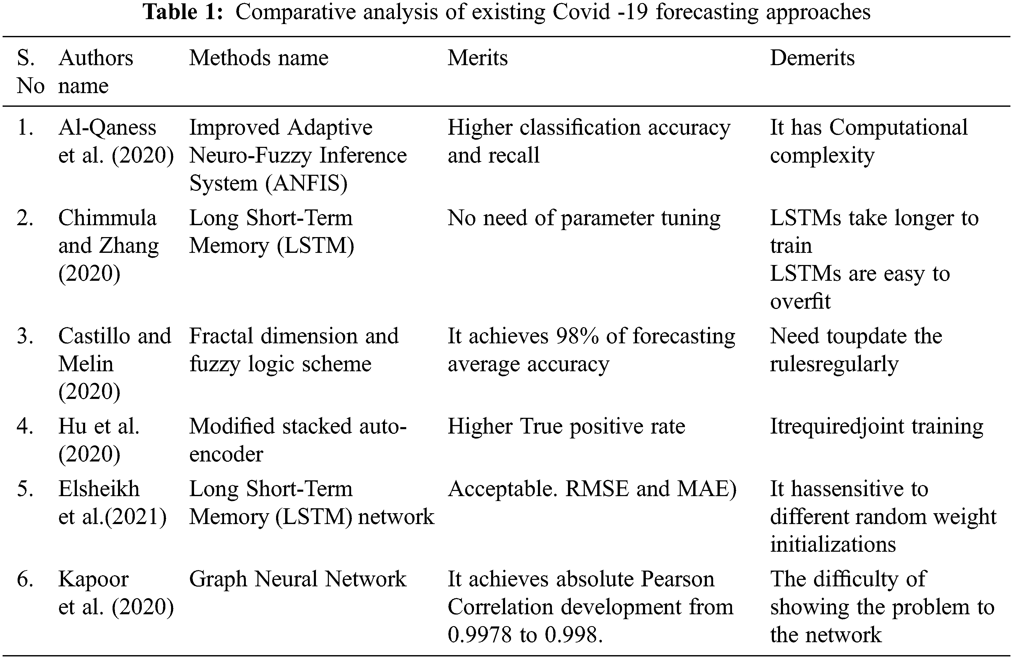
An enhanced Adaptive Neuro-Fuzzy Inference System (ANFIS) has been introduced by Al-Qaness et al. [11]. This system used the Salp Swarm Algorithm (SSA) and enhanced Flower Pollination Algorithm (FPA). For improving FPA, SSA is applied in general as FPA may get trapped with local optimum. The primary objective of this FPASSA-ANFIS model is to improve the ANFIS performance via the computation of ANFIS parameters by using FPASSA.

The official COVID 19 outbreak data given by WHO concerning confirmed cases in the upcoming ten days is used to evaluate this model. The FPASSA-ANFIS model shows significant performance based on the computing time, coefficient of determination (R2), RMSRE, MAPE, better performance.

Chimmula et al. [12] used a Long Short-Term Memory (LSTM) network to forecast the present COVID-19 epidemic in Canada and throughout the world. The University of Johns Hopkins and the Canadian Health Authority gathered COVID-19 data for this research and delivered several verified cases by March 31, 2020. The data collection includes the number of fatalities and restored patients every day.

Wavelet transformation is employed to maintain the time-frequency components while simultaneously reducing the random noise in the database. The Long Short-Term Memory (LSTM) networks are then utilized to assess future COVID-19 instances. The COVID-19 data is divided into a training set (80%) for training the models and a test set (20%) for testing the model’s results. The system provided a greater prediction accuracy.

Castillo et al. [13] created a hybrid technique that combines the fractal dimension with fuzzy logic to enable effective and accurate COVID-19 time series prediction. The data sets from ten countries worldwide are utilized to build the fuzzy model using time series in a specified timeframe. Following that, further periods were employed to test the viability of the proposed approach for the predicted values of the ten countries. Given the difficulties of the COVID issue, the average forecast accuracy is 98% that may be considered good.

Hu et al. [14] developed the Artificial Intelligence (AI)-inspired algorithms for real-time Covid-19 prediction to assess the size, period, and end time of Covid-19 throughout China. A modified stacked auto-encoder was employed to represent epidemic transmission dynamics. This approach was employed to predict observed Covid-19 instances in China in real time. The database was obtained by WHO between January 11 and February 27, 2020.

The provinces/cities for transmission architecture investigation were organized using latent variables from the auto-encoder and clustering methods. Utilizing multiple-step predicting, the computed average errors of 6-step, 7-step, 8-step, 9-step, and 10-step predictions were 1.64%, 2.27%, 2.14%, 2.08%, and 0.73%, correspondingly.

Elsheikh et al. [15] suggested a deep learning-based prediction system for COVID-19 pandemic in Saudi Arabia. The Long Short-Term Memory (LSTM) network forecasts the total reported cases, total retrieved cases, and total deaths in Saudi Arabia in this investigation as a complete DL model. The model was educated based on the official records. The ideal settings of the model’s parameters that optimize predicting precision have been identified.Seven statistical assessment parameters, namely Coefficient of Residual Mass (CRM), coefficient of variation (COV), Overall Index (OI), Efficiency Coefficient (EC), MAE,coefficient of determination (R2) and RMSE are employed to forecast the model’s accuracy.

Kapoor et al. [16] developed a novel forecasting technique for COVID-19 instance detection employing Graph Neural Networks and mobility data. The proposed method is based on a single large-scale Spatio-temporal graph with nodes representing regional human mobility, spatial edges representing inter-regional connection based on human mobility, and temporal edges representing node attributes across time. This technique is tested on the COVID-19 database at the county level in the United States, demonstrating that the graph neural network’s rich geographical and temporal data allows the model to learn complicated dynamics. Tab. 1 shows the comparative analysis of existing Covid -19 forecasting approaches. Around 6% minimization in Root Mean Squared Log Error (RMSLE) and improvement in absolute Pearson Correlation to 0.998 from 0.9978can be achieved as shown in results when compared with baseline models.

3  Proposed Methodology

For forecasting COVID-19, Linear Decreasing Inertia Weight based Cat Swarm Optimization with Half Binomial Distribution based Convolutional Neural Network (LDIWCSO-HBDCNN) technique is proposed in this research work. Fig. 1 shows the proposed work’s flow diagram.

Figure 1: Suggested system flow diagram

3.1 Input

The input corresponds to the COVID-19 forecasting dataset.

From https://www.kaggle.com/davidbnn92/weather-data-for-covid19-data-analysis, this dataset is collected. Information like fog, temperature, fatalities, confirmed cases, date, long, lat, region, state, id are added in this dataset. The weather data is obtained from the National Oceanic and Atmospheric Administration & Global Surface summary of the Day (NOAA GSOD) dataset. Recent measurements are included using continuous updates.

3.2 Data Normalization Using Min-Max Normalization

A mathematical function converts the numerical values into new range values in the normalization process. The covid-19 dataset is normalized using min-max normalization in this proposed research work. Data are generally normalized using a standard technique called min-max normalization. From the dataset, within the specified maximum and minimum range, values are normalized, and using the following expression, every value is replaced.

v′=v−minAmaxA−minA(new_maxA−new_minA)+new_minA (1)

where,

A indicates Attribute data,

Min(A) is a minimum absolute value of A, Max(A) is a maximum absolute value of A

v′ indicates every entry’s new value in data

v indicates every entry’s old value in data

new_max(A) indicted maximum value of range, new_min(A) indicated min value of range (i.e, mandatory boundary value series)

3.3 Feature Selection Using Linear Decreasing Inertia Weight Based Cat Swarm Optimization (LDIWCSO) Algorithm

The Linear Decreasing Inertia Weight based Cat Swarm Optimization (LDIWCSO) algorithm selects normalized features. A new Cat Swarm Optimization algorithm has been developed according to the cat’s behavior. This algorithm has two search modes, Tracing Mode (TM) and Seeking Mode (SM). A cat’s capacity to keep aware of its environment when at rest is modelled in seeking mode. Tracing and catching the targets of cats is emulated in tracing mode. Optimization problems are solved using these modes.

Features are given as input in this proposed research work. Here, every feature is assigned with a fitness value, velocity, and position in a specified population. A point with respect to possible feature set represented by position. In a D-dimensional space, distance variance is represented using velocities. The solution set’s quality is represented using fitness value. Fitness function corresponds to classification accuracy n this proposed work.

Fitnessfunction=Max(Accuracy) (2)

Features are distributed to tracing or seeking mode randomly by CSO in every generation. Then altered every feature’s position. At last, the feature’s position with the highest accuracy value indicates the best feature. Fig. 2 shows Cat Swarm Optimization (CSO) system.

CSO Process

The cat’s percentage (features) distributed to tracing mode is represented using Mixture Ratio (MR). As much time is spent on testing by cats, the MR value will be minimal. Following outlines this process as

(1) Within a D-dimensional space, N features are initialized with velocities and positions.

(2) Features are distributed to tracing or seeking mode; features count in two modes defines MR.

(3) Every feature’s accuracy value is measured.

(4) In every iteration, they are searched based on the cat’s mode. The following subsection, describes the process involved in these two modes.

(5) If the terminal requirements are met, the algorithm is terminated; it returns to step (2) for the next cycle.

Seeking Mode

There are four operations in seeking mode; namely, Counts of Dimension to Change (CDC), Seeking Range of the selected Dimension (SRD), Self-Position Consideration (SPC), and Seeking Memory Pool (SMP). Seeking memory’s pool size is defined by SMP. For instance, the SMP value of 5 represents that every cat can store 5 result sets as candidates.

SPC is a Boolean value. One position within a memory retains the current solution set if SPC is true and not changed. Seeking range’s minimum and maximum values are defined by SRD. In the seeking process, dimensions count to be changed is represented using CDC. The steps of the seeking process are discussed below.

(1) Current feature position’s SMP copies are generated. One of these copies retains the current feature position if SPC is true and becomes a candidate immediately. Before becoming candidates, other features need to be changed. Otherwise, searching is performed by all SMP copies and its results in its position change.

(2) By altering CDC’s dimension percent, the position of every copy to be changed is changed randomly. The CDC’s dimensions percent is selected initially. The SRD percent’s current value is decreased or increased by changing every dimension chosen randomly. After changes are made, copies become a candidate.

(3) Every candidate’s fitness value is computed through the fitness function.

(4) The likelihood of each candidate being chosen is calculated. The chosen probability ( Pi ) equals one, and if all candidates have the same fitness value, else, using expression (3), Pi is computed. Range of i– lies between 0 and SMP; Pi gives candidates selection probability; Pi Overall fitness values maximum value is represented as FSmax , and minimum value is represented as FSmin ; ΦΣι gives candidates fitness value FSi

If the objective is to find a solution set having maximum fitness

Value, then FSb = FSmin ; else FSb = FSmax . As a result of this function’s probability computation, better candidates have a larger chance of getting chosen, and vice versa, as shown below:

Pi=|FSi−FSb|FSmax−FSmin (3)

(5) One candidate is selected randomly based on selected probability (Pi). The current feature is moved to this position after choosing the candidate.

Tracing Mode. Cats target tracing is represented using tracing mode. Here the same strategy is followed.

(1) Expression (4) is used for updating velocities.

(2) Current feature’s position is updated using expression(5) as mentioned below:

vk,dt+1=vk,dt+r1×c1×(xbest,dt−xk,dt) (4)

d = 1,2,..,D,

xk,dt+1=xk,dt+vk,dt (5)

where,

xk,dt and vk,dt are current feature k’s position and velocities at iteration t

xbest,dt gives the best solution set from featurek in population

c1 is constant

r1 is an arbitrary number that lies between 0 and 1

Linear Decreasing Inertia Weight based Cat Swarm Optimization (LDIWCSO) Algorithm

One of the most effective algorithms for computing the best global solution is conventional CSO. But, for producing an acceptable solution, CSO may consume a long time in rare cases. So, the algorithm’s convergence and performance may get affected by this. A new parameter, inertia weight (w), is added in the expression used for updating positions to solve this issue. An algorithm’s tracing mode, a new velocity update form is used. A Linear Decreasing Inertia Weight factor is introduced in this work and it has a linear decrement to wmin from wmax with respect to iteration’s increment and they indicates final and initial values. Reformed expressions are mentioned below.

vk,dt+1=w∗vk,dt+r1×c1×(xbest,dt−xk,dt) (6)

W=wmax−wmax−wminitermax×k (7)

vk,dt+1=(wmax−wmax−wminitermax×k)∗vk,dt+r1×c1×(xbest,dt−xk,dt) (8)

where,

w gives inertia weight

wmax represents maximum weight value

wmin representsminimum weight value

itermax indicates maximum iteration

k is a Constant

Figure 2: Flow diagram of the cat swarm optimization (CSO) method

3.4 Classification Using Half Binomial Distribution Based Convolutional Neural Network (HBDCNN)

This research work uses Half Binomial Distribution based Convolutional Neural Network (HBDCNN) for classification. The CNN [17,18] is a robust deep learning algorithm. This network shows excellent efficiency in different areas, especially in computer vision. There are three types of layers in CNN: fully connected, sub-sampling, and convolution layers [19,20]. A convolutional neural network’s (CNN) typical structure is depicted in Fig. 3. The following section explains every layer type.

Figure 3: Convolutional neural network

Convolution Layer

selected features are given as input in this proposed work. With a kernel (filter), these input features are convolved in this convolution layer. The n output features are generated using this convolution result between kernel and input feature. In general, the filter is a convolution matrix kernel. The feature map with i*i size refers to output features that convolve input and kernel.

Multiple convolutional layers are present in the CNN architecture. The feature vector is given as an input to the subsequent convolutional layers, and it produces the same at the output. In every convolution layer, there is filter bunch n. The input is convolved with all these filters, and the number of filters in the convolution process is equal to depth (n*) of the resulting feature map. Every filter map is a specific feature at a given input point.

The l-th convolution layer’s output is represented as Ci(l) , and it has feature maps. It is expressed as,

Ci(l)=Bi(l)+∑j=1ai(l−1)⁡Ki,j(l−1)∗Cj(l) (9)

where, bias matrix is given by Bi(l) , kernel or convolution filter is represented as Ki,j(l−1) and its size is a*a. In the same layer, the i-th feature map is connected with the layer (l − 1). Feature maps are available in output Ci(l) layer. In expression (10), input space corresponds to first convolutional layer Ci(l−1) , that is Ci(0)=Xi . A feature map is generated using the kernel. For convolutional layer output’s nonlinear transformation, activation function is applied after convolution layer.

Yi(l)=Y(Ci(l)) (10)

where,

Yi(l) represents activation function’s output

Ci(l) gives the input that it receives.

The rectified linear units (ReLUs), tanh, and sigmoid normally utilize activation functions. The ReLUs activation function is employed here and it is represented by,

Yi(l)=max(0,Yi(l)) (11)

This function is normally employed in DL models to reduce nonlinear effects and interactions. When given a negative input, ReLU converts the output to 0, and when given a positive input, it returns the same input. Faster training is a significant advantage of this function compared with other functions. The error derivative will be very small in the saturation region in this function. So, there will be weight update vanishing. This is termed a vanishing gradient problem.

Sub Sampling or Pooling Layer

The extracted feature map’s dimensionality from the previous convolution layer is reduced spatially using this layer. This is a significant objective of this layer. Between feature maps and masks, this sub-sampling operation is performed. Various sub-sampling techniques like maximum pooling, sum pooling, averaging pooling are produced. Beyond convex hull of inputs {Xpc}p∈Rq,Yqc is produced for CNN’s better recognition.

Here, for simplicity, subscript q (output position) and superscript c (channel) are omitted. First, a binomial distribution is used for modeling local neuron activations {Xp}p∈R , and this distribution has a standard deviation σx and mean μx .

X¯N~(μx,σx)⟺X¯=μx+ϵσx (12)

where,

μx=nXS

σx2=(XS−μx)2

ϵN~(0,1),ϵ∈(−∞,+∞)

N indicates iterations count

XS represents input features successfully beyond specific class

The expression (12) is modified according to the local pooling knowledge and it restrict the output to fall below mean μx as,

Y=μx+|ϵ|σx,ϵ∼N(0,1)⇔Y=μx+ησx,η∼Nh(1),η∈[0,+∞) (13)

The prior probabilistic model corresponds to half- binomial distribution Nh ( σ0 ) and has σ0 = 1. For producing Y stochastically without the use of pooling parameter, formulated the fixed half- binomial pooling as shown in expression (13).

Fully Connected Layer

The CNN’s final layer is a traditional feed forward network and there may be more than one hidden layers. The output layer employs the Softmax activation function..

Yi(l)=f(zi(l)) (14)

where

zi(l)=∑i=1mi(l−1)⁡wi,j(l)yi(l−1) (15)

where, weights are represented as wi,j(l) , and for making every class representation, they are tuned using a complete fully connected layer and transfer function is indicated by f and nonlinearity is represented using this. Nonlinearity is incorporated into the neurons of the fully connected layer. In pooling and convolution layers, it is built separately. In a specific period across India, death cases are confirmed using Half Binomial Distribution based Convolutional Neural Network (HBDCNN) output.

4  Experimental Results

Experimental evaluation is conducted for proposed and available research techniques in MATLAB. From https://www.kaggle.com/davidbnn92/weather-data-for-covid19-data-analysis, collected the COVID-19 forecasting data in the research work. The available CNN, LSTM and suggested HalfBinomial Distribution Convolutional Neural Network (HBDCNN) performance are compared in terms of error rate, f-measure, recall, precision, accuracy values.

Fig. 4 shows the process of the proposed LDIWCSO-HBDCNN process. COVID-19 forecasting database is given as input in this proposed research work. The min-max normalization technique is used to normalize this input. Fig. 5 shows this process. Optimum features are selected using Linear Decreasing Inertia Weight based Cat Swarm Optimization (LDIWCSO) algorithm and it is illustrated in Fig. 6.

Figure 4: Lineardecreasing inertia weight based cat swarm optimization with half binomial distribution based convolutional neural network method

Figure 5: Normalization process

Figure 6: Feature selection

In the prediction of death and confirmed cases across India, the training process of the neural network is represented in Fig. 7. Further, the decision may be incorrect (false) or correct (true), which is illustrated in Fig. 8. So, the decision is false under anyone the following four possible classes, False-Negative (FN), False-Positive (FP), True-Negative (TN) and True-Positive (TP).

Figure 7: Neural network training

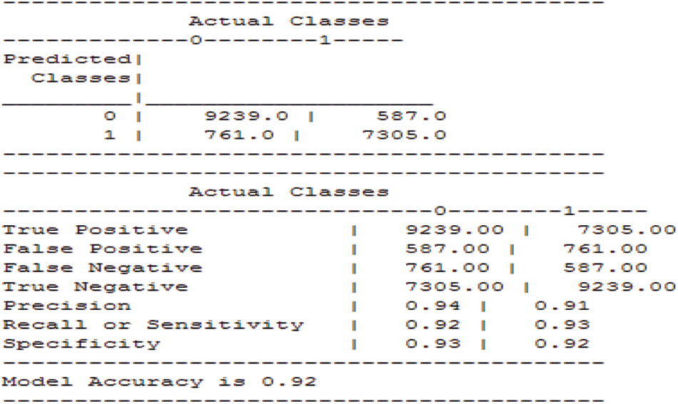
Figure 8: Performance outcome

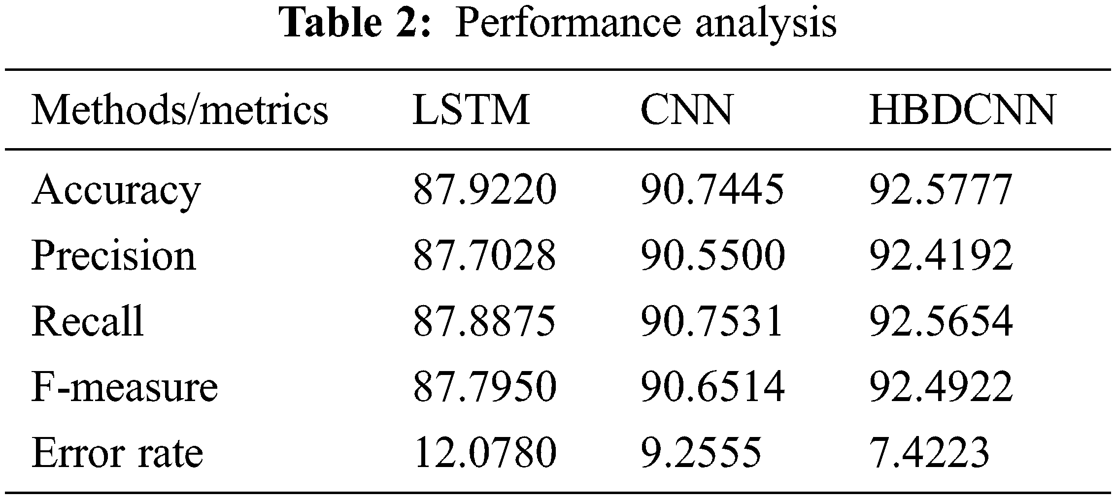
The performance of the existing CNN, LSTM models, and the proposed Half Binomial Distribution Convolutional Neural Network (HBDCNN) are compared in terms of error rate, f-measure, recall, precision, accuracy values are represented in Tab. 2.

4.1 Accuracy

Accuracy is a simple ratio of accurately forecasted observations to total observations. Therefore, it is a nearly straightforward performance metric.

Accuracy=TP+TNTP+FP+FN+TN (16)

The Proposed HBDCNN technique and available CNN and LSTM techniques are compared in terms of accuracy, and its results are shown in Fig. 9. The LDIWCSO algorithm is used in this work for selecting optimum features. For covid-19 prediction, HBDCNN is utilized here, and this prediction is made using selected features. This produces better accuracy. Proposed HBDCNN delivers around 92.57% accuracy value, CNN attains 90.74%, and 87.92% of accuracy is produced by LSTM as indicated in experimental results. Compared with CNN and LSTM techniques, higher accuracy value is produced by the proposed HBDCNN, as shown in test findings.

Figure 9: Accuracy comparison

4.2 Precision

Precision value is defined as the ratio of accurately classified as positive observations to total expected positive observations and it is expressed as,

Precision=TPTP+FP (17)

The Proposed HBDCNN technique and available CNN and LSTM techniques are compared in terms of precision, and its results are shown in Fig. 10. The methods are plotted on the x-axis, and for the y-axis, precision values are plotted. Proposed HBDCNN produces around 92.41% precision value, CNN produces 90.55%, and 87.70% is produced by LSTM as indicated in experimental results. When compared with available techniques, a high precision value is produced by proposed HBDCNN as in test findings.

Figure 10: Precision comparison

4.3 Recall

In covid-19 prediction, recall is a ratio of actual true instances that are retrieved successfully.

Recall=TPTP+FN (18)

The Proposed HBDCNN technique and existing CNN and LSTM techniques are compared in terms of recall, and its results are shown in Fig. 11. It is observed from the graphical evaluation that the proposed HBDCNN attains 92.56% recall value, whereas the existing CNN and LSTM produced 90.75% and 87.88% recall results. Thus, the proposed work outperformed the existing techniques in terms of Recall.

Figure 11: Recall comparison

4.4 F1 Score

Recall and precision’s weighted average produces F1 score. Classifier performance can be rated using this as a statistical measure. False negatives and false positives are taken into account for this score. F1 score is expressed as,

F−measure=2Precision∗RecallPrecision+Recall (19)

The Proposed HBDCNN technique and available CNN and LSTM techniques are compared in terms of F-measure, and its results are shown in Fig. 12. The graphical results showed that the proposed HBDCNN approach attains 92.49% F-measure. Alternatively, the existing CNN and LSTM approach attained 90.65% and 87.79% F-measure respectively. Compared with the existing techniques, a higher f-measure value is produced by the proposed HBDCNN, as shown in experimental results.

Figure 12: F-measure comparison

4.5 Error Rate

Error rate performance of LSTM, CNN and HBDCNN techniques are illustrated in Fig. 13. The error rate of the proposed HBDCNN approach is observed to be 7.4%. Alternatively, the error rate attained by CNN is 9.25% and that of LSTM is observed to be 12.07%. Thus, it is clearly observed that the proposed approach resulted in significant performance with a minimal error rate compared to the existing CNN and LSTM techniques.

Figure 13: Error rate comparison

5  Conclusion

Linear Decreasing Inertia Weight based Cat Swarm Optimization with Half Binomial Distribution based Convolutional Neural Network (LDIWCSO-HBDCNN) is proposed in this work to predict death and confirmed COVID cases. Data is normalized initially using min-max normalization. LDIWCSO algorithm selects the optimum features, which will enhance classification accuracy. The HBDCNN is used for predicting covid-19 according to selected features. Accuracy value around 92.57%, precision value about 92.41%, recall value about 92.56%, f-measure results about 92.49%, and error rate value about 7.4% is obtained using the proposed system as shown in experimental results. The future enhancement of this work would be to use various recent optimization algorithms like Harmony Search (HS) and analyze its performance.

Acknowledgement: We thank anonymous referees for their helpful suggestions.

Funding Statement: The authors received no specific funding for this study.

Conflicts of Interest: The authors declare that they have no conflicts of interest to report regarding the present study.

This work is licensed under a Creative Commons Attribution 4.0 International License, which permits unrestricted use, distribution, and reproduction in any medium, provided the original work is properly cited.