DOI:10.32604/csse.2023.024419
| Computer Systems Science & Engineering DOI:10.32604/csse.2023.024419 | |
| Article |
Wireless Sensor Network-based Detection of Poisonous Gases Using Principal Component Analysis
1Easwari Engineering College, Chennai, 600089, India
2Velammal Engineering College, Chennai, 600066, India
3Velammal Institute of Technology, Chennai, 601204, India
*Corresponding Author: N. Dharini. Email: dharini1990@gmail.com
Received: 16 October 2021; Accepted: 15 December 2021
Abstract: This work utilizes a statistical approach of Principal Component Analysis (PCA) towards the detection of Methane (CH4)-Carbon Monoxide (CO) Poisoning occurring in coal mines, forest fires, drainage systems etc. where the CH4 and CO emissions are very high in closed buildings or confined spaces during oxidation processes. Both methane and carbon monoxide are highly toxic, colorless and odorless gases. Both of the gases have their own toxic levels to be detected. But during their combined presence, the toxicity of the either one goes unidentified may be due to their low levels which may lead to an explosion. By using PCA, the correlation of CO and CH4 data is carried out and by identifying the areas of high correlation (along the principal component axis) the explosion suppression action can be triggered earlier thus avoiding adverse effects of massive explosions. Wireless Sensor Network is deployed and simulations are carried with heterogeneous sensors (Carbon Monoxide and Methane sensors) in NS-2 Mannasim framework. The rise in the value of CO even when CH4 is below the toxic level may become hazardous to the people around. Thus our proposed methodology will detect the combined presence of both the gases (CH4 and CO) and provide an early warning in order to avoid any human losses or toxic effects.
Keywords: Wireless sensor network; principal component analysis; carbon monoxide-methane poisoning; confined spaces
Wireless Sensor Networks (WSN) refers to cluster of sensor nodes co-operatively co-ordinate with each other and helps in reporting sensed data to the network head (sink). Sensed data could be any environmental or structural data such as temperature, humidity, pressure, motion detection, gas, infrared, proximity etc. Behind any WSN network, there are suitable routing, data aggregation, energy harvesting, and security protocols in place for its efficient operation. The role of each and every task stated has its known functionality. WSN structures today play an important role in environmental monitoring. Environmental and toxic gases present in the atmosphere need to be monitored continuously in critical applications like coal mines, drainage systems, chemical plants etc. The amount of data generated from sensors is enormously high. Obviously data generated are from different heterogeneous sensors, this further increases the complexity. Thus any simple technique or algorithm which can aggregate and alert for an event is the current need. One such Data Aggregation technique is Principal Component Analysis (PCA).
PCA is a statistical dimensionality reduction technique, in which the concept behind the principal axis was proposed by Karl Pearson and was later formulated by Harold Hotelling, It is mainly based on eigen values and eigen vectors. The main idea of principal component analysis (PCA) is to reduce the dimensionality of a data set consisting of many variables correlated with each other, either heavily or lightly, while retaining the variation present in the dataset, up to the maximum extent. The same is done by transforming the variables to a new set of variables, which are known as the principal components (or simply, the PCs) and are orthogonal, ordered such that the retention of variation present in the original variables decreases as we move down in the order. It is applicable on linear datasets. It takes in the dataset as its input and computes the covariance among the data and reports the direction of the presence of abundant data. This is a kind of unsupervised learning technique which finds mutually orthogonal directions of greater variance.
Methane-Carbon Monoxide Poisoning
Incomplete combustion in enclosed surfaces may always lead to emission of many toxic gases in the environment such as Carbon Monoxide, Methane, Carbon dioxide, Non-methane hydrocarbons and other green house gases. These toxic gases are capable of polluting the environment and in the worst case may lead to accidental deaths to the humans who come into the exposure of such combustible gases. These gases has a property of inflammability when they exists alone, but once they co exists in an environment above or below certain thresholds they can cause explosions and create various health hazards. During wild forest fires or in underground coal mining or sewage systems, the most toxic gases which people are exposed to are Methane and Carbon monoxide. Individually both the gases have their toxic levels to be checked and reported. But practically their co existence at various situations is hard to study and detect in order to develop a warning system. Particularly methane independently if it exists in a region below or above their threshold value does not pose any harm. But situations in which the oxygen levels gets low it may produce toxic carbon monoxide and create explosions. Thus in cases of forest fires or underground coal mines or sewage systems the oxygen levels being low, there are lots of possibility of Methane-Carbon Monoxide co-existence and poisoning. Upper and Lower Explosive Limits of Carbon Monoxide is specified in Fig. 1.
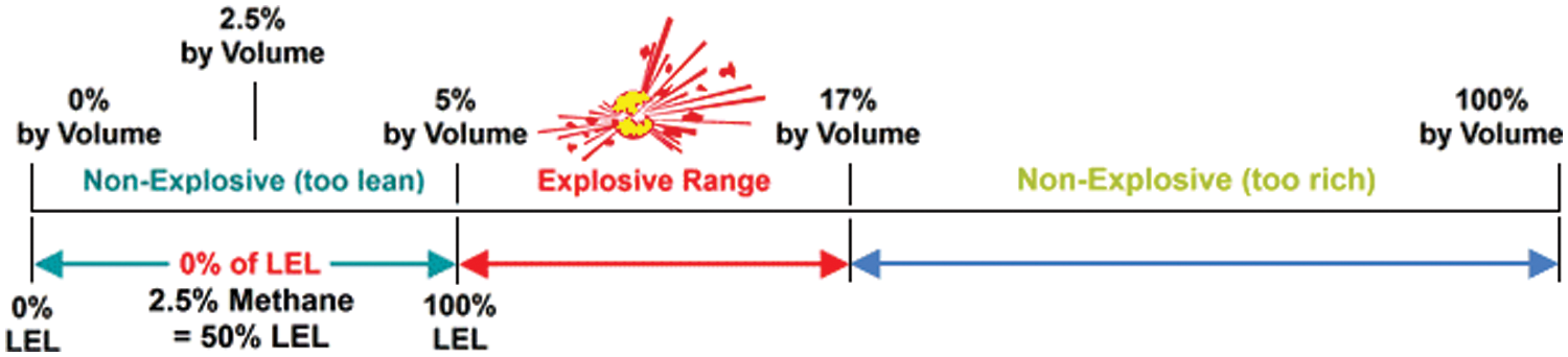
Figure 1: Explosive limits of methane [1]
The properties of Methane and Carbon Monoxide are given below
Methane
• Methane is the simplest organic compound and hydrocarbon with the chemical formula CH4.
• It is colorless, odorless and tasteless gas.
• Methane is not toxic and does not pose any immediate health hazard. But high concentration reduces the presence of oxygen and creates suffocation.
• It becomes flammable when it reaches the concentration of 5%–15%.
• If it burns under insufficient oxygen, toxic carbon monoxide is produced.
Carbon Monoxide
• Carbon Monoxide is a colorless odorless and non irritant gas with chemical formula of CO.
• It is a non corrosive highly poisonous gas.
• It burns in air with bright blue flame.
• It has a molecular weight of 28.01 g/mol.
• Exposure to CO at concentrations over 350 ppm can cause confusion fainting on exertion and collapse.
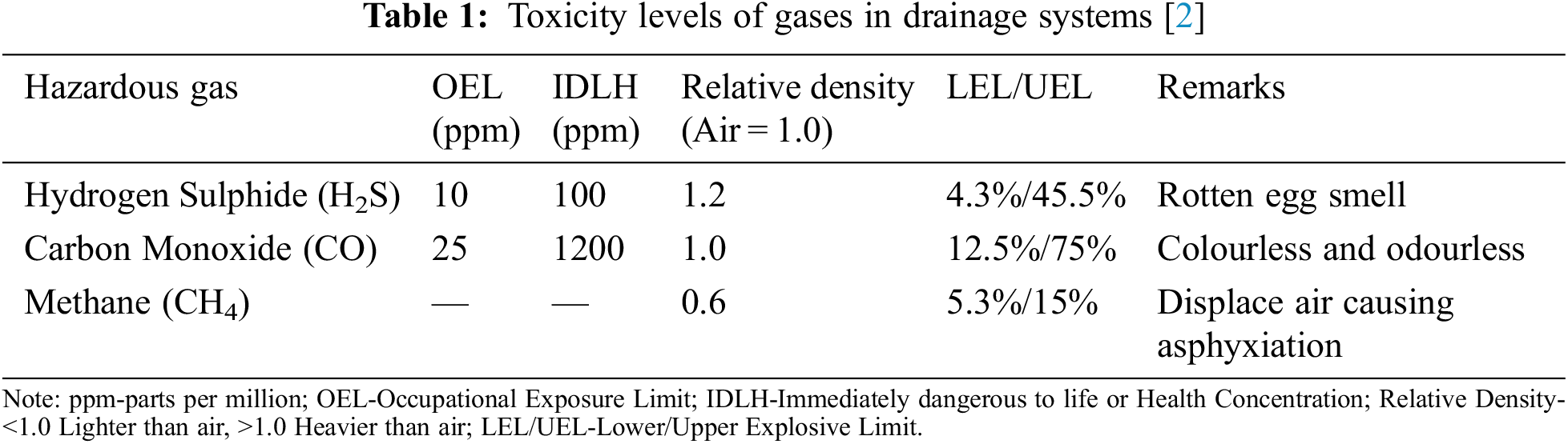
When there is any outburst of fire in an enclosed surface the amount of oxygen levels (O2) gets decreased and at the same instant the outburst of carbon dioxide (CO2) increases thus the combustion process gets altered from one complete combustion to incomplete combustion leading to the emission of carbon monoxide (CO). Based on the report prepared by Occupational Safety and Health Branch, Labour Department in Tab. 1, the toxicity levels of poisonous gases generated in sewage systems is referred.
2 Contribution Towards CH4-CO Poisoning: Problem Statement and Proposed Idea
According to the study conducted by Deng et al. [3], in a paper titled “Experimental and simulation study on the influence of carbon monoxide on explosion characteristic of methane” when CH4 concentration was below the stoichiometric concentration, the addition of CO promote the intensity of gas explosion; oppositely excessive CO would inhibit the gas explosion reaction. The inhibitory effects become more significant as the concentration of CH4 increases. Thus traditionally alerts are triggered when the concentration of gases reaches certain percent of the LEL or UEL limit, such as
1. CH4 reaching the LEL limit of 5% concentration or UEL limit of 15% in air
2. CO reaching the LEL limit of 12% concentration or UEL Limit of 75% in air
But according to the above simulation study by Deng et al. [3] it is indeed necessary to perform correlation study on the sensed values with respect to time to report certain situations such as
Case 1: Both CH4 and CO are steadily increasing with respect to time: high alert of toxicity/explosion
Case 2: CH4 is steadily decreasing (Traditional alert may not be triggered) and CO is increasing but not had reached the LEL limit (Traditional alert may not be triggered), still explosion or toxicity is possible because methane has the property to explode when there is a rise of CO even if it is below the stoichiometric concentration. The influence of CO on CH4 is given in Fig. 2 stated by Deng et al. [3], existing or the state of works were developed to detect the presence of these toxic gases merely by setting a threshold value. Detecting the toxicity towards a particular value may not fit in situations such as forest fires or coal mines or drainage systems because these toxic gases co exists. An increase or decrease of one or the other may lead to unforeseen situations.
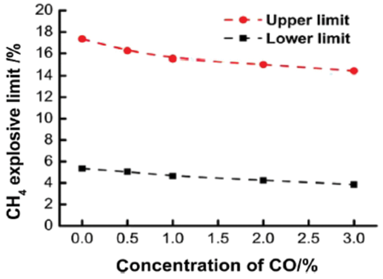
Figure 2: The influence of CO on the CH4 explosive limit [3]
An alert is required in regions at times wherein the value of CH4 may be below threshold value but the amount of CO may be in the increasing scale towards threshold. In such cases both the gases may not have reached their warning levels, so alarms will not be triggered. But chemically speaking if CO is added to methane, even if methane being at low levels it may cause explosion if exposed for a prolong amount of time stated in [3]. If a person is exposed even at low levels of methane and carbon monoxide for a longer amount of time, he may pose to higher risk. Thus a relative study between time, Carbon Monoxide and Methane is very much essential to derive an alert system.
Thus by analyzing the properties of methane and carbon monoxide and their toxic levels, the proposal here is to perform a simulation study on the correlation of both the gases with respect to time instances of their sensing process. The gas levels are sensed every 5 s and the correlation of CO and CH4 is studied for every 20 s. Nodes which are present for prolonged duration along the respective principal component axis zone are identified and alerted in advance. By identifying the regions of correlation, an alert system is derived based on their values.
3.1 Principal Component Analysis
There are many works in the literature related to PCA and its variants in various applications. One such work titled “Data Aggregation with Principal Component Analysis in Big Data Wireless Sensor Networks” by Li et al. [4] finds the optimal number of members in each cluster based on the data magnitude and data correlation. The projection matrix from the principal component analysis is forwarded to the sink instead of forwarding the entire data set. The work is compared with the LEACH and K means Clustering algorithm.
A work by Zhang et al. [5] in a paper titled “An event based Data aggregation scheme using PCA and SVR for WSN”. Data aggregation is performed using PCA. Only the projected data is transmitted during the normal situations. Data aggregator node trains the historical data to obtain a forecasting model and predicts the data using SVR and check the accuracy of prediction. The proposed work reduces the amount of data packets sent from the data aggregator node when event occurs.
Algorithm of Data Compression based on multiple Principal Component Analysis [6] over the WSN by Chen et al. proposed an algorithm that can efficiently remove the correlation between the raw measurements and also between the principal components of the neighbouring cluster heads and improves the data compression ratio thus ensuring the data reconstruction accuracy. PCA is used in clusters at each level iteratively, thus leading to multiple PCA. Comparison is made between single and multiple PCA performance. It ensures good compression ratio and data reconstruction accuracy.
PCA is used as an Intrusion Detection tools in the state of works such as “The Gateway anomaly Detection and Diagnosis in WSN” by Zhen et al. [7] where the communication data of the gateway is analyzed to detect malicious gateway node based on PCA. Based on the error between the current data and reconstructed data and considering T2 statics and Q statistics control limits were set to classify the normal and abnormal data. Real datasets from the cold rolling and continuous annealing line in steel enterprises were used in MATLAB to study the performance. The abnormal state of the system under the running condition was detected and the cause of abnormal variables was diagnosed. Abnormal fault tolerance measure is also presented.
Kernal Principal Component Analysis (KPCA) is used as a natural non linear generalization of PCA. Based on the reconstruction error from the KPCA outliers can be detected. A work by Ghorbel et al. [8] in “A novel outlier detection based on one class principal component classifier in WSN” used Mahalanobis distance to calculate the mapping of data points in the feature space to separate outlier points from the normal pattern. On the projected dataset from PCA if the Mahalanobis distance of a node is greater than or equal to Maximum thresholds of Mahalanobis distances it is classified as normal else it is an outlier.
Recursive PCA [9] based multivariate fault tolerant Data Aggregation in WSN was proposed by Tianqi et al. in which PCA is applied recursively at various time instances in which covariance matrix, eigen values and vectors are updated recursively. CH collects the multivariate data and reorganizes the data based on the physical properties and apply R-PCA over the newly projected data matrices to avoid faults. Fault detection accuracy is improved by 20% and reconstruction error is reduced by 28%.
Thus PCA has been extensively used in literature as an Intrusion Detection System and Data Aggregation tool. Our work aims to use PCA as a tool to detect the poisoning effects of CH4-CO by obtaining the direction of the principal component data, eigen vectors and the presence of the data along the different axis.
A work by Fahim et al. [10] presents a CO poisoning prevention based on WSN which detects the CO level in a restrained space like steel mills and upon alarming conditions counter measure is activated. If the CO concentration crosses the threshold value of 300 ppm the actuator circuit comes into play the system has online data logging in MySql Database. The actuator circuit controls the exhaust system via a relay circuit and upon the reception of the activation signal the respective exhaust ON. Effect of the actuation circuit is studied.
Development of Wireless Sensor Network for Environmental Gas Monitoring [11] by Somava et al. for early gas leak detection and fast operator alarm. The system is designed to accurately measure the methane concentration in the atmosphere by using semi conductor sensors realized on membranes. Type C or Type D batteries can be used to increase the lifetime upto 5 times of the baseline. It is also found that the maximum sensor sensitivity to methane is achieved by heating sensor up to 525 degree celcius. This work demonstrated the optimization of gas measurement, Data processing and Data transmission thus reducing the power consumption of nodes.
The ill effects of CO and CH4 are studied in the literature [12] in an online article “Relevance To Public Health” where the environmental exposure of CO in United states. Ill effects on human animals and the developmental effects were summarized. High levels of CO produce toxicity of central nervous system and causes headache, nausea, dizziness, vomiting, disorientation etc. The human equivalent exposure concentrations are approximately 32 ppm (COHb = 5%) and 160 ppm (COHb = 20%). The study summarizes the effect of Blood Carbohemoglobin levels corresponding to Adverse Health effects of CO.
A work by Peng et al. [13] titled ‘A wireless sensor data-based coal mine gas monitoring algorithm with least squares support vector machines optimized by swarm intelligence techniques’ proposed a least square support vector machine algorithm to process and classify the wireless sensed data values. Several particle swarm optimization techniques were used to tune the hyper parameters of the least square support vector machines. Extensive simulations were carried out using several smaller and bigger datasets obtained from UCI machine learning repositories. Swarm Intelligence based classification technique provided higher accuracy of classification for high dimensional datasets with more categories, but required room for improvement with small dimensional datasets.
A work which inspired my proposal was “Experimental and Simulation studies on the influence of carbon monoxide on explosion characteristics of Methane” by Peng et al. [13] state that the explosion characteristics parameters of CH4 and the mixture are similar. When CH4 concentration was below the stoichiometric concentration, the addition of CO could promote the intensity of gas explosion, oppositely CO could inhibit gas explosion reaction. With increase of CO the upper and lower explosive limits decrease.
Design and evaluation of a wireless sensor network for Mine Safety Monitoring was proposed by Niu et al. [14] developed a heterogeneous hierarchical prototype for monitoring safety of mines. Overhearing based adaptive data collection scheme was introduced. Correlation in both time and space was taken into account. Concentration of Methane in mines is collected using the overhearing principle. In order to address the network traffic issue and also to reduce the offset error which occurs while reporting sensed data thus causing delay, the overhearing based adaptive data collection scheme was developed. The authors claim to achieve maximum coverage in corridor environment with dozen of sensors and can also be applicable to coal mine safety monitoring aiming to provide fault tolerance, reliability and maintainability.
3.3 Drawbacks of the Existing Works
Current Monitoring approaches necessitate real-time sensing and decision making through WSN. Existing or the state of work works were developed to detect the presence of these toxic gases merely by setting a threshold value. The prevailing approaches often make use of SQL (Structured Query Language) like primitives by using a sub event list and confidence functions in SQL. SQL based monitoring cannot capture data dependencies and interactions among different sensing scenarios. It cannot support probability models and collaborative decision making. Detecting the toxicity towards a particular value may not fit in situations such as forest fires or coal mines or drainage systems where the toxic gases co exists. An increase or decrease of one or the other may lead to unforeseen situations. A quantitative and collaborative decision making system is required to report emergencies.
While applying these concepts in real time, there will be many situations in which threats may be imparted into the network to capture such toxicity reporting networks to create wrong alerts. Thus by analyzing the properties of methane and carbon monoxide and their toxic levels, the proposal here is to perform a simulation study on the correlation of both the gases with respect to time instances of their sensing process. The gas levels are sensed every 5 s and the correlation of CO and CH4 is studied for every 20 s. Nodes which are present for prolonged duration along the respective principal component axis zone are identified and alerted in advance. By identifying the regions of correlation, an alert system is derived based on their values.
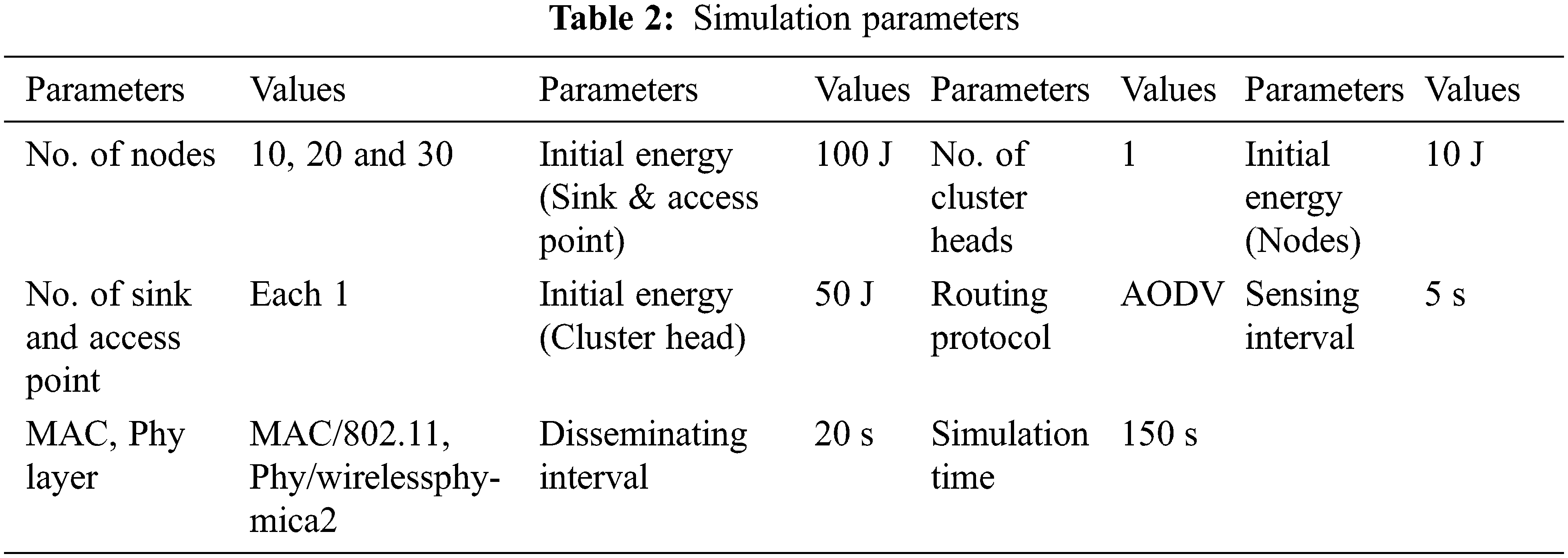
Static and Heterogeneous cluster based sensor network with Methane and Carbon Monoxide sensors are deployed randomly in the area of 30 m ∗ 30 m. Routing protocol used is AODV.
• Initial energy of sensor node—10 J
• Initial energy of cluster head node—50 J
• Initial energy of sink node—100 J
PCA is a statistical dimensionality reduction technique, in which the concept behind the principal axis was proposed by Karl Pearson and was later formulated by Harold Hotelling, It is mainly based on eigen values and eigen vectors. The main idea of Principal Component Analysis (PCA) is to reduce the dimensionality of a data set consisting of many variables correlated with each other, either heavily or lightly, while retaining the variation present in the dataset, up to the maximum extent. The same is done by transforming the variables to a new set of variables, which are known as the principal components (or simply, the PCs) and are orthogonal, ordered such that the retention of variation present in the original variables decreases as we move down in the order. It is applicable on linear datasets. It takes in the dataset as its input and computes the covariance among the data and reports the direction of the presence of abundant data. This is a kind of unsupervised learning technique which finds mutually orthogonal directions of greater variance.
Step 1: Normalize the data
First step is to normalize the data. This is done by subtracting the respective means from the numbers in the respective column. So if we have two dimensions X1 and X2, all X1 become X1∼ and all X2 become X2∼. This produces a dataset whose mean is zero.
Step 2: Calculate the covariance matrix: Since the dataset we took is 2-dimensional, this will result in a 2 × 2 Covariance matrix which is calculated using Eqs. (1) and (2).
If the data sets considered are of different scales and expressed in different units, correlation matrix need to be formulated, for which the eigen values and eigen values need to be found. In this case since both the data are expressed in percentage of concentration present in the air, co variance matrix will suffice this situation
Step 3: Calculate the eigenvalues and eigenvectors of the co-variance matrix. Eigen values and vectors are calculated using determinant matrix by using Eq. (3)
where I is the identity matrix of the same dimension as A (Covariance Matrix). For each eigenvalue ƛ, a corresponding eigen-vector “v” can be found by solving Eq. (4)
Step 4: Choosing components
We order the eigen values from largest to smallest so that it gives the components in order or significance. If we have a dataset with “n” variables, then we have the corresponding “n” eigenvalues and eigenvectors. For eigen values ƛ1 and ƛ2, let the eigen vectors be [x1, x2]T and [y1, y2]T. The eigen vector [x1, x2]T corresponds to the principal component axis 1 which contains maximum amount of information. The eigen vector [y1, y2]T contributes to minimum amount of information, corresponding to PC2 which is mostly ignored due to less amount of information.
The percentage of information present in each component is calculated and the PC (Principal Component) containing least amount of information is ignored. Total Sample Variance is calculated using Eqs. (5) and (6).
The contribution made by the found eigen values is calculated using Eqs. (7) and (8).
Thus % of variance contributed by first eigen value
% of variance contributed by second eigen value
Step 5: New dataset with principal components.
The reduced dataset obtained after performing PCA is constructed using Eqs. (9) and (10).
where
4.1.3 Methane-Carbon Monoxide Poisoning Detection Model
In order to confirm the data correlation between two different sensed values, Pearson correlation coefficient is calculated between the two types of data as in Eq. (11) Pearson Coefficient Value lies between 0 and 1.
If the coefficient is positive, CH4 and CO has a positive relationship between them, i.e., if one increases, the other also gets increased. If the coefficient is negative, CH4 and CO have negative relationship between them, i.e., if one increase, the other may decrease.
In order to identify the nodes lying along the different axis and most importantly to identify the region of the abundant data, PCA is performed. The output of any PCA process will provide various principal component axis in the decreasing order, where each axis represent the region of abundant data containing the principal components namely PC1 (Principal Component 1), PC2 (Principal Component 2) etc. PC1 usually contains the most important data. PC2 has the least important data. Having 2 data sets (CH4 and CO), a maximum of only 2 PCs are possible.
Every 5 s, both CH4 and CO data are sensed and every 20 s nodes disseminate their data to the Cluster Head. Each Cluster Head performs PCA over the data every 20 s.
Heterogeneous network with two different types of sensors (CH4 and CO) are deployed. Having studied the characteristics of Methane and Carbon Monoxide, based on the following graph the alert regions are identified and by formulating and obtaining the principal component axis of the data; along which maximum data present is identified.
Oxygen levels also play a vital role in creating toxicity and explosion in regions where carbon monoxide and methane co exists, if there is sufficient oxygen or if the region is oxygen rich, the explosion can be avoided. Having considering the work towards poisoning detection in regions such as sewage systems, forest fires and underground coal mines, these regions cannot be highly oxygen rich because sewage and underground mines are enclosed surfaces where they may be only optimal oxygen level and during forest fires, oxygen levels may go down. So let us assume that the regions under study has required amount of oxygen (i.e., 19.5%) but they are not oxygen rich. According to the source [12] reference level is set as 19.5%.
4.1.4 Categorization of Toxic and Explosive Regions
The Fig. 3a illustrates how we categorize each region based on the data present along the region. The regions are categorized in such a way that how CH4 values tend to change with respect to increase or decrease of CO.
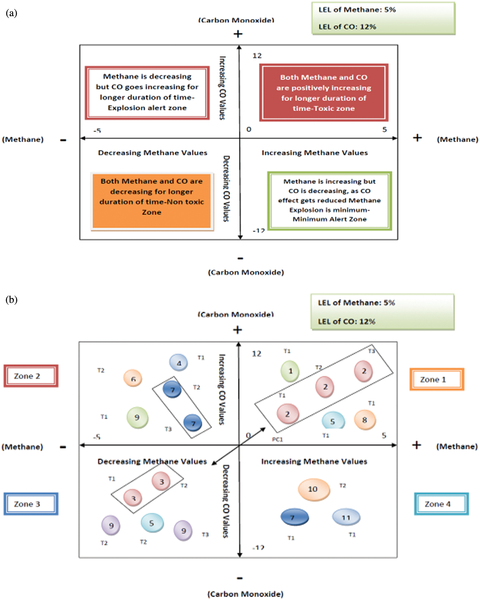
Figure 3: (a) Graph showing categorization of zone based on plotted values (b) Example graph showing nodes present in proposed categorized zones
In Zone 1 both CO and CH4 are increasing, the increase of one or the other even below the Lower Explosion Limit shows an increasing trend in the data over a period of time. The nodes which are present for a long time in this region may have an increasing trend of data. Thus there is a possibility of toxicity being created in this region. Nodes which are present in this region for a longer amount of time are identified as toxic region nodes and alert is triggered.
In Zone 2 CO has an increasing trend of values, but methane concentration is below the stoichiometric concentration, since both CO and CH4 are below their LEL limit traditional alert systems may not trigger an alert, but as per the experimental study conducted [3], even if CH4 is below their LEL, addition of CO may increase their explosiveness. Thus the nodes which are lying for longer duration of time are identified as explosive region nodes and alert is triggered.
In Zone 3 both CH4 and CO have a decreasing trend of data over a period of time this reduces their toxicity and explosive characteristics, thus it is a non toxic region.
In Zone 4 methane data alone is increasing, since CO addition is decreasing the possibility of explosive behavior of methane is reduced. Toxicity may increase due to the addition of methane along this region, so nodes lying in this area need to be constantly monitored for their methane values in order to avoid toxicity. Thus this is a minimum alert region.
The zone where PC1 is present is alerted according to the above categorization.
The steps are as follows
1. Perform PCA
2. Identify the region of maximum data (abundant data) i.e., PC1
3. Plot the mean adjusted data values with data points with corresponding Node identifier in GNUPLOT
4. Plot the PC values: PC1 and PC2 in GNUPLOT
5. PC1 and PC2 will lie along any of the four regions: Zone 1 or 2 or 3 or 4
6. Based on the region along which PC1 and PC2 are present; alerts are triggered for the corresponding regions.
Data values are plotted along with their node id and sensed time instance values. As in Fig. 3b below, we could see node 2 is present in the zone 1 for various time instances (node 2 repeats) and it also lies along the principal component axis, thus node 2 is under the toxic zone. Next in zone 3, node 3 is present for longer duration of time at various time instances (node 3 repeats) and also along the principal component axis, thus node is in the non-toxic zone. We could see node 7 (zone 2) in the explosive zone for longer duration of time.
4.1.5 Pseudocode: Determining the Node Presence Along Different Regions
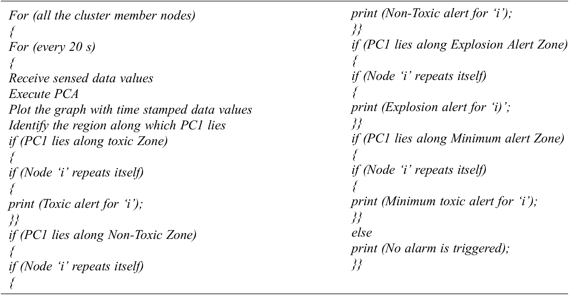
Simulations were carried out using NS2-Mannasim framework [15] with Mica2 mote characteristics AWK scripts were used to analyze the tracefiles generated. Simulation parameters were set as in Tab. 2.
5.1 Principal Component Analysis with 10, 20, 30 Number of Nodes, 50% CH4 Nodes and 50% CO Nodes
The NAM (Network Animation) Window showing the node deployment considered for execution of PCA process is shown in Fig. 4a. Methane and Carbon Monoxide sensor pairs were assumed to be located at the same location. So that the correlation formulated makes sense in real time while they report data values. Terminal Output in Fig. 4b depicts the percentage of the principal data lying along each axis from the derived eigen values and eigen vectors. Eigen value 1 contributes 85% of the total principal data, which implies that most of the sensed values range in the zone of Toxic and Non Toxic Region. Eigen value 2 contributes to 15% of the Principal data which means rest of the sensed data contribute to the Explosive and Minimum alert zone. Nodes present in corresponding regions can be identified by means of GNU Plot [16].
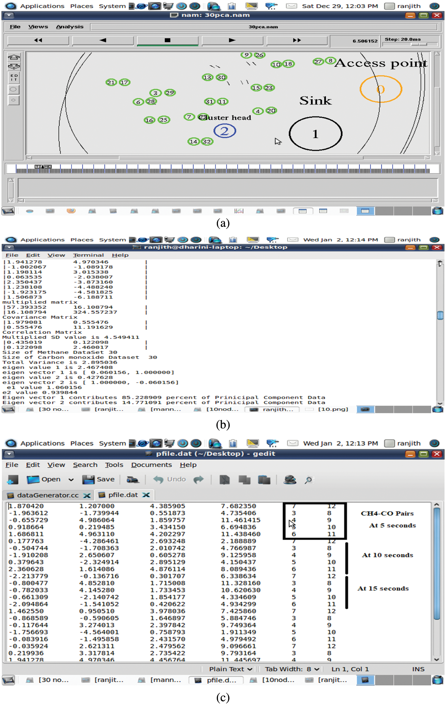
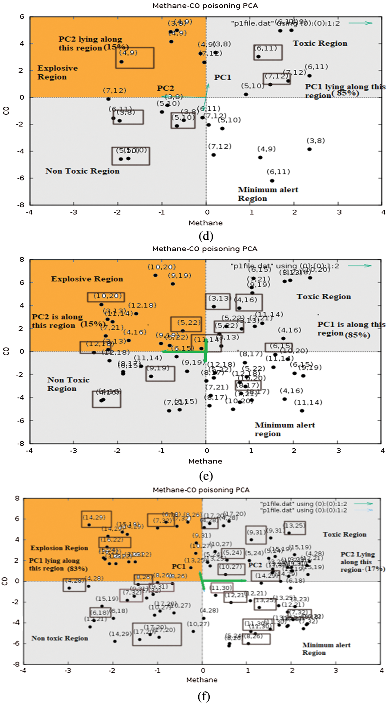
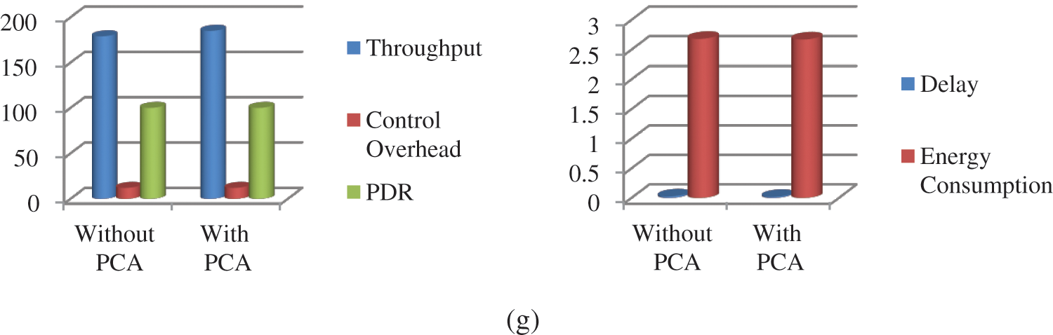
Figure 4: (a) NAM window showing the node deployment and communication happening among them (b) PCA terminal output showing eigen vectors and eigen values found and the % of contribution of principal component data (10 nodes) (c) Date file generated during PCA with reduced and original data matrix and CH4-CO node ID pairs (10 nodes) (d) GNU plot (10 nodes) showing the nodes present in different regions with PCA axis shown (e) GNU plot (20 nodes) showing the nodes present in different regions with PCA axis shown (f) GNU plot (30 nodes) showing the nodes present in different regions with PCA axis shown (g) Performance analysis
Data file is generated to create the GNU Plot [16] from which sensed values and the PCs’ (Principal Components) can be visualized as shown in Fig. 4c. The first two columns in Fig. 4c represents the reduced datasets of CH4 and CO respectively. The 3rd and 4th column represents the original sensed values of CH4-CO pairs. 5th and 6th columns represent the CH4-CO Node pair IDs’. Sensing is done every 5 s; PCA is carried out every 20 s. Thus Node Pairs IDs’ gets repeated every 5 s. Node Pair IDs’ which repeats itself along each region represents that those pairs lie along the region for prolonged time instances.
Methane and Carbon Monoxide sensor pairs were assumed to be located at the same location. So that the correlation formulated makes sense in real time while they report data values. Fig. 4d includes the GNU Plot with representation of each PC's contribution in terms of the percentage of the principal data lying along each axis from the derived eigen values and eigen vectors.
From the plot in Fig. 4d we have plotted the reduced data values with their corresponding node id pairs. As per our formulation the regions have been divided. Based on the direction where maximum data is present, alert can be triggered. Node ID pair that repeat themselves in each region is marked with rectangle and those rectangle nodes are to be alerted. For example in Fig. 4d PC1 (Principal Component 1) is lying along the Toxic and Non Toxic Region contributing to 85% of data. Node ID pairs (6, 11) and (7, 12) lie along the Toxic Region. Node ID pairs (5, 10) and (3, 8) lie along the Non Toxic Region. Thus Nodes (6, 11) and (7, 12) needed to be reported for their increasing trend in Toxicity. Similarly PC2 (Principal Component 2) lie along Explosive and Minimum Alert Region contributing to 15% of Data. Thus Node ID pairs (4, 9) repeats itself and need to be reported for its Explosiveness. The similar GNU Plots for 20 and 30 Number of nodes are shown in Figs. 4e and 4f.
Datasets includes random data generated by the sensor nodes following normal, uniform and exponential distribution. Plotting the data in GNU Plot becomes easier to visualize the nodes present in each zone. Identifying the nodes present in areas of toxicity, explosion and minimum alert region with a simple statistical technique without any loss of wireless sensor network performance metrics proves the efficiency of the proposed PCA based Poisoning detection algorithm. When the scalability of the network increases, GNU Plot may cause overcrowding effect, still better plotting graphs are available in the market, those softwares can be replaced in the place of GNU Plots. On the other hand clusters can be increased and each cluster PCA Plot can be generated individually to account for scalability and to reduce the crowding effect.
AWK Scripts were generated and run over the trace files of an ideal heterogeneous and PCA enabled WSN. Performance is compared over Throughput, PDR, Control Overhead, Delay and Energy consumption and shown in Fig. 4g.
Ideal and PCA enabled Network report similar network characteristics thus PCA does not incur any unnecessary overhead or degrade the performance of the network much.
Principal Component Analysis is carried out over the CH4 and CO sensed values. Based on the formulation of the regions and identified Principal Component axis; nodes present in Toxic, Non Toxic, Explosive and Minimum Alert Region were identified by GNU Plot and reported for either Toxicity or Explosiveness. Simulation study of the proposed work with PCA does not confirm the real time detection of CH4-CO poisoning. Sensors need to be deployed in real time to verify the conformity of PCA over such data. But this framework will definitely remain as a prototype for developing such real time emulations and the novelty of segregating the regions based on the toxic and explosive levels will remain unique from other state of works.
Funding Statement: The authors received no specific funding for this study.
Conflicts of Interest: The authors declare that they have no conflicts of interest to report regarding the present study.
1. M. G. Zabetekis, “Methane Explosion Limits,” Gas Data Book, 7th edition, Matheson Gas Products, and from Bulletin 627, Flammability Characteristics of Combustible Gases and Vapors, U.S. Department of the Interior, Bureau of Mines, pp. 2–4, 2001. [Online]. Available: https://www.osti.gov/servlets/purl/7328370/. [Google Scholar]
2. Prevention of gas poisoning in drainage work by Occupational Safety and Health Branch, Occupational Safety and Health Council Labour Department, 2007. [Online]. Available: https://www.labour.gov.hk/eng/public/oh/Drainage.pdf. [Google Scholar]
3. J. Deng, F. Cheng, Y. Song, Z. Luo and Y. Zhang, “Experimental and simulation study on the influence of carbon monoxide on explosion characteristic of methane,” Journal of Loss Prevention in the Process Industries, Elsevier, vol. 36, pp. 45–53, 2015. [Google Scholar]
4. J. Li, S. Guo, Y. Yang and J. He, “Data aggregation with principal component analysis in big data wireless sensor networks,” in Proc. of 12th Int. Conf. on Mobile Adhoc and Sensor Networks, Hefei, China, pp. 45–51, 2016. [Google Scholar]
5. X. Zhang, H. Wu, Q. Li and B. Pan, “An event based data aggregation scheme using PCA and SVR for WSN,” in Proc. of IEEE 85th Vehicular Technology Conf., Sydney, NSW, Australia, pp. 1–5, 2017. [Google Scholar]
6. F. Chen, F. Wen and H. Jia, “Algorithm of data compression based on multiple principal component analysis over the WSN,” in Proc. of IEEE 6th Int. Conf. on Wireless Communication Networking and Mobile Computing, Chengdu, China, 2010. [Google Scholar]
7. F. Zhen, F. JingQi and S. Wei, “The gateway anomaly detection and diagnosis in WSN,” in Proc. of Chinese Control and Decision Conf., Yinchuan, China, pp. 2401–2406, 2016. [Google Scholar]
8. O. Ghorbel, M. Abid and H. Snoussi, “A novel outlier detection based on one class principal component classifier in WSN,” in Proc. of 29th Int. Conf. on Advanced Information Networking and Applications, Gwangju, Korea(Southpp. 70–76, 2015. [Google Scholar]
9. T. Yu, X. Wang and A. Shami, “A novel R-PCA based multivariate fault tolerant data aggregation in WSNs,” in Proc. of IEEE Int. Conf. on Communications, Kuala Lumpur, Malaysia, pp. 1–5, 2016. [Google Scholar]
10. M. Fahim Jan, Q. Habib, M. Irfan, M. Murad, K. M. Yahya et al., “Carbon monoxide detection and autonomous countermeasure system for a steel mill using wireless sensor and actuator network,” in Proc. of 6th Int. Conf. on Emerging Technologies, Islamabad, Pakistan, pp. 405–409, 2010. [Google Scholar]
11. A. Somova, A. Baranovb, A. Savkinb, D. Spirjakinb, A. Spirjakinb et al., “Development of wireless sensor network for combustible gas monitoring,” Sensors and Actuators A: Physical, Elsevier, vol. 171, pp. 398–405, 2011. [Google Scholar]
12. Relevance To Public Health, Guide to atmospheric testing in confined spaces, RAE systems, Honeywell, 2006. https://afcintl.com/wpcontent/uploads/docs/RAE%20pdfs/rae/ap206.pdf. [Google Scholar]
13. C. Peng, Y. Xie, J. Pei and Z. Dezheng, “A wireless sensor data-based coal mine gas monitoring algorithm with least squares support vector machines optimized by swarm intelligence techniques,” International Journal of Distributed Sensor Networks, vol. 14, pp. 1–20, 2018. [Google Scholar]
14. X. Niu, X. Huang Z. Zhao, Y. Zhang, C. Huang et al., “The design and evaluation of a wireless sensor network for mine safety monitoring,” in Proc. of the IEEE Global Telecommunications Conf., Washington, DC, USA, pp. 1291–1295, 2007. [Google Scholar]
15. NS2 Mannasim Framework Home Page. [Online]. Available: http://www.mannasim.dcc.ufmg.br/. [Google Scholar]
16. T. Williams and C. Kelley, ”Labels, Lines, Linespoints, Points, Plots, Print,” in Gnuplot 4.4: An interactive Plotting Program, pp 51–87, 1986. [Online]. Available: http://www.gnuplot.info/docs_4.4/gnuplot.pdf. [Google Scholar]
 | This work is licensed under a Creative Commons Attribution 4.0 International License, which permits unrestricted use, distribution, and reproduction in any medium, provided the original work is properly cited. |