An Ophthalmic Evaluation of Central Serous Chorioretinopathy

L. Shoba; P. Kumar

doi:10.32604/csse.2023.024449

1Department of Information Technology, Jeppiaar Engineering College, Chennai, 600119, India
2Department of Computer Science and Engineering, Sri Krishna College of Engineering and Technology, Coimbatore, 641008, India
*Corresponding Author: L. K. Shoba. Email: lkshoba04@gmail.com
Received: 18 October 2021; Accepted: 05 January 2022

Abstract: Nowadays in the medical field, imaging techniques such as Optical Coherence Tomography (OCT) are mainly used to identify retinal diseases. In this paper, the Central Serous Chorio Retinopathy (CSCR) image is analyzed for various stages and then compares the difference between CSCR before as well as after treatment using different application methods. The first approach, which was focused on image quality, improves medical image accuracy. An enhancement algorithm was implemented to improve the OCT image contrast and denoise purpose called Boosted Anisotropic Diffusion with an Unsharp Masking Filter (BADWUMF). The classifier used here is to figure out whether the OCT image is a CSCR case or not. 150 images are checked for this research work (75 abnormal from Optical Coherence Tomography Image Retinal Database, in-house clinical database, and 75 normal images). This article explicitly decides that the approaches suggested aid the ophthalmologist with the precise retinal analysis and hence the risk factors to be minimized. The total precision is 90 percent obtained from the Two Class Support Vector Machine (TCSVM) classifier and 93.3 percent is obtained from Shallow Neural Network with the Powell-Beale (SNNWPB) classifier using the MATLAB 2019a program.

Keywords: OCT; CSCR; macula; segmentation; boosted anisotropic diffusion with unsharp masking filter; two class support vector machine classifier and shallow neural network with powell-beale classifier

At present, there are two hundred million blind or impaired people around the world, and their quality of life can greatly deteriorate. Roughly 80 percent of current vision deficiency is due to a variety of visual problems which can be prevented, slowed, or cured by the implementation of current information and technology [1]. In the case of the OCT image, an essential diagnostic method for ophthalmology is analyzed and interpreted, and extensive research in this phase is ongoing. The first important thing to determine the course and effect of an illness concerning any procedure is to know the natural history of the disease and to determine whether a therapeutic mode is currently different from the natural history. In CSCR, we have carried out a Pub Med search to find information about the natural history of visual results. This technological progress improves the diagnosis of disease and clinical care efficiency.

Many scientists have suggested various techniques to detect CSCR. Image processing techniques are extensive to retrieve more specific information or produce an optimized image from the raw image of the input. Image recognition techniques also play an important part in CSCR detection. However, target identification and investigation of 3D imagery is the key role of image processing [2]. The CSCR imaging method helps the eye doctor to detect and diagnose various abnormal variations of the macula. Imaging enhancement methods are also used in general medical cases, cancer, and other clinical initiatives [3].

The function of threshold separations from the neighboring image points has reduced the contrast to the image by composing form typically of the brightest point and darkest areas [4]. The filtering technology is used to boost bright spots and dark areas to solve this problem. Pre-processing step is critical because the performance of the process is dependent on image quality, such as segmentation and extraction. To minimize the noise in the images, some filtering techniques are used. Noise reduction procedures are also used for the prevention of noise from various database medical images. It also concentrates on changing those properties of an image that is useful to evaluate the noise types in the particular image [5].

In [6–8] Markov Boundary model was implemented for calculating retinal thickness. Here the image is filtered with a median filter to eliminate speckling noise and filtering from column to column. This technique has the merit of scientifically being used for its precise estimation of thickness. The median filter also eliminates those image properties and causes blurring. A new filtering algorithm has been implemented to minimize the noise in the imaging method [9]. The noise was removed in this paper with the help of Gaussian Retinal Pigment Epithelium (RPE) and Retinal Nerve Fiber Layer (RNFL) filter. It is intended to eliminate the high-pixel RNFL complex since the pixel of the background is identical to the image and then RPE layer segmentation is facilitated. The bilateral filtering image reduction technique has been used to increase the thickness of the RNFL in the OCT images input. In the proposed system, the Gamma noise model is often used to suppress noises in the input OCT image.

The survey investigates various new methods for optimizing and enhancing image properties, such as precision and sensitivity, Accuracy using various value comparative criteria. The various algorithms proposed recently for image attribute enhancement, classification, and detection are discussed. Segmentation can be done in several ways: Pixel, region, edge, model-based, etc [10].

A comparative analysis of different image extraction algorithms in image processing methods was developed [11,12]. They observed 18 CSCR patients and found that the OCT imaging technique is more efficient because it offers accurate data about morphological and retinal changes. CSCR is a condition that mostly affects the macula layer and affects people aged between 20 to 50. In [13] a method for identifying and extracting retinal layers for the analysis, by an adaptive booster, for Cystoid Macular Edema (CME) has been implemented. It also includes evaluating the thickness of individual layers to better diagnose them and to misclassify them, resulting in noise at the output.

In [14] the main problem concerning the quality of the gradation technique was described. The filter and Fuzzy C extraction approach are used to detect exudates. A further Support Vector Machine (SVM) process is used to classify retinal fundus images into Non-proliferative Diabetic Retinopathy (NPDR) and Proliferative Diabetic Retinopathy (PDR). In [15] a fully automated Neutrosophic transformation and graph based shortest path method to segment cyst regions from Diabetic Macular Edema (DME) affected OCT scans has been proposed. A proposed functional shape framework for quantitative shape variability analysis in OCT images has been described. The proposed approach uses surface geometry methods and retinal layer thickness for identifying the anatomical shapes with the help of registration method.

In [16,17] a proposed multi scale convolutional neural network ensemble for the Macular OCT classification has been described. A Computer Aided Diagnosis based on a Multi-scale Convolutional Mixture of Expert (MCME) ensemble model to identify normal retina and two types of macular pathologies. The overall survey clearly explained the demerits for prediction of the abnormalities in OCT image. To overcome these flaws we developed a novel technique. The suggested method’s main goal is to improve accuracy and reduce false-positive predictions. The recent contribution of our proposed work can be outlined as follows:

• For Image Enhancement a proposed Algorithm called BADWUMF is used which should be compared with three different existing algorithms.

• Important features such as point, line and Region and Gray-Level Co-Occurrence Matrix (GLCM) are extracted.

• For Image classification two algorithms namely TCSVM Classifier and SNNWPB Classifier are used.

• The proposed model accurately classifies the Normal/CSCR image on OCT. Image Retinal Database and in-house clinical database will provide a remarkable output.

The paper is outlined as follows: Section 1 focuses on the proposed framework’s introductory section as well as the findings of several academic articles, Section 2 emphasizes the proposed framework, and Section 3 presents the simulation findings and discusses them and Section 4 ends the document.

Fig. 1 shows the proposed system for the OCT image methodology. This system can be divided into three processing phases: Image preprocessing, feature extraction, and image classification. First, the image is preprocessed and the second step is to extract the features. Finally, the classification step is followed by the output. The image is classified by the classification method as a normal or CSCR case. The publicly available CSCR and normal retinal images [18] are used for the analysis of the proposed method as well as clinical database images taken from Madurai hospital, department of ophthalmology, India. The images of the two datasets above are compiled in JPEG formats for this research work which contains 150 images of various eyes with a low noise-to-signal relationship. It includes both Normal retinal images as well as a CSCR image. Initially, Retinal OCT images are used as input to the preprocessing module to delete the unwanted portion of the image [19]. Apply to normal images as well as CSCR retinal database images, the pre-processing phase built to provide four filter types, namely Adaptive median filter (AMF), Adaptive histogram equalization (AHE), Mean filter (MF), and finally BADWUMF. The peak signal to noise ratio, signal to noise ratio, mean square, and structural similarity index ratio are then used to perform a comparison.

The second stage involves extracting functions in an image that will be used for further classification to classify the structure, color, lines of interest, thickening, etc. The most important thing for detecting boundaries is to remove the characteristics of the image such as corner extraction, surface extraction, etc. Here we can extract important features such as point, line, and region. With various algorithms, both of these features can be extracted. The points can be sensed with detect Surf. The Maximally Stable Extremal Regions (MSER) identifies regions and detects the number of lines by the corner function. The final step is to classify the image, using a Two-class Support Vector Machine classifier and a Shallow Neural Network with Powell Beale Classifier that provides better precision in classifying the retinal OCT images as CSCR cases and normal cases. Finally, output values such as accuracy, precision, error, sensitivity, and specificity are also measured.

Medical image databases are critical for stimulating Research & Developing activities in the medical sector. In this research article total of 150 retinal OCT images are tested in both public databases and in-house clinical datasets. OCT Image Retinal Database consists of a total of 450 images. Then the clinical database consists of 250 OCT images obtained from the Department of Ophthalmology, Madurai Medical College, India. For classification, testing the sample of around 150 images is used.

It is a method for modifying the image composition, degree of contrast, and intensity value to increase image quality. The aim is to remove unwanted sounds, thus enhancing image quality. CSCR recognition in retinal images relies on steps taken in the pre-processing initial period. Input image noise is eliminated by the respective preprocessing steps. Preprocessing is a generic name for lowest-level image strength input and output processes [20]. To remove the noise, image enhancement is used which includes AMF, AHE, MF and finally BADWUMF.

The image is bought from a camera or other imaging device, it is always difficult to use the perspective from which it is intended. More precise information on the image of the camera may be distorted before final processing by the noise, random changes in intensity, lighting, or limited contrast. Various types of filters, including linear or non-linear filters, variants, or non-linear filters, are available. The principal downside for local averages is to have sharp discontinuities in image intensity. A median of the grey values of the local population is the optimal option. These filters are called median filters and are very qualified to eliminate noise, pulse, and salt, while preserving image detail. The filters are also referred to as median filters. The Regular Median Filter does not perform well where the pulse noise is less than 0.2, although the adaptive median filter can tolerate certain noises better [21]. The adaptive median filter retains a detailed and smooth non-impulsive noise, whereas the normal median filter is not maintained. The input OCT image with an adaptive median filter is excluded from the impulsion noise here. It is executed as follows.

• The noise pixel g(x, y) are detected by comparing the simple thresholds and averages around the target pixels.

• Select the 3 × 3 window centered at the noise pixels g(x, y). If there exist informative pixels around g(x, y), g(x, y) is replaced by the median value of informative pixels in the window.

• (3) If there is not enough information pixels around g(x, y), the window will be expanded to 5 × 5 (7 × 7) and repeat the above steps. Because noisy pixels are replaced by the median values got from informative pixels.

AHE concentrates on increasing the image contrast by removing noise and more accurately maintaining the edges. The histogram is measured and used for changing the adaptive histogram equalization of each image pixel using the intensity values in the output image. This technique is also suitable for diminishing noise and therefore conserving the edges. It can be improved by converting each pixel from a neighborhood region with the transformation function. The derivation of the histogram transformation functions is close to the usual histogram equalization which are proportional to the neighborhood pixel size Cumulative Dispensing Function (CDF). Pixels near the image limit should be processed since the image is not close to them.

The average filtering process is mainly used to reduce the intensity differences among adjacent pixels. Let S x v represent the set of coordinates in a rectangular sub image window of size m × n, centered at point (x, y). The mean filtering process computes the average value of the corrupted image g(x, y) in the area defined by Sxy. The value of the restored image at any point (x, y) is simply the arithmetic mean computed using the pixels in the region defined by S. Filtering methods such as AMF and adaptive histogram equalization, along with this median filter, were calculated and contrasted with our proposed boosted anisotropic diffusion with an unsharp masking filter. This method shows an improvement in the noise signal-to-noise ratio.

2.3.4 Proposed Boosted Anisotropic Diffusion with Unsharp Masking Filter (BADWUMF)

The diffusion filters technique is used for the detection of boundaries. Depending on the diffusion process, the anisotropic diffusion filtering can be clarified by more than one blurred image. Following a diffuse image, the differential equation applied in part, which gives the support to the existing anisotropic diffusion method, the proposed BADWUMF increased precision with a blank mask filter. The diffusion method, which is missing on the edges and frontiers, can also achieve smoothing. A BADWUMF is used for the elimination and sharpening of certain anomalies with a sharp masking filter. Diffusion filter is defined mathematically as in Eq. (1)

where F is the input image and FT is the output image. And c (a, b, T) defines the constant of diffusion and ΔF is the laplacian of the image. For the input images being produced to the filter, it automatically generates a family of blurred images through a process called diffusion process. Thus the noise is removed without blurring the edges. The diffusion coefficient is used as the edge seeking function it is used for increasing the smoothness along the edges in the image. The diffused image is given as in Eq. (2)

where, I is the actual image and F(I) is the filtered output which depends on the local content of the original image. Thus the employed boosted anisotropic diffusion filter removes unwanted artifacts in the image which is validated using various performance measures.

3. Initialize the Partial Differential Equation (PDE), diff_im. //****PDF intialization Process****//

5. Compute two dimensional convolution masks ; //****For the Four direction such as north, south, east and the west the convolution mask calculation Process is started ****//

hN=[0 1 0; 0 −1 0; 0 0 0]; hS=[0 0 0; 0 −1 0; 0 1 0];hE=[0 0 0;0 −1 1;0 0 0];hW=[000;1−10;000];} (4)

6. Finite difference value (FDN, FDS, FDW, FDE) is then computed; //****Disburse the 2D convolution mask on the double classification image from which the finite difference is computed****// Set k = 1, delta = 0.3//****Set condition for the parameter k and delta****//

cN=exp⁡(−(FDNk)2);cS=exp⁡(−(FDSk)2);cW=exp⁡(−(FDWk)2);cE=exp⁡(−(FDEk)2);} (5)

cN = 11 + (FDNk)2; cS = 11 + (FDSk)2;cE = 11 + (FDEk)2; cW = 11 + (FDWk)2 ;} (6)

7. Calculate the discrete PDE solution. //****Discrete PDF is calculation Process****//

diff_im=diff_im+delta∗((1dy2))∗cn∗FDn+(1dy2)∗cs∗fds+…(1dx2))∗cw∗FDw +(1/(dx2))∗cE∗FDE+…) (7)

Feature Extraction in an image is used for further processing, is a tool for defining patterns, colors, lines of interest, thickness, etc. Here, important features can be extracted such as the point, line, area, and Gray-Level matrix. The identification of points is possible using the detect Surf feature. The MSER detector function senses regions and detects the number of lines in the corner function. The co-occurrence matrix includes these features among dot, line, area, and grey level; we concentrate mainly on the GLCM feature function.

where N is the total amount of pixels in the segmented section and fij is the intensity value of the ith color element of the jth image pixel. μi,σi, γi, δi, εi denotes the mean, SD, and skewness, Kurtosis, Entropy of the image.

TCSVM procedure primarily involves training and evaluation datasets. Every dataset feature has many characteristics and classification attributes. The TCSVM theory is to improve the classification prediction model based on the basic features of the current test dataset element. The radial basis function for the TCSVM algorithm is a kernel where both positive and negative output is generated. Algorithm 1 explains a thorough phase of TCSVM.

Take 150 OCT retinal database images containing 75 images and 75 CSCR images to perform the classification process. In a 3 × 3 uncertainty matrix, the SVM classifier output is shown. The SVM classifier is paired with various variations of functions. Testing and train databases are the key tools for classifying images. Each dataset has many classification features and attributes. The SVM principle is to build the classification model and the estimation relies on the characteristics of current elements of the test datasets. With Algorithm 1, errors can be reduced. However, we aim at maximizing the margin in SVMs.

Shallow Neural Network with Powell-Beale is created of either one or two hidden layers. A Shallow Neural Network with Powell-Beale gives one an insight into just what occurs in deep neural network. A detailed step of the SNNWPB is explained in Algorithm 2

In a minimal, neural network value for the feature vector (input layer) of the data to be labeled is passed to the node layer (also known as neurons or units), in which each generates a response dependent on a certain activation function, g and acting on the weighted data sum. Then each unit in the secret layer’s responses is transferred to a final outcome layer (perhaps one unit), which enables the classification forecast performance. The neuron is the atomic organ of the neural network. The output is provided by a single input and then sent as an input into the layer. A mixture of 2 pieces can be considered as a neuron:

The network output is either 0, or 1. Zero refers to normal conditions, and one implies CSCR conditions.

The retinal images in the OCT database are used for the study of test outcomes. The number of 150 retinal OCT images in this research report will be checked in both the public and in-house clinical databases. Approximately 150 images are checked for classification. The images acquired are of the same scale, so no image resizing is required as shown in Fig. 2 sample Normal OCT images and Fig. 3 Sample CSCR OCT images.

Figure 2: Sample 5 normal OCT images (a) Sample 1 (b) Sample 2 (c) Sample 3 (d) Sample 4 (e) Sample 5

Figure 3: Sample 5 CSCR OCT images (a) Sample 1 (b) Sample 2 (c) Sample 3 (d) Sample 4 (e) Sample 5

The effects of an image change in the suggested and actual approaches are seen in Fig. 4. Experimental findings indicate that the proposed algorithm creates a higher image quality than other approaches. The algorithm proposed will improve the medical picture in low contrast and efficiently preserve borders without blurring the data. Fig. 4 displays images from the standard OCT database samples pre-processed for improving image quality as the input for the pre-processing method. The feedback for processed pre-processing techniques is the CSCR OCT database samples. The standard and the CSCR OCT image processing phases are the same.

Figure 4: Normal OCT and CSCSR OCT image enhancement methods for suggested against existing methods

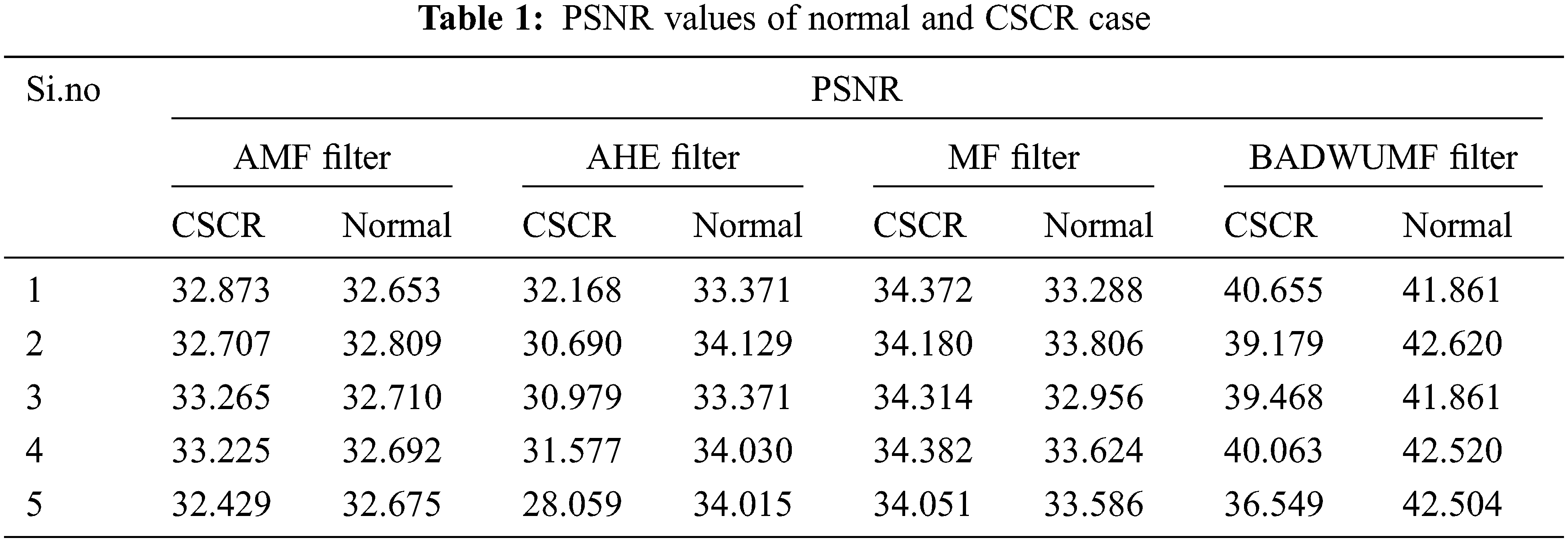
For performance analysis, four different parameters are considered they are Peak signal to Noise Ratio (PSNR), Structural Similarity Index Measure (SSIM) , Mean Square Error (MSE) and Signal to Noise Ratio (SNR). These performance evaluations metrics are calculated from every preprocessed image of retinal OCT database samples. Finally, their values are tabulated such as Normal cases and CSCR cases. Tab. 1 displays the PSNR values of the normal and CSCR case of the retinal database sample image. For analysis, in each case, only 5 samples of OCT images are taken. From the table known, the proposed BADWUMF method gives a PSNR value is 42.620 for normal retinal OCT sample 2 image and 40.655 for CSCR OCT retinal sample 1 image. This method provides better PSNR values when compared to AMF, AHE, and MF preprocessing methods.

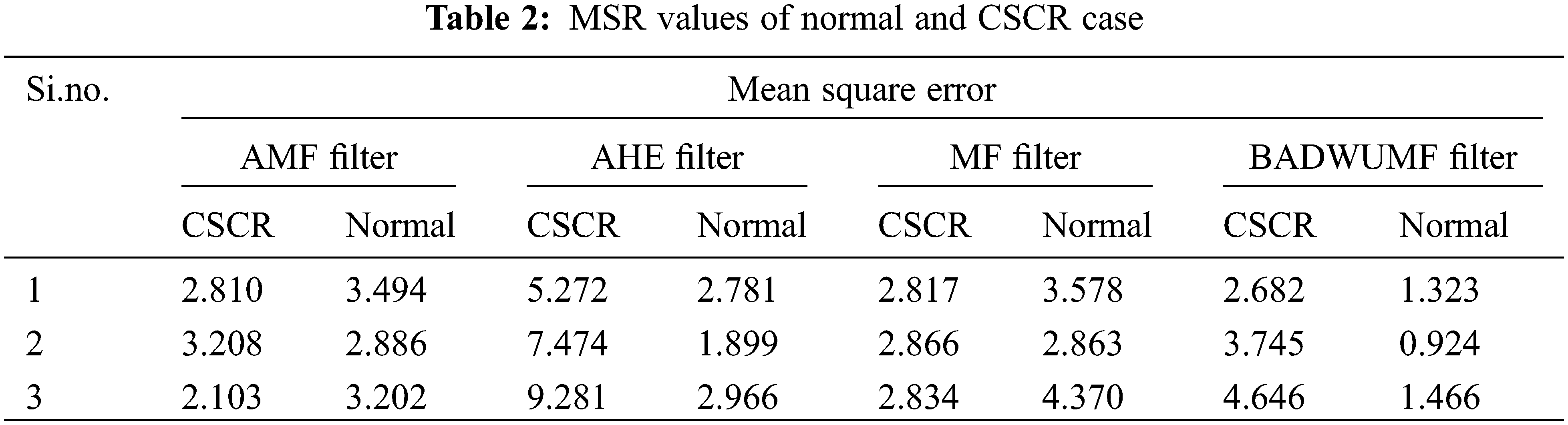
Tab. 2 shows the MSE values for AMF, AHE, MF and proposed BADWUMF preprocessing techniques in 5 images of CSCR and normal OCT samples. MSE value for the retinal OCT database sample is 0.988, 0.924 for BADWUMF, and 11.991 for the AHE method. The MSE is minimum as possible to prove the proposed technique is best among other preprocessing techniques.

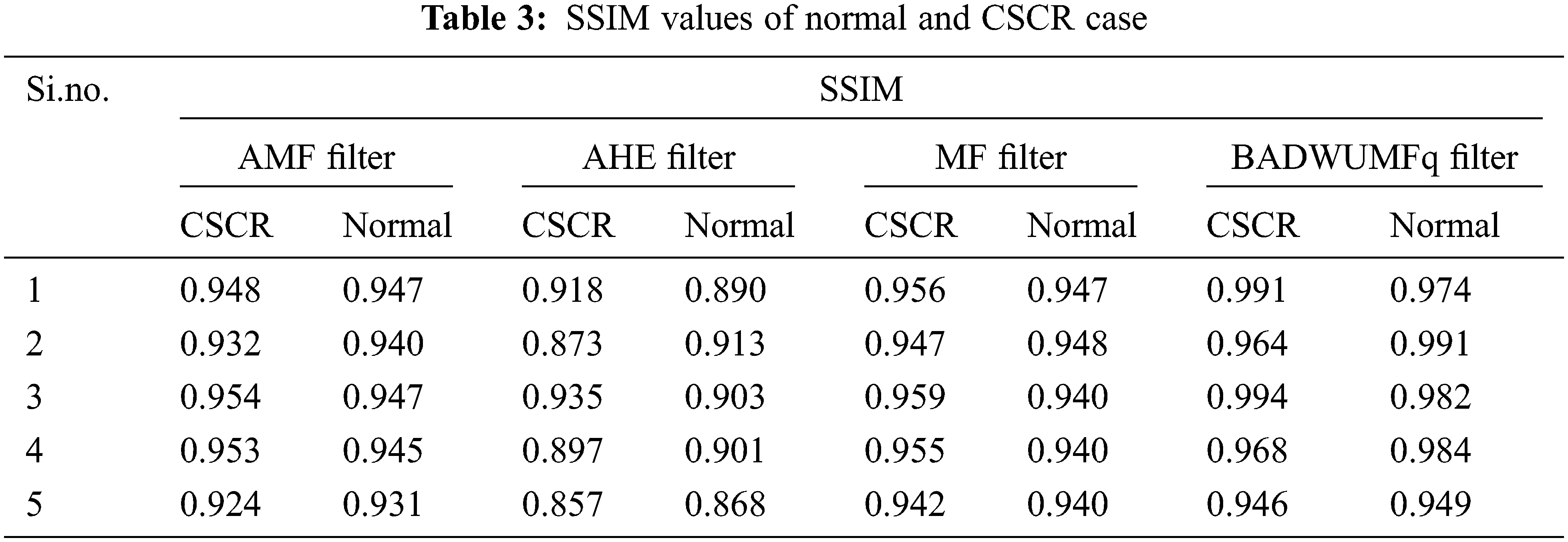
SSIM for various filters are shown in Tab. 3 for 5 images of CSCR and normal retinal database samples. SSIM value is maximum as possible to justify the proposed algorithm is better than other methods involved in the preprocessing stage. SSIM value is 0.991 for CSCR retinal OCT sample 1 and 0.991 for normal OCT retinal sample 2. SSIM value is 0.857 for the AHE method which is the least value given in the table for sample 5 CSCR retinal image.

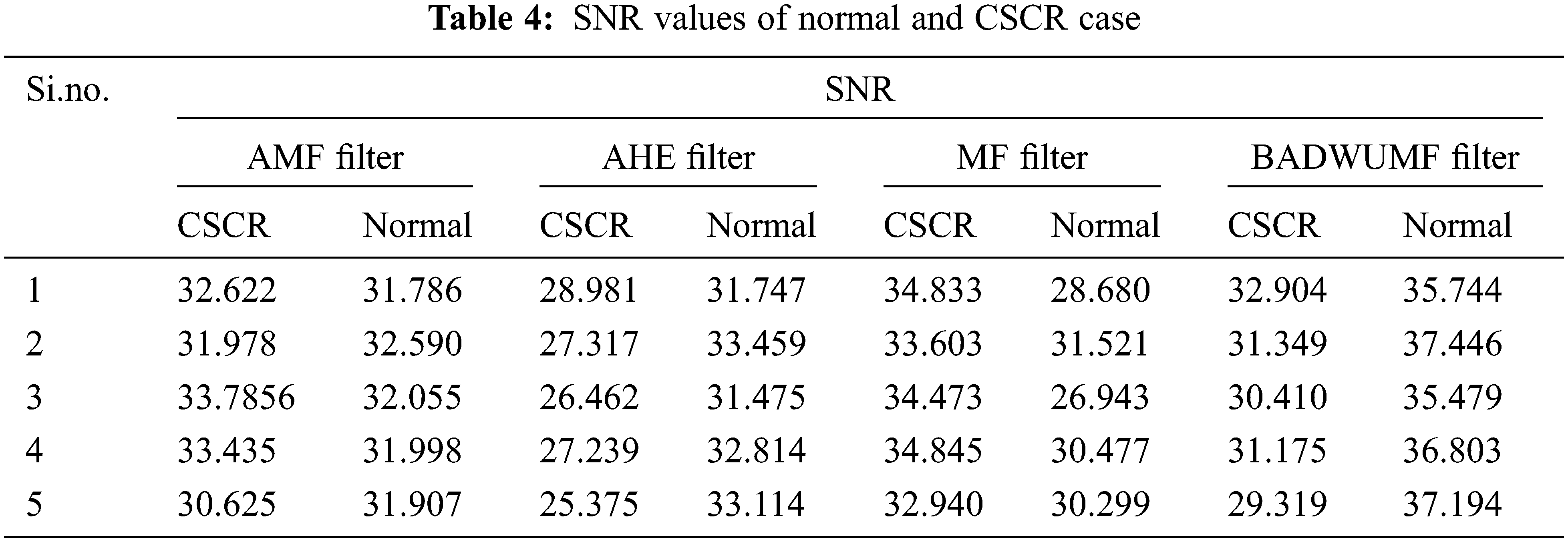
Tab. 4 shows the SNR values for AMF, AHE, MF, and proposed BADWUMF preprocessing techniques in 5 images of CSCR and normal retinal samples. The SNR value is maximum for proposed BADWUMF (37.446) than AHE (25.375) preprocessing method.

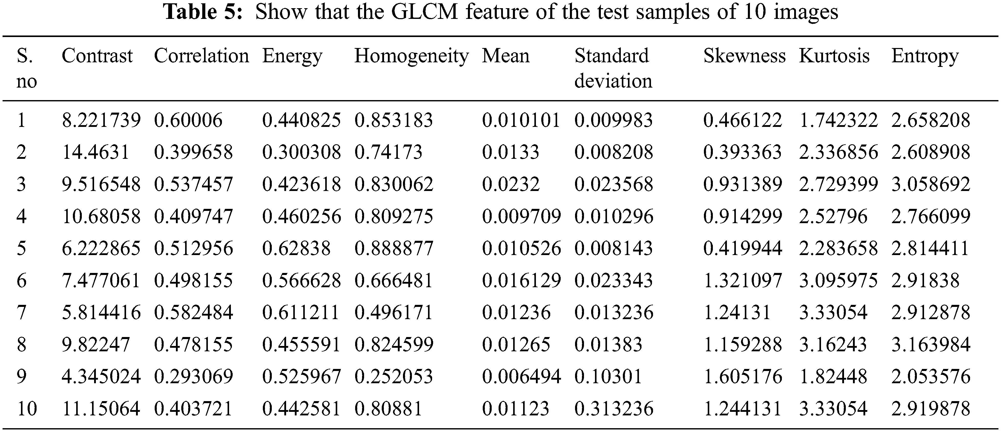
The GLCM function of 10 images in the test sample is seen in Tab. 5. It consists of 5 standard OCT and 5 CSCR OCT images. In Eqs. (8)–(16), the mathematical expressions are defined. These characteristics are taken from the pre-processed image. These characteristics are used as a classification reference.

Class 0 is seen in Fig. 5a as a standard OCT picture and Class 1. Of the overall 75 usual instances, 64 are correctly classified as normal True Positive (TP), with GLCM-related functionality, while 11 are incorrectly classified as CSCR False Negative (FN). 71 of the 75 CSCR test cases are categorized correctly as CSCR True Negative (TN), of which four are misclassified as usual False Positive (FP). Two class support vector machine uncertainty matrixes, a percentage TP of 42,7%, an FP of 11%, and FNs of 2.7%, and a TNs of 47,3%. The TCSVM rating is 90% accurate. 90%. The error rates are 10 percent. The Receiver Operating Characteristic (ROC) curve is shown in Fig. 5b

Figure 5: Classifier outputs obtained using two class support vector machine (TCSVM) (a) Confusion matrix (b) ROC curve

Class 1 displays regular OCT scanning image in Fig. 6a and class 2 shows CSCR OCT scanning image. 70 of the 75 overall normal cases are appropriately categorized as normal (TP) and 5 of those with GLCM related features are wrongly qualified as CSCR SNNWPB classifier (FN). Of the 75 CSCR cases evaluated, 70 are categorized correctly as CSCR (TN), of which 5 are misclassified as usual (FP). The percentage of uncertainty classifying SNNWPB is 46,7%, the percentage of FPs is 3,3%, the percentage of FNs is 3,3% and the % of FNs is 46,7%. The SNNWPB classification is correct at 93.3%. The misclassification figure is 6.7%. The Receiver Operating Characteristic (ROC) curve is shown in Fig. 6b.

Figure 6: Classifier outputs obtained using shallow neural network with powell-beale (SNNWPB) (a) Confusion matrix (b) ROC curve

From Tab. 6, the accuracy obtained using the SNNWPB classifier is 93.3% which is higher than that those obtained using TCSVM methods. The sensitivity and characteristics of the positive and negative labels are real. The error is 6.7% which is poor relative to the Classification TCSVM.

We also implemented a new clinical decision support system based on the OCT that can categorize normal OCT and CSCR OCT images. The proposed technique result showed that the SNNWPB classifiers are achieved better accuracy than the other forms of classification. SNNWPB classifier has achieved a 93.3% accuracy for classification which is greater than that achieves using TCSVM. Apart from this, the proposed approaches are useful in detecting the early stages of the CSCR case. We intend to prove that the proposed boosted anisotropic diffusion with an unsharp masking filter is used more reliable for the image enhancement process. This analysis is carried out on a laptop with an i7 processor from Intel core with the software MATLAB 2019. The method proposed is therefore helpful in classifying the CSCR images easily. The findings produced in this method indicate the proposed method has an adequate improvement and clinically identified the disorder. The suggested working approach thus becomes a brilliant solution for classifying OCT images and making them easy to view in hospitals. The device suggested also assists ophthalmologists in screening retinal patients in various geographical areas around the world. By training it on larger and comprehensive datasets, we will constantly improve the accuracy of the classifier in the future.

Acknowledgement: We show gratitude to anonymous referees for their useful ideas.

Conflicts of Interest: The authors declare that they have no conflicts of interest to report regarding the present study.

References

D. Pascolini and S. P. Mariotti, “Global estimates of visual impairment,” British Journal of Ophthalmology, vol. 96, no. 5, pp. 614–618, 2012.
M. Tang, “Image segmentation technology and its application in digital image processing,” in Int. Conf. on Advance in Ambient Computing and Intelligence (ICAACI), Ottawa, ON, Canada, pp. 158–160, 2020.
D. LoCastro, V. Cesare and T. Domenico, “Retinal image synthesis through the least action principle,” in IEEE 5th Int. Conf. on Intelligent Informatics and Biomedical Sciences (ICIIBMS), Okinawa, Japan, pp. 111–116, 2020.
R. Pallab, T. Ruwan, C. Khoa, D. M. Suman Sedai, M. Stefan et al., “A novel hybrid approach for severity assessment of diabetic retinopathy in colour fundus images,” in IEEE 14th Int. Symp. on Biomedical Imaging, Melbourne, VIC, Australia, pp. 1078–1082, 2017.
S. Muthuselvi and P. Prabhu, “Digital image processing techniques–A survey,” International Multidisciplinary Research Journal, vol. 5, no. 11, pp. 1–7, 2016.
Z. Gao, W. Bu, X. Wu and Y. Zheng, “Thickness measurements of ten intra-retinal layers from optical coherent tomography images using a super-pixels and manifold ranking approach,” in Int. Congress on Image and Signal Processing, BioMedical Engineering and Informatics (CISP-BMEI), Datong, China, pp. 1370–1375, 201
D. C. Fernández, H. M. Salinas and C. A. Puliafito, “Automated detection of retinal layer structures on optical coherence tomography images,” Optics Express, vol. 13, no. 25, pp. 10200–10216, 2005.
A. M. Bagci, M. Shahidi, R. Ansari, M. Blair, N. P. Blair et al., “Thickness profiles of retinal layers by optical coherence tomography image segmentation,” American Journal of Ophthalmology, vol. 146, no. 5, pp. 679–687, 200
P. V. Sudeep, S. I. Niwas, P. Palanisamy, J. Rajan, Y. Xiaojun et al., “Enhancement and bias removal of optical coherence tomography images: An iterative approach with adaptive bilateral filtering,” Computers in Biology and Medicine, vol. 71, no. 4, pp. 97–107, 2016.
N. H. B. Ismail, S. D. Chen, L. S. Ng and A. R. Ramli, “An analysis of image quality assessment algorithm to detect the presence of unnatural contrast enhancement,” Journal of Theoretical and Applied Information Technology, vol. 83, no. 3, pp. 415–422, 2016.
R. S. Choras, “Image feature extraction techniques and their applications for CBIR and biometrics systems,” International Journal of Biology and Biomedical Engineering, vol. 1, no. 1, pp. 6–16, 2007.
D. Puspita and A. N. Sigappi, “Detection and recognition of diabetic macular edema from OCT images based on local feature extractor,” International Journal of Pure and Applied Mathematics, vol. 119, no. 12, pp. 1–8, 2018.
L. Zhang, W. Zhu, F. Shi, H. Chen and X. Chen, “Automated segmentation of intraretinal cystoid macular edema for retinal 3D OCT images with macular hole,” in IEEE 12th Int. Symp. on Biomedical Imaging (ISBI), Brooklyn, NY, USA, pp. 1494–1497, 2015.
A. Roy, D. Dutta, P. Bhattacharya and S. Choudhury, “Filter and fuzzy c means based feature extraction and classification of diabetic retinopathy using support vector machines,” in Int. Conf. on Communication and Signal Processing (ICCSP), Chennai, India, pp. 1844–1848, 2017.
A. Rashno, D. D. Koozekanani, P. M. Drayna, B. Nazari, S. Sadri et al., “Fully-automated segmentation of fluid/Cyst regions in optical coherence tomography images with diabetic macular edema using neutrosophic sets and graph algorithms,” IEEE Transaction on Biomedical Imaging, vol. 65, no. 5, pp. 989–1001, 2017.
S. Lee, N. Charon, B. Charlier, K. Popuri, E. Lebed et al., “Atlas-based shape analysis and classification of retinal optical coherence tomography images using the functional shape (fshape) framework,” Medical Image Analysis, vol. 35, no. 1, pp. 570–581, 2017.
R. Rasti, H. Rabbani, A. Mehridehnavi and F. Hajizadeh, “Macular OCT classification using a multi-scale convolutional neural network ensemble,” IEEE Transactions on Medical Imaging, vol. 37, no. 4, pp. 1024–1034, 2018.
D. Xiang, G. Chen, F. Shi, W. Zhu, Q. Liu et al., “Automatic retinal layer segmentation of OCT images with central serous retinopathy,” IEEE Journal of Biomedical and Health Informatics, vol. 23, no. 1, pp. 283–295, 20
S. Ravishankar, A. Jain and A. Mittal, “Automated feature extraction for early detection of diabetic retinopathy in fundus images,” in IEEE Conf. on Computer Vision and Pattern Recognition, Miami, FL, USA, pp. 210–217, 2009.
Z. Yavuz and C. Köse, “Blood vessel segmentation from retinal images based on enhencement methods,” in 22nd Signal Processing and Communications Applications Conf. (SIU), Trabzon, Turkey, pp. 907–910, 2014.
Z. Wang, M. W. Jenkins, G. C. Linderman, H. G. Bezerra, Y. Fujino et al., “3-D stent detection in intravascular OCT using a Bayesian network and graph search,” IEEE Transactions on Medical Imaging, vol. 34, no. 7, pp. 1549–1561, 2015.

Computer Systems Science & Engineering DOI:10.32604/csse.2023.024449
Article