DOI:10.32604/csse.2023.025166
| Computer Systems Science & Engineering DOI:10.32604/csse.2023.025166 | |
| Article |
Container Based Nomadic Vehicular Cloud Using Cell Transmission Model
1Department of Computer Science and Engineering, Jayam College of Engineering and Technology, Dharmapuri, 636813, India
2Department of Electronics and Communication Engineering, Adhiyaman College of Engineering, Hosur, 635109, India
*Corresponding Author: Devakirubai Navulkumar. Email: flytondk@gmail.com
Received: 14 November 2021; Accepted: 07 January 2022
Abstract: Nomadic Vehicular Cloud (NVC) is envisaged in this work. The predominant aspects of NVC is, it moves along with the vehicle that initiates it and functions only with the resources of moving vehicles on the heavy traffic road without relying on any of the static infrastructure and NVC decides the initiation time of container migration using cell transmission model (CTM). Containers are used in the place of Virtual Machines (VM), as containers’ features are very apt to NVC’s dynamic environment. The specifications of 5G NR V2X PC5 interface are applied to NVC, for the feature of not relying on the network coverage. Nowadays, the peak traffic on the road and the bottlenecks due to it are inevitable, which are seen here as the benefits for VC in terms of resource availability and residual in-network time. The speed range of high-end vehicles poses the issue of dis-connectivity among VC participants, that results the container migration failure. As the entire VC participants are on the move, to maintain proximity of the containers hosted by them, estimating their movements plays a vital role. To infer the vehicle movements on the road stretch and initiate the container migration prior enough to avoid the migration failure due to vehicles dynamicity, this paper proposes to apply the CTM to the container based and 5G NR V2X enabled NVC. The simulation results show that there is a significant increase in the success rate of vehicular cloud in terms of successful container migrations.
Keywords: Vehicular cloud; container migration; cell transmission model; 5G NR V2X PC5 interface
Static [1–3] and dynamic [4,5] VC are classified according to the movement of the vehicles participating in VC. Static VC is so named because the vehicles involved are ‘static’ in one location (like a parking lot). In practice, even static vehicles may leave their location at any moment, necessitating the same resource volatility management as dynamic VC [1]. The sole distinction is that dynamic VC has a very high level of resource volatility, while static VC has a very low level of resource volatility. As a result, this work considers both static and dynamic VC in terms of VC movement. Static VCs operate in a specific place, such as around a base station, with moving or parked cars, or both, while dynamic VCs operate with moving vehicles on the road and move in parallel with the VC initiator. It’s worth mentioning that, while studies suggest VC based on vehicle movement, there are only a few research that address VC moving along with a vehicle. The objective of this work is to create a 5G NR V2X PC5 enabled VC that only uses vehicle resources and it move along with a vehicle that initiates the VC.
Establishing and sustaining Vehicular Cloud (VC) [4–7] is the demanding step of VC implementation. Owing to the rapid mobility design of the vehicles, the connection between the VC members is very fluctuating and in turn, the efficiency of VC is reduced. This work focus to build a reliable NVC with the maximum stabilised topology. To accomplish this, the proposed VC is built only with the resources of moving vehicles on the highway without using any additional infrastructures and an efficient mechanism is constructed to determine the container (task) migration initiation time within VC. The motivational features of 5G NR V2X [8] are the reason for choosing NR V2X for NVC implementation. The new transmission types, unicast and groupcast help to communicate within NVC and finally the advanced security features justify the use of NR V2X for NVC. 5G New Radio Vehicle-to-Everything (NR V2X) Mode 2(a) is used in this work because of its enhanced features than the Cellular V2X (C-V2X) mode 4 [9], as it is specially designed for V2V communications using PC5 sidelink interface without relying on the cellular infrastructure support.
Cooperative Awareness Message (CAM) [10] and Decentralized Environmental Notification Message (DENM) [10] are the two message forms that floats between vehicles using direct communication mode. In the proposed work, to avoid transacting additional messages, CAM and DENM are used to create NVC. VM and its migration are the baseline of vehicular cloud. Each service, like Infrastructure as a Service (IaaS), Platform as a Service (PaaS) and software as a service (SaaS) has a different focus, but all have VM migration as an underlying operation [11]. This work uses Containers in the place of VMs. Containers are more light weight and use fewer resources than VMs [12]. Containers have too short life cycle than VMs and more dynamic in use. It takes less time to implement, operate, and monitor. Containers are much more mobile than VMs because they can launch and run applications within seconds. Similar to the reason for VM migration, container migration is necessary to face the dynamic nature of VC. Container migration has a significant role in VC and also it is the major challenge for VC. The main contribution of this work is to address the unsuccessful container migrations due to dual mobility of VC participants by applying CTM [13] to the proposed NVC. Therefore, it is intended to mitigate the failure rate of NVC due to container migration failure to increase the reliability of NVC.
Distance and coverage area are the two factors that leads a vehicle to discontinue its participation from the vehicular cloud. When the distance between the VCI and VCM increases, the PC5 interface connection begins to fade out and the undergoing process gets interrupted. To preserve the proximity between VCI and VCM, it is important to determine when and where to migrate the container in a VCM whose distance from the VCI is expected to be above the limit. This decision on container migration is facilitated by applying CTM. CTM is used to simulate the actual traffic state of a road. This model estimates the position and number of vehicles in each section of the road. As the traffic conditions are simulated the motions of VCI and VCMs can be predicted. So prior decision making about the containers of the exiting VCM can be attained.
The rest of the paper is organized as follows. Section 2 discusses about the concepts of vehicular cloud, sidelink interface, container migration and CTM. Nomadic Vehicular Cloud is introduced in Section 3. The performance of NVC is evaluated using simulation in Section 4 and concluded in Section 5.
Vehicular Cloud is intriguing due to the unused resources in contemporary automobiles. Mobility of vehicles involving in VC, communication model applied to VC, the choice of VM or containers, vehicle residency time within VC are the major factors that decides the performance of VC. The primary aspect of VC, as well as its primary obstacle, is the mobility of vehicles. As a result, comparatively, few articles on VCs focused on the parked automobiles [1–3] and few others experimented into datacenters made from automobiles parked at a large parking lots. The distinguishing between static and dynamic VC is made primarily on resource volatility caused by vehicle speed rather than network connectivity [5].
Dynamic VC [5], which works with moving cars on highways and access points that have been pre-installed. Access points are linked to the VC controller. The extension of [5] includes job migration, whereas each job is encapsulated as container images [4]. References [6,14] proposes VC with wireless base stations as data hosts. Wireless base stations [6] act as the initiator of VC and VC is static in the area around the wireless base station. Vehicles entering the region participate in the VC with their own choice and interest. The ongoing workload of the vehicles departing from the region has been migrated to other vehicles within the region. Conventional edge clouds [14] offload computing processes to VC, proposed Cooperative task scheduling scheme for VC and developed a vehicular mobility model to increase the vehicular residency time of the vehicles involving in VC. Connected vehicular cloud computing (CVCC) [15] technology is a hybrid VC that exploited the resources in the internet cloud, RSUs and vehicles. The internet cloud and RSUs serve as the main computation service provider for vehicles. Out sourcing concept is introduced in CVCC, the vehicle that receives the task can outsource sub-task to other vehicles.
Reference [16] explored with ways to improve VC’s reliability and availability in terms of vehicle residency time. To extend the vehicle residency duration, they developed redundancy-based work assignment methodologies. Their method extends the duration of a vehicle’s stay, which has the unintended consequence of increasing resource use. Vehicle residency time is treated as the cell residency time [14] of vehicles since they are in the VC as long as they are inside the coverage of the base station and simulated using the Hyper-Erlang distribution [17].
The communication model applied to the VC have an impact on the performance of the VC. In Reference [4,5,16], DSRC (Dedicated Short Range Communication) is applied to VC. When compared to the 5G NR V2X PC5 interface, DSRC has a lower data transfer rate, shorter communication range [18] and lower Packet Reception Ratio [19]. Reference [20] discuss about the PC5 QoS model for NR sidelink, group cast and unicast V2X communication connection establishment and the physical layer design of the NR side link as per 3GPP Release 16. The evolution of V2X standards [21–25] towards IEEE 802.11bd paves way to double the IEEE 802.11p communication range, up to 1000 m. The 5G NR V2X’s goal is to support extended sensor applications that require high bandwidth to communicate huge quantity of data [20].
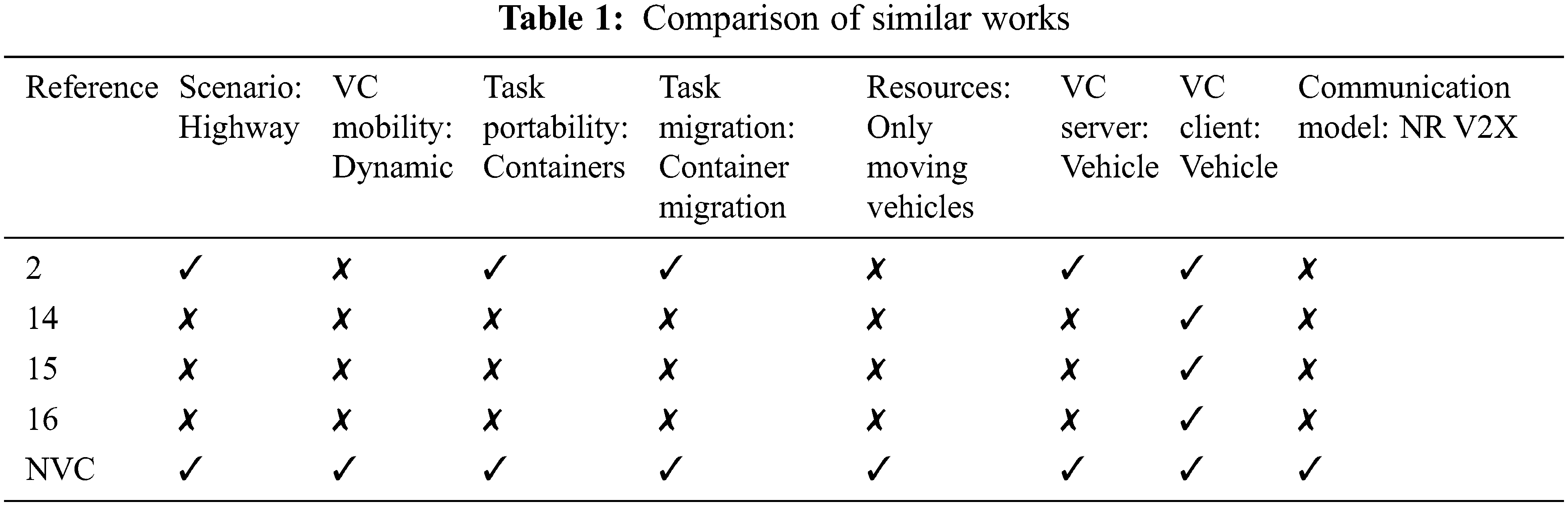
The efficient migration of VM or containers plays a key role in VC, as in the traditional cloud. The initiation time of the container migration process is one aspect that determines the performance of the migration process. Reference [6] handled this problem in the term ‘first hop’ failure. The traffic density in the chosen scenario is an another important factor of VC. Higher traffic density and logically partitioning the road helps the migration process to be successful [13,22]. The length of the road segment is measured on the basis of the length of the vehicle travelling for a given time [13]. Tab. 1 compares the related work. CTM [13] is used in this work to decide the time for container migration on the basis of their concept of road segmentation. Basically, by measuring the traffic density and traffic flow at specific locations at different stages of time, CTM predicts the traffic attitude on the identified road stretch. A key requirement for VC to avoid dis-connectivity among its participants is to estimate the spatio-temporal data of vehicles. By applying CTM to VC, the movements of vehicles can be calculated and the start time of the container migration can be calculated using it. To the best of our understanding, this is the first effort to apply CTM concept in VC to determine the time to initiate the container migration.
A container based Nomadic Vehicular Cloud (NVC) using CTM is proposed here. The moving vehicles on the road are NVC participants. In contrast with [2,6], NVC is initiated by one of the moving vehicles on the road. The NVC region moves along with the vehicle that initiated the NVC. Vehicles moving around the initiator are selected as VC members.
3.1.1 Establishing Nomadic Vehicular Cloud
NVC uses 5G V2X PC5 interface to build the vehicular cloud. NVC communicates in the range of 1000 m [23]. VCI, searches for the potential moving vehicles that can act as a VCM. VCI, through CAM beacons, broadcasts the VC member request to the single hop vehicles. Vehicles that receive the CAM beacons, if it has the requested resources with the required resource capacity and time, triggers DENM transmission that consists of the information about the resources and its capacity. VCI forms a resource profile registry from the collected DENMs. VCI selects the VCMs from the resource profile registry to create the Vehicular Cloud. By using periodic CAMs and event-triggered DENMs, the resource profile registry is periodically updated. When one of the following events happen in the environment, the resource profile registery is modified using CAMs even after the VC is established: (i) a new vehicle enters into the range, (ii) one of the VCMs leaves the range and (iii) when any of the VCM complete its task while it is within the range.
3.1.2 NVC in Cell Transmission Model
Heavy traffic environment of the road is considered and exploited for this work. The peak traffic provides the opportunity to utilize the resources of many vehicles, but the mobility of vehicles tends to raise the problem of dis connectivity between NVC participants. This issue is handled with the aid of CTM. Prior estimation of vehicle movement and initiating the container migration process at the earliest are the aim of applying CTM to NVC. The pre informed container migration initiation, increases the success rate of container migration across NVC. The container migration time remains same [24], as it is assumed that the containers’ size are fixed and the bandwidth are same between VCMs. In the proposed work, each VCM receives containers in different size and hence the container migration time differs. The rate of container migration requirement to maintain the VC topology, found very low with the combination of establishing NVC with CTM in a heavy traffic road.
3.1.3 Container Migration in NVC
Container migration is one of the key factor that decides the reliability and availability of Vehicular Clouds. When the VCMs drive at the same speed without accelerating or decelerating, at a given point of time, the containers are either migrating its workload from VCI to VCM or perform its task at VCM or migrate the result back to the VCI from VCM. While containers performing its task at VCM, due to the speed variance of vehicles, VCMs may leave out of the coverage of VCI. To avoid this, before leaving the coverage of VCI, VCMs need to migrate its containers to another VCMs within the coverage of VCI. To make decision on when and where to migrate the container, in the CTM applied NVC environment, a time and space dependent procedure is implemented. The intention of applying CTM to NVC is to complete the container migration process before the VCM leaves the coverage area of VCI.
There can be a failure in either of the above steps while container migration. If the container failed to migrate back to the VCI, the failed state would persist indefinitely and it is called as a non-recoverable state. For a period of time, a recoverable condition will continue in the broken state until the unfinished container is reassigned to the other possible vehicle and the incomplete job is done. The non-recoverable state is a condition at t and have a constant failure rate, if either the container with incomplete task cannot be assigned to any other vehicle or if the container migrates back to VCI gets interrupted.
CTM [13] is used to simulate the time based actual traffic conditions for a defined stretch of road. The established VC in the 1 Km range is framed into CTM. The notations used are summarized as following, S as Segment set, ns as Number of segments, nrs as Number of segments in Range,
Among all the vehicles flowing into CTM, vehicles agreed to act as a VCM are labelled with M and VCI is labelled with I. The defined stretch of road where NVC is to be established, is parted into segments,
Since the vehicles are on the move, while establishing and maintaining VC, the position of range segments on the road differ for every time step. Though the range distance is 1 km, physically this 1 km distance varies on the road. For example, if 15 segments are assumed, the segments in the range are 1, 2 & 3 for the first time step, the segment in the range becomes 2, 3 & 4 for the second time step, etc. Hence, for the proposed work, simulation is carried out for 5 times the number of segments. The maximum number of vehicles in a segment at a time step is evaluated with the bottleneck density and Sd.
To demonstrate the real traffic condition, the road stretch is considered with Bottleneck Situations (BS) in varying time duration. BS induces on-the-road congestion. With the high congestion level, vehicles’ speed is decreased. This forced the VC vehicles to stay with in the Range of Segments (ROS) for an extended period of time. The movement of vehicles into segments therefore depends on the density of vehicles that varies during the flow of bottleneck traffic, BF, and ordinary traffic flow, NF. θN and θC can be approximated with the assumed BF and NF. ΔR, the maximum number of vehicles that can flow in the given road stretch per hour is assumed (3000 veh/hr) based on the road conditions. With ΔR,
In a normal traffic flow, it is presumed that all vehicles in a segment proceed to the next segment for each time step, ts,
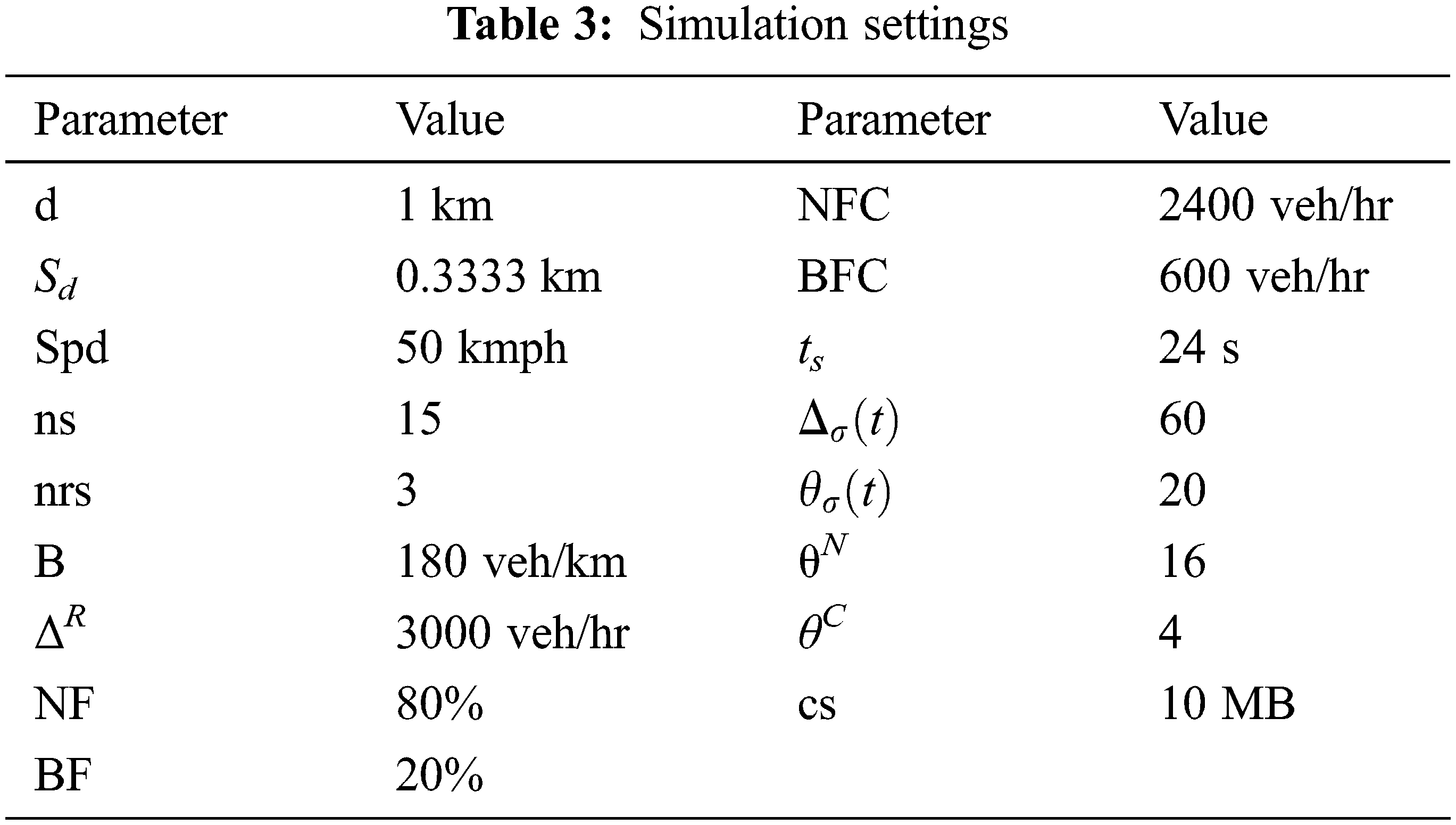
A traffic entry table [13] is generated with the values of the equations Eqs. (1)–(6) as constants and the value of Eq. (7) as the occupancy of each segment at t. The entries in the traffic flow entry table are as seen in Tab. 3. Here,
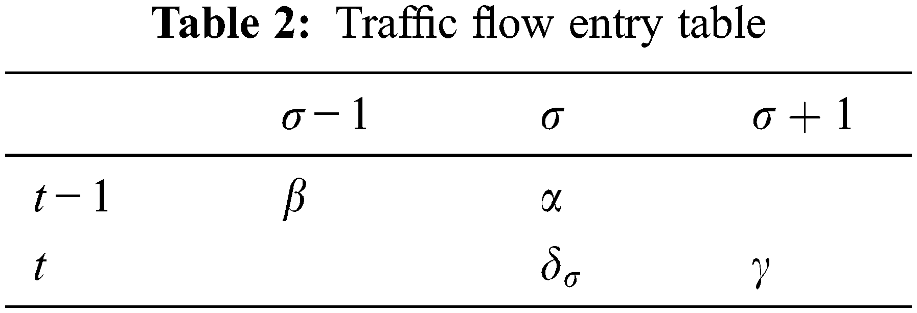
When a vehicle from
By applying CTM to NVC, VCI is identified as σVυ I and VCMs can be identified as σ − 1Vυ M, σVυ M, σ + 1Vυ M. Algorithm 1, presents the pseudocode that frames the NVC environment in CTM. In practical, vehicles speed can wave up to the road speed limit. Therefore vehicles can keep moving to next cells or it can slow down in the same cell for a specific period. This speed variation can lead the NVC participants to get disconnected from the NVC. This instance raises the requirement to focus on maintaining proximity between VCI and VCM. The position of the containers in the VCM’s within VC can be tuned based on the VCI ‘s position.
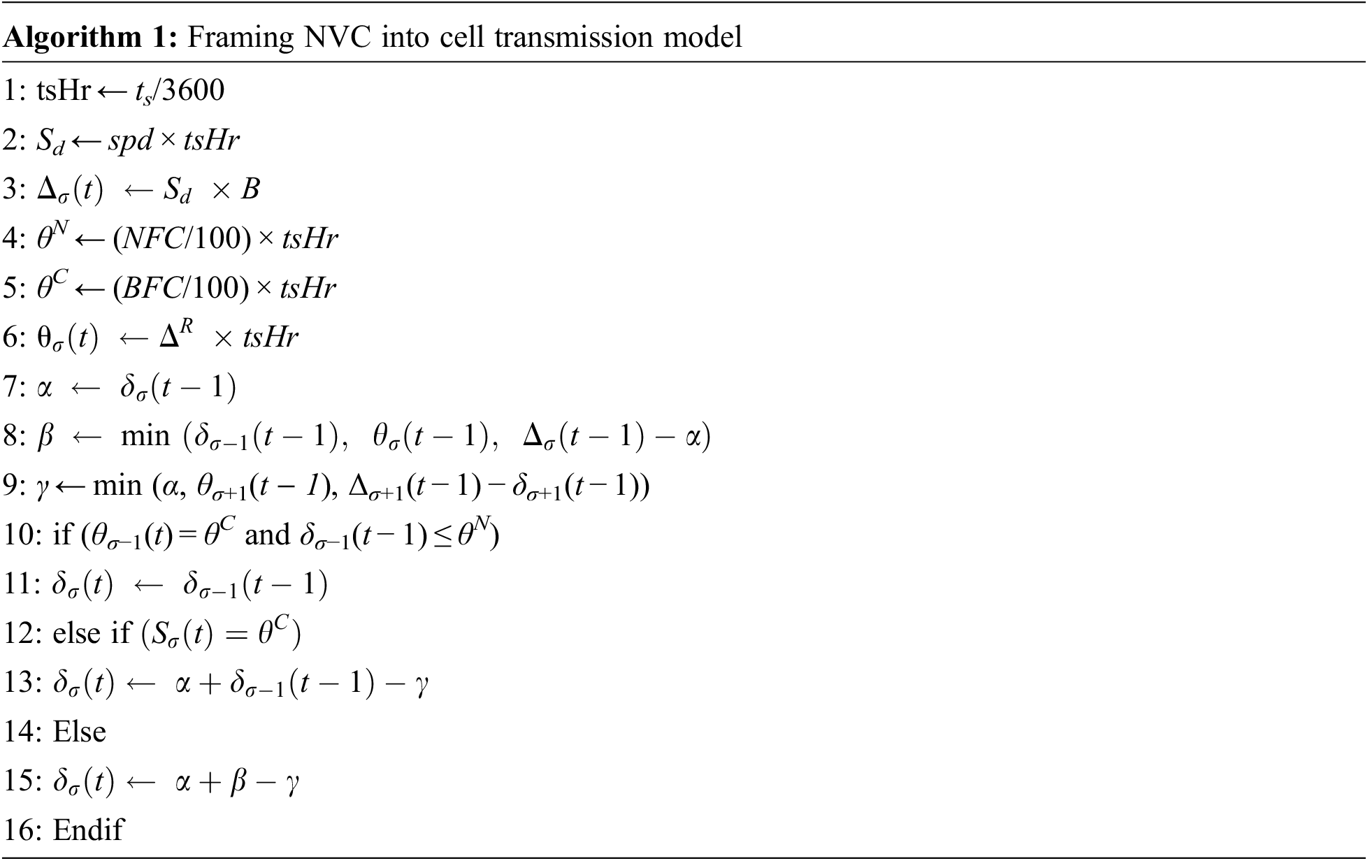
Vehicle speed spd is assumed as constant, so vehicles flow in same speed until a bottleneck situation (BS) occurs on the way of VC. Therefore, vehicles’ acceleration can be decreased or sustained based on the occurrence of BS. VCI checks for BS within its range at each time step, in Sσ+2(t), Sσ+1(t) and
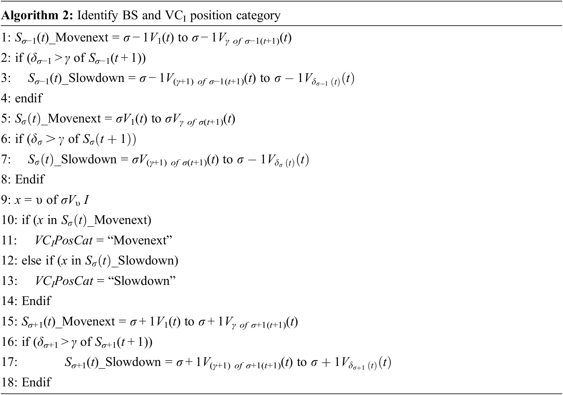
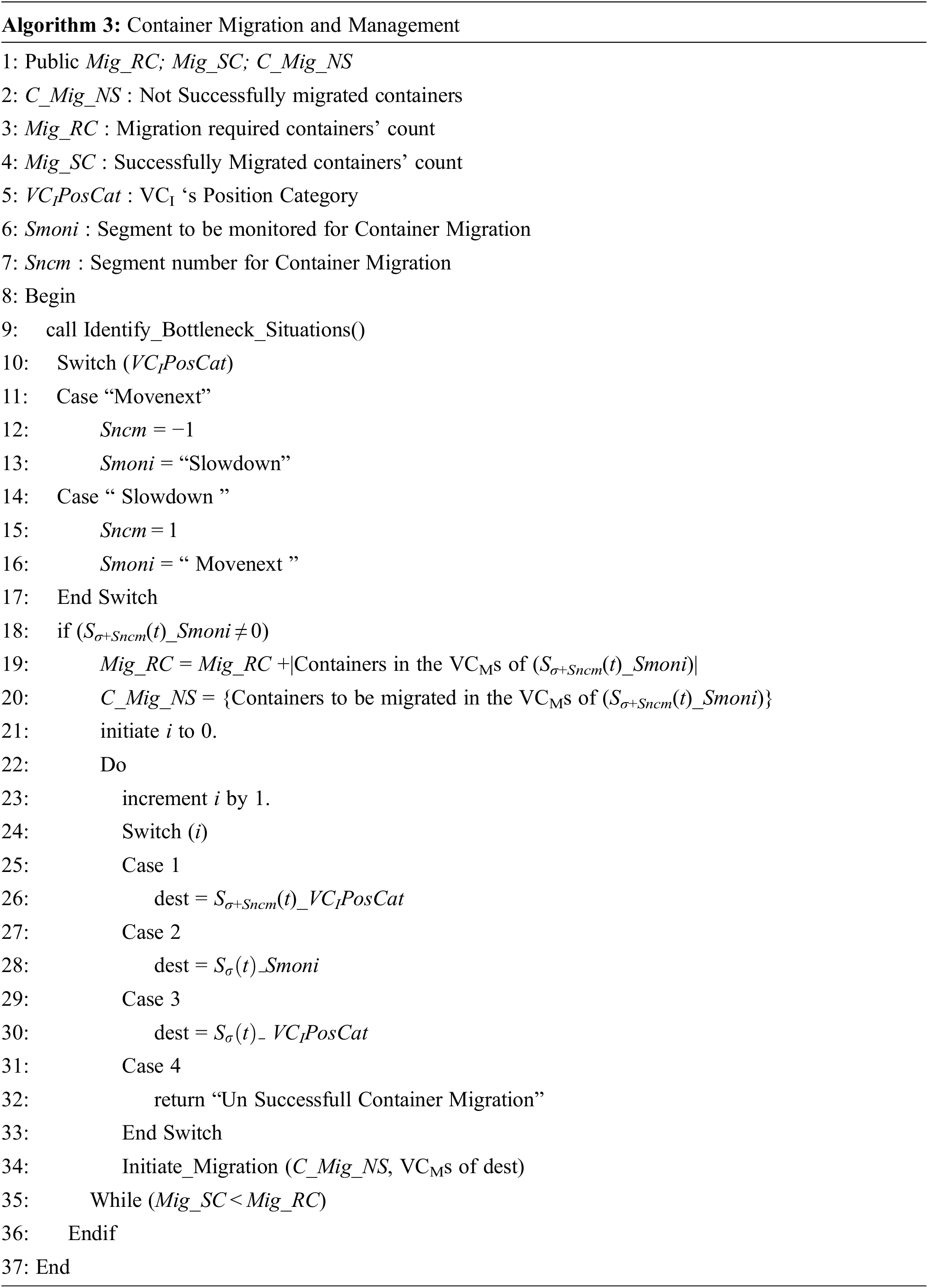
Migration decision is based on the position of VCI in
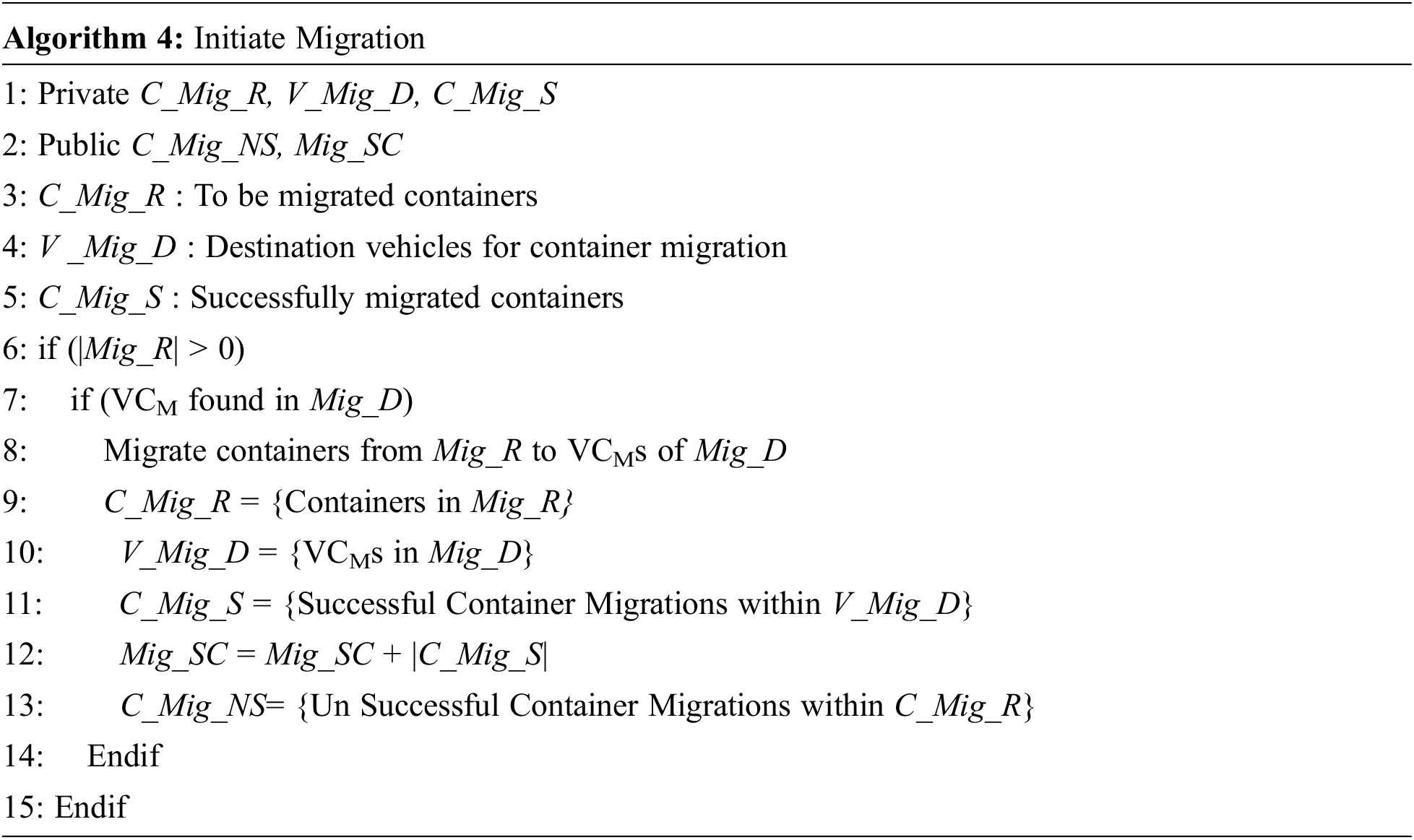
As coded in Algorithm 4, migration is initiated with two parameters, containers to be migrated and the destination vehicles’ range. With the assumption that no other overhead parameters are taken into account in this work, each container to be migrated is moved to the chosen destination, after finding the destination for migration. Predicting the percentage of vehicles in a particular segment S at time t helps to estimate the movement of VC participants with in CTM. This prediction is done using conditional probability mass function. Let T and X be the discrete random variables and [T,X] be a discrete random vector. X = x is being informed, where x is the realization of X. The conditional probability mass function of T given X = x is a function. PT|X→x: RTX → Ω, RT → ΩT where RTX and RT is the support vector and, Ω and ΩT are the sample spaces. Here,
To derive the probability mass function of T lets compute the marginal probability mass function of S by iteratively adding the joint probability mass over the support of RT. Let the joint probability mass function T be
Simulation using MATLAB was performed to test the efficiency of the proposed model, with the metrics to be observed.
The model built on MATLAB includes many modules. The road mobility model is built in SUMO. NVC is established with the formal request-reply model using V2X’s basic safety messages. The established NVC is framed in to CTM. A pre-informed migration decision algorithm is used to achieve the NVC task successfully. The simulation settings with the data are given in Tab. 3.
The rate of successful container migration and the rate of container migration requirement are the two metrics used to evaluate the proposed methodology. Only the dis connectivity of NVC participant due to high mobility is considered and assumed that the other metrics like enough resource space and the workload of the destination are well satisfied. The distance and time of VCM and VCI are used to gauge the success of container migration.
The proposed model was initially simulated without any bottlenecks when testing the metrics. The vehicle movement flows smoothly without any need for container migration, as the vehicle speed is constant. The bottleneck situations on the VC trajectory were later added. For the following scenarios, calculations will be carried out:
4.3.1 Scenario I-Bottleneck Situations (BS) in the Various Part of Range of Segments (ROS) at t + 1 with Three Distinct Traffic Flows at t
The various traffic flow trends considered in this scenario are, Free flow in all the segments of ROS (F), Congestion only in
When there exists a BS at the initial part of ROS, Sσ+1(t + 1), then each VCM in segment Sσ+1(t) is supposed to move to either Sσ+2(t + 1) or to Sσ+1(t + 1). Due to BS at Sσ+2(t + 1), only the assumed bottleneck flow percentage of vehicles can pass into Sσ+2(t + 1), and the remaining will be slowdown in Sσ+1(t + 1). While BS exists at the last part of ROS,
I. The destination selection for the migration of each container in VCMs of Sσ+1(t)_Movenext category is performed among the VCMs of Sσ+1(t) and
II. The destination selection for the migration of each container in VCMs of Sσ−1(t)_Slowdown category is performed among the VCMs of Sσ−1(t) and
4.3.2 Scenario II-Bottleneck Situations (BS) in Different Proximity
The different proximities are categorized as Initial segments-Earlier ts, Mid segments-Mid ts, Last segments-Last ts. The category of proximity is further parted into segments as First part : Sσ−1, Mid part :
4.3.3 Scenario III-the Occurrence Time of Bottleneck Situations
The BS occurrence time is categorized as Single ts, Double ts, triple and above ts. To simulate the impact of BS duration on the trajectory of VC, BS are assumed on the path of VC for single ts, double ts and triple and above ts in the same environment of scenario II.
Simulation was conducted by applying the settings and metrics at various phases as proposed in the previous sections. Each phase was simulated for 10 times and the results collected were averaged. The following subsections discusses about each phase of simulation with the given settings and metrics.:
4.4.1 Rate of Successful Container Migration (SCM) Based on the Impact of Bottleneck Situations (BS), in Different Part of ROS
Based on the simulations conducted, it is summarized that, regardless of the occurrence of BS in different part of ROS, container migration is not required in the following cases:
i) When there is a free traffic flow at ts and BS at the initial part of ROS at (t + 1)
ii) When there is a free flow at ts and VCI positions at
iii) When there is congestion only in
Among the following container migration requiring cases, case (i) and (ii) are due to the occurrence of BS, case (iii) is partially due to the occurrence of BS and other cases of migrations are required regardless of the occurrence of BS.
i) When there is a free traffic flow at ts and BS at the last part of ROS at (t + 1),
ii) When there is a free flow at ts and VCI positions at
iii) When there is congestion only in
iv) When there is congestion only in
v) When there is congestion in all segments of ROS at ts and BS in anywhere in initial, mid and last part of ROS at (t + 1).
For the above cases of required container migrations, item (i) requires |containers in Sσ−1(t)_Slowdown| number of container migrations, item (ii) and (iv) requires |containers in Sσ+1(t)_Movenext| and item (iii) and (v) requires |containers in Sσ+1(t)_Movenext| or |containers in Sσ−1(t)_Slowdown|. For the migration requirements of containers in Sσ+1(t)_Movenext, the destinations are VCMs of Sσ+1(t)_Slowdown and
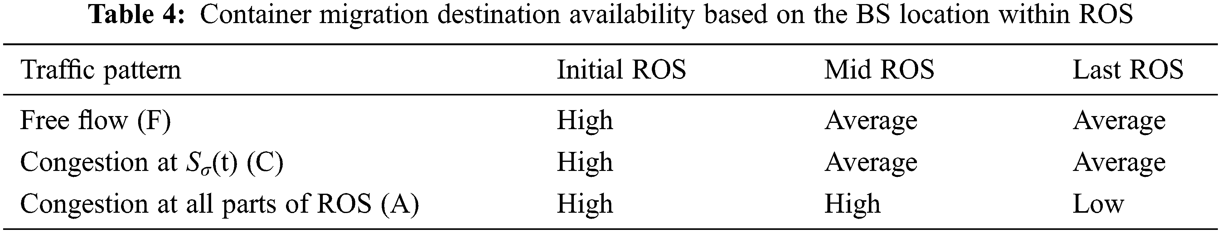
Fig. 1 illustrates the destination availability ratio of each case. The BS raises the container migration requirement in the following cases with average availability of container migration destinations: BS at mid part and last part of ROS with free traffic flow and congestion in all parts of ROS. Based on Fig. 1, the availability of container migration destination is classified in Tab. 4. Fig. 2 shows the rate of successful container migrations based on the impact of BS in various parts of ROS and different patterns of traffic flows. Whenever the container migration requirement is raised due to the occurrence of BS, the availability ratio is average, which in turn impacts the success rate of container migration within ROS. Comparing with the work of [6], where with the unrestricted resource usage and high congestion level, 97% of successful VM migration is achieved. In this work, with the unrestricted resource usage and high congestion in the entire ROS, the simulation results 98.8% of successful container migration.
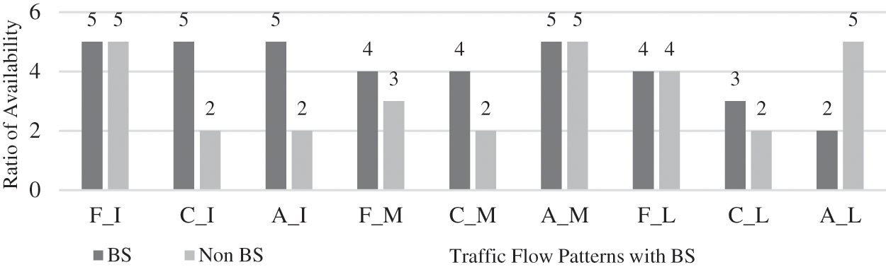
Figure 1: Ratio of destination availability for container migration
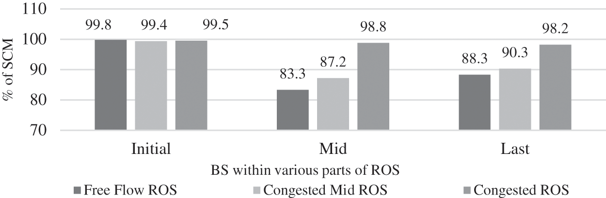
Figure 2: Ratio of SCM based on the impact of BS in various parts of ROS and different patterns of traffic flows
4.4.2 Rate of Successful Container Migration (SCM) Based on the Impact of BS Proximity on the Trajectory of VC
In the first part of the segments in each
The BS in the mid part of segments in each
There are |containers in Sx. (ts + i)_Movenext| number of container migration requirements, where i = 0 to t − 1, when BS occurs in a segment x that falls in to the ROS for t number of ts. The BS in mid part of segments at earlier ts in the first block of segments, have low rates of SCM, since the VC travels with a low number of vehicles within ROS. As showed in Fig. 3, the rate of SCM gradually increases in the second and third block of segments due to increase in the number of vehicles within the ROS as the BS happens during the later time steps. On the average, the impact of BS proximity on the trajectory of VC results 98.2% of SCM.
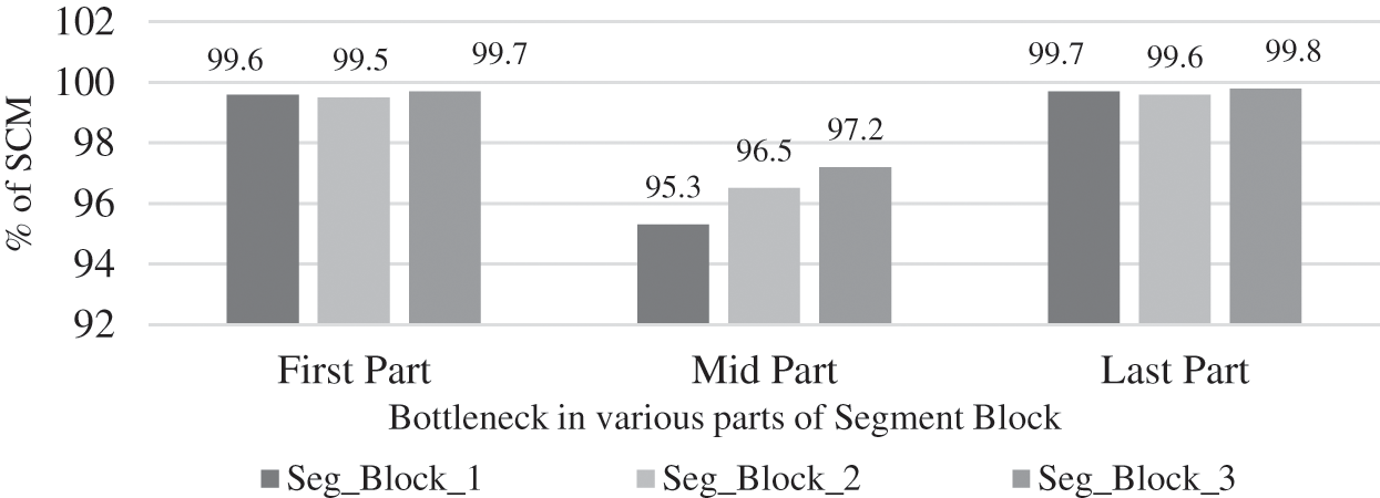
Figure 3: Ratio of SCM based on the effect of BS proximity on the trajectory of VC
4.4.3 Rate of Successful Container Migration (SCM) Based on the Impact of the Length of the BS on the VC Trajectory
If BS lost for a single ts in the first part of all the segment blocks, as in the other scenarios, completely have no impact. BS for single ts in the mid part of segment blocks, results comparatively high negative impact due to the less number of destinations for migration. This result is based on the VCI position and the container migration requirements raised due to it. In the last part of segment blocks, BS for triple and above ts has a positive impact as this case has a high number of destinations for migration. These facts are displayed in Fig. 4. While the same trend of the SCM rate follows in both double ts and single ts within the different parts of segment blocks, but as in Figs. 5 and 6, due to the reduction in the incidence period of BS, there is a steady decrease in the total SCM rate.
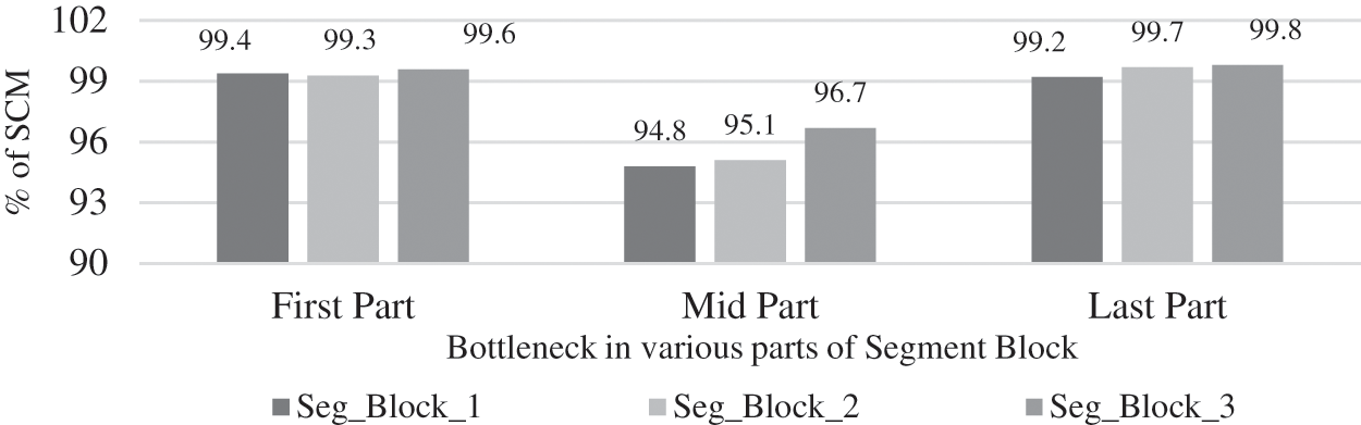
Figure 4: Ratio of SCM based on the impact of BS for triple and above time steps in various block of segments
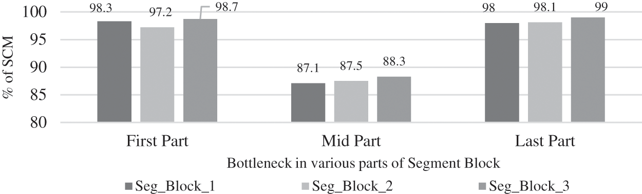
Figure 5: Ratio of SCM based on the impact of BS for double time steps in various block of segments
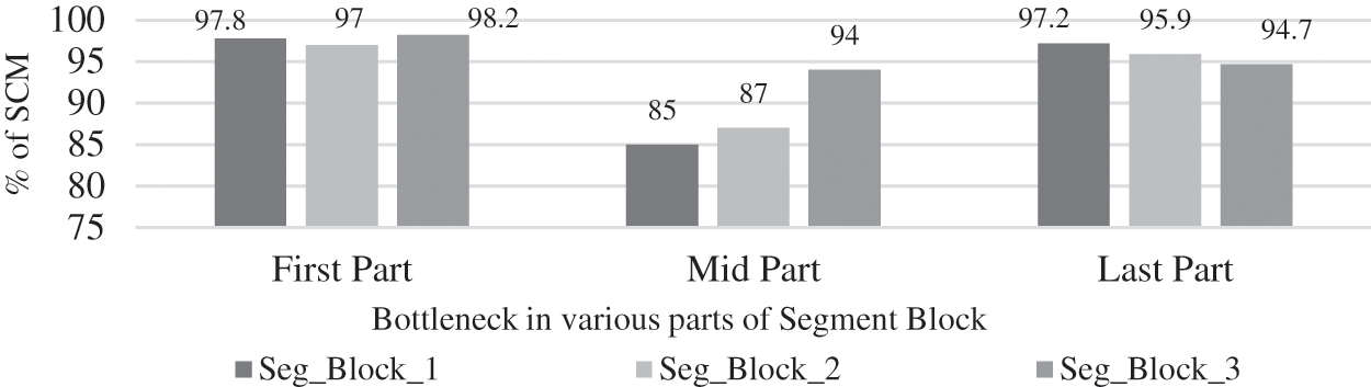
Figure 6: Ratio of SCM based on the impact of BS for single time steps in various block of segments
It can be summarized that (i) Except when the bottleneck occurs at the end of the ROS, the inevitable bottleneck situations increase the availability of the container migration destinations. (ii) On the VC trajectory, when the bottleneck occurs in the near future, the residual in-network time of VC participants is increased and the requirements for container migration are reduced. (iii) When migrating containers to the subsequent vehicles from the migrating source, the rate of effective container movement is high relative to vehicles travelling ahead of the migrating source. In Tab. 5 all the simulation outcomes are compared.
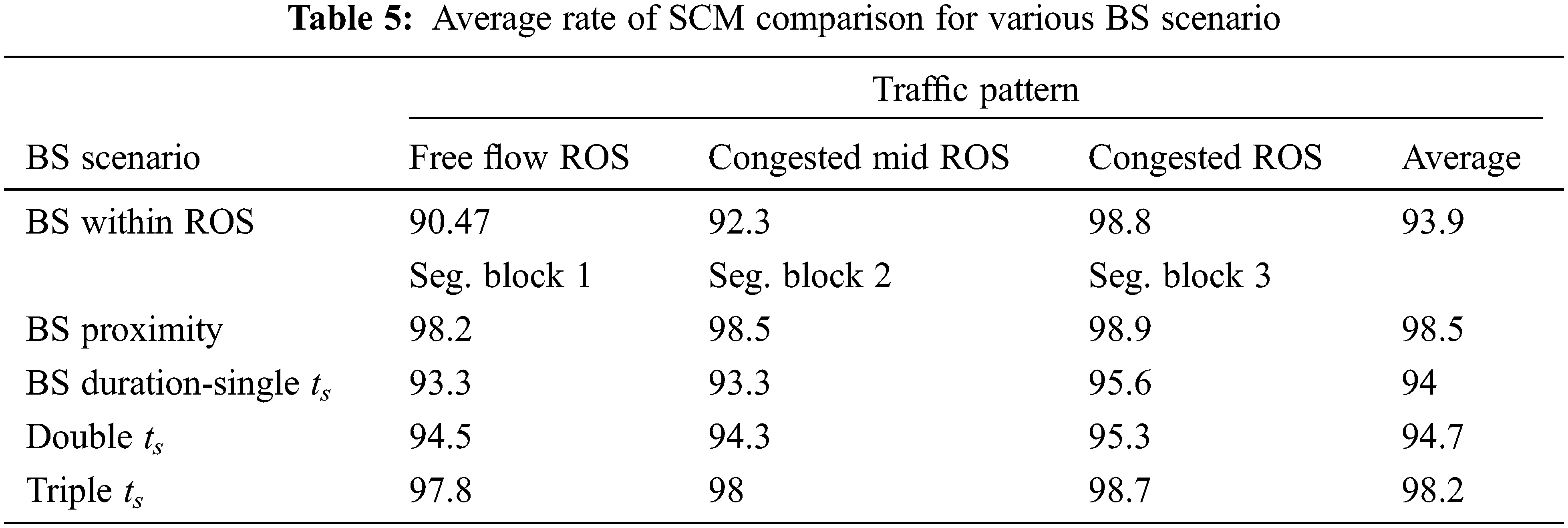
The MDWLAM [6] algorithm at high density of congestion with unrestricted resources results 97% of successful VM migrations, comparatively, this work results 98.5% of successful container migrations in the BS proximity scenario and 98.2% in the triple ts BS duration scenario.
This paper has proposed Nomadic Vehicular Cloud with two preeminent features: (i) only moving vehicles on the heavy traffic road are the NVC participants and (ii) Applying CTM as aid to decide about the initiation time of container migration. NVC is simulated with containers and 5G NR V2X PC5 interface. The usage of PC5 interface helps NVC to function independently without relying on the cellular network coverage. In terms of its portability and short start-up time, the lightweight containers are very apt for the functioning of NVC. From the simulations it is noted that with the estimation of the vehicle trajectory movement and the number of vehicles in a road with bottleneck situation, there is a significant increase in the rate of successful container migrations. In turn it also increases the success rate of NVC. For future work, the same proposal can be tested with more two-way lanes on the road, can apply additional 5G NR V2X features, such as mm Wave for NVC connectivity, can incorporate the effects of path loss models in NVC and can analyse the effect of dual mobility in NVC.
Funding Statement: The authors received no specific funding for this study.
Conflicts of Interest: The authors declare that they have no conflicts of interest to report regarding the present study.
1. P. Ghazizadeh, R. Florin, A. G. Zadeh and S. Olariu, “Reasoning about mean time to failure in vehicular clouds,” in IEEE Transactions on Intelligent Transportation Systems, vol. 17, no. 3, pp. 751–761, March 2016. [Google Scholar]
2. R. Florin, S. Abolghasemi, A. Ghazizadeh and S. Olariu. “Big data in the parking lot,” in Big Data Management and Processing, 1st edition, New York: Taylor and Francis, pp. 21.1–21.8, 2017. [Google Scholar]
3. L. Decker, “Supporting big data at the vehicular edge,” Ph.D. dissertation. Old Dominion University, Virginia, US, 2018. [Google Scholar]
4. A. Ghazizadeh, “Towards dynamic vehicular clouds,” Ph.D. dissertation. Old Dominion University, Virginia, US, 2020. [Google Scholar]
5. A. Ghazizadeh, P. Ghazizadeh and S. Olariu, “Job completion time in dynamic vehicular cloud under multiple access points,” in Int. Conf. on Cloud Computing, Cham, Springer, vol. 12403, 2020. [Google Scholar]
6. T. K. Refaat, B. Kantarci and H. T. Mouftah, “Virtual machine migration and management for vehicular clouds,” Vehicular Communications, vol. 11, no. 6, pp. 47–56, 2016. [Google Scholar]
7. A. Bazzi, G. Cecchini, M. Menarini, B. M. Masini and A. Zanella, “Survey and perspectives of vehicular Wi-Fi versus sidelink cellular-V2X in the 5G era,” Future Internet, vol. 11, no. 6, pp. 122, 2019. [Google Scholar]
8. H. Bagheri, M. Noor-A-Rahim, Z. Liu, H. Lee, D. Pesch et al., “5G NR-V2X: Toward connected and cooperative autonomous driving,” IEEE Communications Standards Magazine, vol. 5, no. 1, pp. 48–54, 2021. [Google Scholar]
9. R. Molina-Masegosa, J. Gozalvez and M. Sepulcre, “Configuration of the C-V2X mode 4 sidelink PC5 interface for vehicular communication,” in 14th Int. Conf. on Mobile Ad-Hoc and Sensor Networks (MSN), Shenyang, China, pp. 43–48, 2018. [Google Scholar]
10. M. Rondinone and A. Correa, “Definition of V2X message sets,” TransAID Consortium, 2018. [Google Scholar]
11. M. Tao, J. Li, J. Zhang, X. Hong and C. Qu, “Vehicular data cloud platform with 5G support: Architecture, services, and challenges,” in IEEE Int. Conf. on Computational Science and Engineering and IEEE Int. Conf. on Embedded and Ubiquitous Computing, Cham, pp. 32–37, 2017. [Google Scholar]
12. Z. Li, M. Kihl, Q. Lu and J. A. Andersson. “Performance overhead comparison between hypervisor and container based virtualization,” in IEEE 31st Int. Conf. on Advanced Information Networking and Applications, Taipei, Taiwan, IEEE, pp. 955–962, 2017. [Google Scholar]
13. C. F. Daganzo, “The cell transmission model: A dynamic representation of highway traffic consistent with the hydrodynamic theory,” Transportation Research Part B: Methodological, vol. 28, no. 4, pp. 269–287, 1994. [Google Scholar]
14. F. Sun, F. Hou and N. Cheng, “Cooperative task scheduling for computation offloading in vehicular cloud,” IEEE Transactions on Vehicular Technology, vol. 67, no. 11, pp. 11049–11061, 2018. [Google Scholar]
15. J. Shao and G. Wei, “Secure outsourced computation in connected vehicular cloud computing,” IEEE Network, vol. 32, no. 3, pp. 36–41, 2018. [Google Scholar]
16. R. Florin, A. Ghazizadeh, P. Ghazizadeh, S. Olariu and D. C. Marinescu, “Enhancing reliability and availability through redundancy in vehicular clouds,” IEEE Transactions on Cloud Computing, vol. 9, no. 3, pp. 1061–1074, 2021. [Google Scholar]
17. M. H. C. Garcia, A. Molina-Galan and M. Boban, “A tutorial on 5G NR V2X communications,”, IEEE Communications Surveys Tutorials, vol. 22, no. 3, pp. 1972–2026, 2021. [Google Scholar]
18. J. Lianghai, A. Weinand, B. Han and H. D. Schotten, “Multi-RATs support to improve V2X communication,” in 2018 IEEE Wireless Communications and Networking Conf. (WCNC), Barcelona, Spain, pp. 1–6, 2018. [Google Scholar]
19. K. Ganesan, J. Lohr, P. B. Mallick, A. Kunz and R. Kuchibhotla, “NR sidelink design overview for advanced V2X service,” in IEEE Internet of Things Magazine, vol. 3, no. 1, pp. 26–30, 2020. [Google Scholar]
20. A. Bazzi, B. M. Masini, A. Zanella and I. Thibault, “On the performance of IEEE 802.11p and LTE-V2V for the cooperative awareness of connected vehicles,” in IEEE Transactions on Vehicular Technology, vol. 66, no. 11, pp. 10419–10432, 2017. [Google Scholar]
21. R. Regin and T. Menakadevi. “Dynamic clustering mechanism to avoid congestion control in vehicular ad hoc networks based on node density.” Wireless Personal Communications, vol. 107, no. 4, pp. 1911–1931, 2019. [Google Scholar]
22. K. Ganesan, P. B. Mallick, J. Lohr, D. Karampatsis and A. Kunz, “5G V2X architecture and radio aspects,” in 2019 IEEE Conf. on Standards for Communications and Networking (CSCN), Granada, Spain, pp. 1–6, 2019. [Google Scholar]
23. S. Maheshwari, S. Choudhury, I. Seskar and D. Raychaudhuri, “Traffic-aware dynamic container migration for real-time support in mobile edge clouds,” in 2018 IEEE Int. Conf. on Advanced Networks and Telecommunications Systems (ANTS), Indore, India, pp. 1–6, 2018. [Google Scholar]
24. K. S. Gautam and T. Senthil Kumar, “Video analytics-based intelligent surveillance system for smart buildings,” in Springer Soft Computing, vol. 23, no. 8, pp. 2813–2837, 2019. [Google Scholar]
25. A. Vishnu Priya and A. k. srivastava, “Hybrid optimal energy management for clustering in wireless sensor network,” in Computers and Electrical Engineering, vol. 86, pp. 379–387, 2020. [Google Scholar]
 | This work is licensed under a Creative Commons Attribution 4.0 International License, which permits unrestricted use, distribution, and reproduction in any medium, provided the original work is properly cited. |