Computer Systems Science & Engineering DOI:10.32604/csse.2023.025189
Article

Vehicle Density Prediction in Low Quality Videos with Transformer Timeseries Prediction Model (TTPM)

D. Suvitha* and M. Vijayalakshmi

Department of Information Science and Technology, College of Engineering Guindy, Anna University, Chennai, 600025, Tamil Nadu, India
*Corresponding Author: D. Suvitha Email: suvitha19@gmail.com
Received: 15 November 2021; Accepted: 25 January 2022

Abstract: Recent advancement in low-cost cameras has facilitated surveillance in various developing towns in India. The video obtained from such surveillance are of low quality. Still counting vehicles from such videos are necessity to avoid traffic congestion and allows drivers to plan their routes more precisely. On the other hand, detecting vehicles from such low quality videos are highly challenging with vision based methodologies. In this research a meticulous attempt is made to access low-quality videos to describe traffic in Salem town in India, which is mostly an un-attempted entity by most available sources. In this work profound Detection Transformer (DETR) model is used for object (vehicle) detection. Here vehicles are anticipated in a rush-hour traffic video using a set of loss functions that carry out bipartite coordinating among estimated and information acquired on real attributes. Every frame in the traffic footage has its date and time which is detected and retrieved using Tesseract Optical Character Recognition. The date and time extricated and perceived from the input image are incorporated with the length of the recognized objects acquired from the DETR model. This furnishes the vehicles report with timestamp. Transformer Timeseries Prediction Model (TTPM) is proposed to predict the density of the vehicle for future prediction, here the regular NLP layers have been removed and the encoding temporal layer has been modified. The proposed TTPM error rate outperforms the existing models with RMSE of 4.313 and MAE of 3.812.

Keywords: Detection transformer; self-attention; tesseract optical character recognition; transformer timeseries prediction model; time encoding vector

1  Introduction

With the organization of moderate traffic sensor advancements, the detonating traffic information are carrying us to the age of big data. Hence transportation framework is evolved to use large information for effective metropolitan traffic controlling systems. Because of its broad use in numerous applications, object detection has become a more mature topic of study in recent years. Recently, video reconnaissance frameworks plays an essential aspect in controlling and processing the congestion in traffic areas. Since the most recent decade, vehicle detection and counting has turned out to be one of the trendiest propositions in various fields. Numerous scientists have concentrated on this field, and different methodologies have been proposed to detect vehicles from surveillance cameras. However, the video quality issue is a serious concern in terms of low cost surveillance equipment, which were not addressed in existing work. Not only in smart cities, internal areas like rural areas are also affected by traffic congestion which immediately impacts the accuracy of the vehicle counts. In this paper the above issues are addressed using three components, First component is DETR model is used as an immediate set forecast issue to cope up with the above problem. Encoder-Decoder component is used along with transformer for predicting the sequence. Self-attention technique is used to accurately train all discriminate relations among objects in order to eliminate replica predictions. Here, vehicles are predicted in a traffic video and is prepared with a group of loss function which performs bipartite matching among forecasted and data collected on real features. These components are evaluated for real time Indian traffic video dataset against Yolov5, Yolov3, Yolov2 and Yolo model as a baseline. DETR model has achieved precision rate of 0.948, recall rate of 0.931 and F1-score percentage of 93.9 which indicates DETR is the best detection model among other models. Second component is Tesseract Optical Character Recognition that has two parts, first part is text detection where the textual content inside the image is discovered. Second part is text recognition where the textual content is obtained from the image. As per the research work, date and time is recognized and extracted from the images of every frame in the traffic video. Then the length of the detected objects obtained from DETR model is computed for vehicle count. This vehicle count report along with date and time are added to the excel sheet. Third Component is the proposed work used for predicting the density of the vehicle for the future by using TTPM technique. The proposed model is evaluated against LSTM, LSTM in Self-Attention, BiLSTM in Self-Attention and Multihead-Attention model as a baseline. The proposed model error rate outperforms the existing models with RMSE of 4.313 and MAE of 3.812.

In outline, the significant contributions of this research are as per the following.

•   To adjust the transformer model with custom time series data, a few changes are made in the baseline model for the proposed work.

•   First, the NLP embedding layer of the model input is skipped, and the time series esteem is given as contribution to the model ltim∈Qn . Next the softmax classification function is discarded, and supplanted with regression cost function and here mean square error function is utilized.

•   To achieve the traffic density prediction accuracy, the time is encoded by joining a one-hot vector for every input. As a general rule, using this methodology for time coding, a trainable vector is consolidated with value, query, and key vectors, which permits the TTPM to choose the esteem of the vectors by itself rather than the cosine and sine technique.

•   The probability distribution are incorporated besides MSE function to boost the likelihood of data in the forecast interim.

The rest of this paper is structured in this fashion: Section 2 elaborates the related work on object detection and timeseries data prediction. The proposed framework is explained in Section 3. Section 4 deals with dataset description. Section 5 gives details about the experimental results and discussion of the proposed approach and Section 6 summarizes our work with future directions.

2  Related Works

2.1 Object Detection

Computer vision has enchanted an increasing number of interest in latest years. In the current ventures of computer vision, the evolution of deep learning and the associated algorithms of object detection and object counting have made notable progress in real world applications. Object detectors make use of deep learning models to extract features from input videos or images, classification, and localization respectively. Object detectors are classified into 2 types: Two-stage detector (Faster-RCNN) [1] and One-stage detector [2] and (SSD) [3]. Two-stage detectors have high-level localization and object detection veracity, while the one-stage detectors attain excessive inference speed. Two-stage detectors categorized with the aid of using Region of Interest and pooling layer. In Faster R-CNN, Region Proposal Network comes up with candidate object bounding boxes in the first stage. In the next stage, features are drawn out by the RoI Pooling technique from every candidate box for subsequent classification and bounding-box regression tasks [4]. While single-stage strategy make predictions based on anchors [5] or a grid of feasible object centers [6]. To get rid of the hand-designed additives like a non-max suppression technique and anchor technology that encodes the earlier information of the task a Transformer model is introduced. In practice Transformer has turned into an effective norm for NLP tasks, its function to computer vision stay confined. In computer vision, convolutional structures stay predominant. Motivated by NLP triumphs, numerous works take a stab at consolidating CNN-model with self-attention, some supplanting the convolutions completely and have not yet been scaled adequately on current hardware accelerator because of the utilization of specific attention techniques. Inspired by the Transformer scaling achievements in NLP, we explore different avenues by implementing a classic Transformer directly to the traffic videos for detecting objects (vehicles), with the least potential changes. Numerous estimations were attempted in the past to use Transformers in image processing. Self-attention mechanisms [7] were carried out in the local region for every pixel query rather than globally. Such multi-head self-attention wodge can take over convolutions entirely [8]. Sparse Transformers use tensile speculation to global self-attention model so it can be pertinent to images. To scale the attention model, the blocks of differing sizes can be used in the acute case at most beside the individual axes [9]. Most of the attention models exhibit positive effects on computer vision tasks, however, it needs complicated engineering to be carried out successfully on hardware accelerators. In this paper, we additionally integrate transformers with parallel decoding to get rid of the hand-designed additives like non-max suppression technique and anchor technology that encodes the earlier information of the task. The essential components of this groundwork, known as DETR, is an entity-based overall loss that outfits the exclusive predictions through bipartite matching, and an encoder-decoder transformer model. With a limited set of queried items, DETR motives the association link of the objects and the overall image heading on to output the entity of forecast in parallel.

2.2 Timeseries Data Prediction

Evaluating the future prediction derived from the past series of data is termed as timeseries forecasting. Three techniques used for time series prediction are Random models, Artificial Neural Network, and Support Vector Machine. ARIMA is the famous technique extensively used as a random model that is used as a base version in the maximum research area [10,11]. Here the data is in linear form and sticks to the normal distribution. Random models carry out exhaustively on linear data whereas actual-time series data is said to be nonlinear. The constraints in the random model in real-time data with unique functions like lacking values, multidimensional and nonlinear data’s are not much pertinent. Due to their ideal properties, neural networks are a greater appropriate technique than random models. Neural networks expertise to grasp a whole lot of linear and nonlinear information in the absence of professional knowledge and data speculation [12]. Different kinds of neural networks have established so far, a number of that have been utilized in predicting time series. For instance, ANN uses Multi-Layer Perceptron for anticipating the time-series data. Time Lagged Neural Network [13] is used for computing hidden features of time series that is used for foreseeing airline passengers time-series data. Some of the outstanding capabilities of MLPs that lead them to function well for time series computation are modelling nonlinearly, noise resistance, the pliability in the number of inputs and outputs that delivers the forecasting measure, and the improvement in multidimensional functionalities. Another type of NN is Convolutional Neural Network (CNN). CNN filters examine the periodic trends and predict the time-series data. 1-D CNN is commonly utilized for predicting time-series data. The determined values are stated as input to NN and multilayer-NN undetermined values are forecasted as output. WaveNet Convolution Neural Network is another time series prediction model where series features are uncorrelated to values. Here pooling layer isn’t used and so the scale of the input and the output of the NN are equal. This technique is too rapid due to the fact the recurrent network aren’t used and the size of the layers and kernels are increased. Long Short-Term Memory (LSTM) is another component of Recurrent Neural Network (RNN) is used for predicting time-series data [14,15]. Previous records are utilized by the usage of a recurrent network. The LSTM delivers a correct assessment by accessing the previous state input data and present state input data concurrently for anticipating the future data. Another form of LSTM used is Stacked-LSTM that makes use of a stack of LSTM to evaluate complicated patterns. Bidirectional [16] is the second version of LSTM and it uses both forward and backward layers for progression. Using a combination of CNN and LSTM in time-series prediction differs. CNN-LSTM is a combination of the spatial and temporal model. 1-D CNN accesses spatial data as input and accompanied by RNN with temporal data. Another technique of neural network community is the encoder and decoder model. An encoder encodes the input data positioned on a selected pattern after which a decoder decodes the output data relied on encoded data to provide the reliable output. This model has a greater perspective of the context to offer good performance. An extensive type of those sorts of networks is brought into time series prediction. i.e., LSTM sequence-to-sequence model with attention [17–19]. In this model, the effect of coded inputs on outputs is managed and implemented in turn of different expertise issues. Due to data nonlinearity in distinct time-series, challenges prevail to furnish in terms of long-term dependencies. To overcome the above issues TTPM is proposed for computing long-term sequences in order to enhance the overall performance the model.

Compared to the previous studies the attention on low-resolution object detection has been more fragile than that on high-resolution images. These images contain various objects with the background and they can possess adequate data about every object, which empowered deep learning models to extricate rich visual features from them and accomplish remarkable characterization execution. Nonetheless, there is no assurance that the profound deep learning models developed for high-resolution object detection will perform well for low-quality images, in which a large part of the object-related data is crumbled. Although prior research hasn’t taken this issue seriously, it should not be overlooked in real-time scenarios as detecting objects in a large high-resolution image causes low-resolution issues. To address this problem, DETR model is used for detecting object in low quality videos and this makes the structure simple compared to previous architectures that had handcrafted engineering, obstacles, thresholds, and hyper factors. In prediction phase, the most notable worry of the deep learning models are high time, memory intricacy and long term dependencies which thwarts model adaptability in numerous cases. To address this issue TTPM is proposed for computing long-term sequences in order to enhance the overall performance of the model and the time taken for computation is less compared to the existing models.

3  Proposed Framework

The Architecture contains 3 components namely, Detection Transformer, Tesseract Optical Character Recognition and proposed TTPM.

3.1 Detection Transformer

On a high level, this paper does object detection in custom-traffic images using CNN and then a Transformer to detect objects (vehicles) and it does so to attain bipartite matching training objective. This leaves the structure easy in comparison to the preceding architectures that have all styles of engineering, hurdles, thresholds, and hyper parameters. In Fig. 1. The image from the traffic video is given as an input image. Here we ought to detect all of the vehicles within the image and additionally where the vehicles are present along with what are the vehicle names. This is stated as object detection. The best classifier will detect the objects within the image along with the bounding boxes. These bounding boxes can overlap each other. There are several problems confronted here. First is to detect the objects and must inform how many objects are present wherein it no longer be same in each image. They may be more than one object of the same class and that they may be more than one object of various classes and additionally they’ve varied sizes and they may be overlapping throughout the whole image or they are able to occlude each other partially. The above problems confronted are very tough to address it. Previous works have carried out a variety of engineering on it with the aid of constructing detectors, pixel classification, and so on. They have used complex structures to solve the problem. But in this research work, simple architecture is used which goes from the high stage to the low stage implementation of each of the parts.

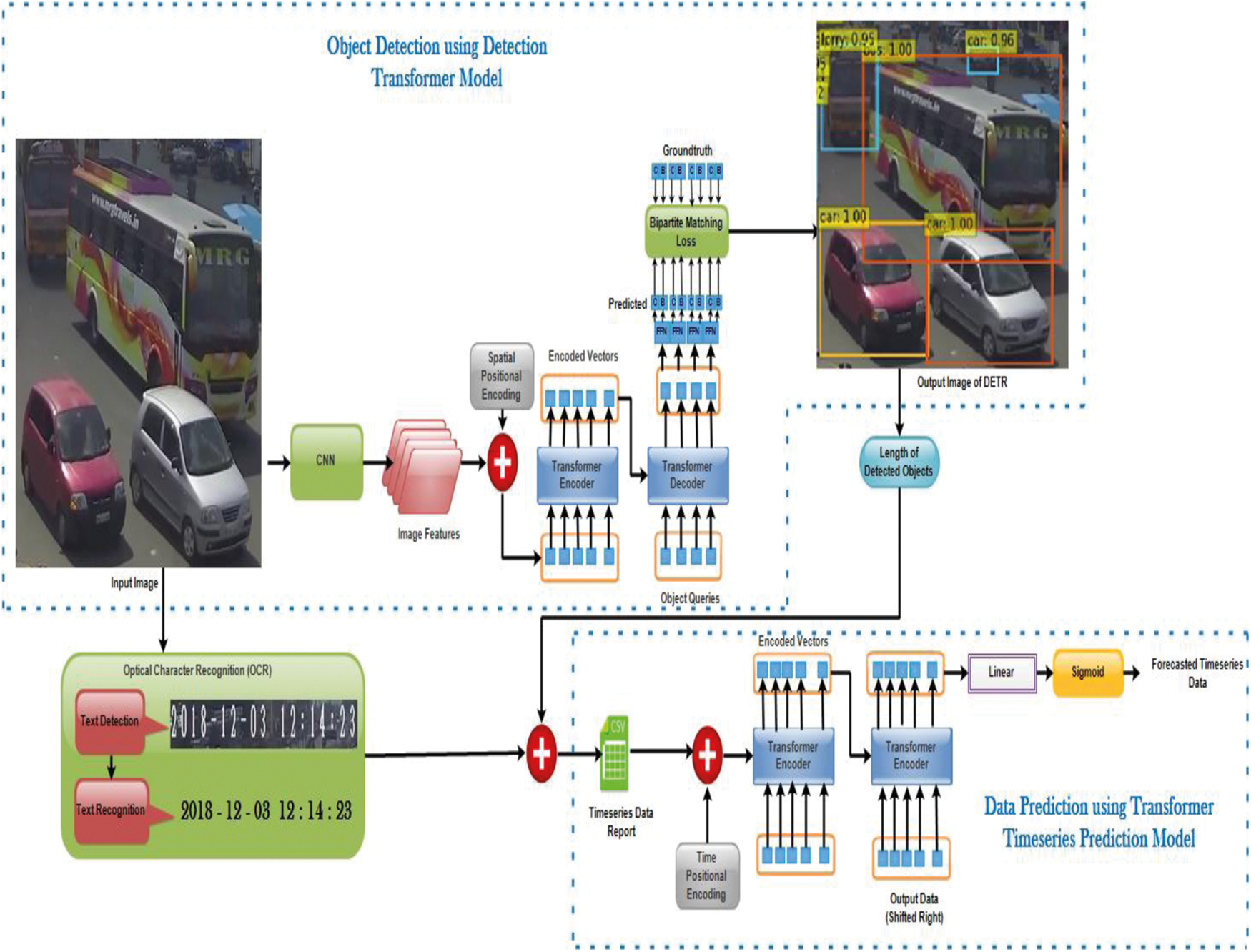
Figure 1: Architecture for the proposed work

In Fig. 1 the input image has 3 channels RGB is forwarded to the Convolutional Neural Network encoder. This CNN will scale it right all the way down to make higher channels. Still, that is an image forum and it is a higher-level illustration of the image with many greater feature channels however nevertheless has to discover the facts where those features are present in the image? This set of image features integrated with spatial positional encoding is sent to the transformer encoder-decoder component. These image features are flattened. The transformer encoder is certainly a sequence processing unit. It takes a collection of vectors as an input to the transformer encoder. Suppose if the image isn’t always a sequence, then image features have a bunch of channels with height and width. These features should be unrolled and flattened into one sequence collection. So mostly collection of C dimensional feature vectors are sent as input to the transformer encoder. This transformer encoder will remodel a sequence into similarly lengthy sequence features. The good thing about the transformer is in such a sequence, it has a multi-head self-attention layer and the encoder has instance vice or token vice Feed-Forward Neural Network. i.e., it is able to attend from every position to every position in a one-shot manner. So because it transforms the feature representation up the transformer layer at every step, it essentially aggregates information from anywhere within the sequence to everywhere else. In the image, the bounding box here is pretty huge so long-range dependencies occur. The transformer model structure actually makes sense here.

From the transformer encoder, it generates a similarly sized, equally shaped sequence. This data is taken and given as conditioning facts to the transformer decoder as a side input. The transformer decoder takes a series and outputs a series. The series it takes right here is known as object queries. It plays in a one-shot manner. It means it begins with the series collection of ‘N’ object queries and outputs the series collection with ‘N’ object queries.

Object queries used for inputting ‘N’ random vectors that provide essentially ‘N’ outputs to forecast ‘N’ bounding boxes. These object queries are fed into the Multi-head Attention model and one of these vectors from object queries gets transformed. As object queries ‘Q is transformed, it’s going to have the opportunity to essentially examine the features which is likewise a vector that comes from the transformer encoder, and that’s how the image data is gotten. Now this image feature integrated with object queries is sent to attention mechanism and outputs bounding box with a class label.

From Fig. 2 ‘N’ object queries are trained to ask ‘N’ different inquiries to the input images. In the first image, object queries ask what’s on the upper left part of the image that has small bounding box. Whereas in the next image, the object query queries what’s on the lowest right side part of the image? The solution to this is, in a higher layer, it is able to go back and asks the image more questions with the aid of sending ‘Q’ vectors of the attention mechanism and they’ll get back the ‘V’ vectors from the image features corresponds to the Q images.

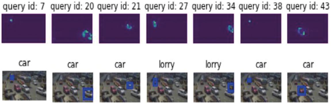
Figure 2: Object query mechanism

This Transformer encoder-decoder model outputs a set of box predictions. Each of the boxes has tuples that incorporate classes and bounding boxes (c, b). The class has vehicle class with bounding box (vehicle, x, y) and nothing class with bounding box ((Ø), x, y). Here nothing class (Ø) is a valid class. The set of images collected from the warehouse are manually annotated using LabelImg annotator with rectangular bounding boxes along with label. In this paper, I have converted LabelImg annotator to COCO annotator format to make the model to well understand. In manual annotation nothing class (Ø) is not annotated. So the question is how do you compare the two sets? i.e., with nothing class and without nothing class. The solution to this is bipartite matching loss.

N{(c,b)(∅,b)(c,b)(∅,ρ)(c,b)(∅,∗)(c,b)(c,b)(c,b)(c,b)}N↑↑Predicted_classifierGroundtruth_classifier (1)

In Eq. (1), the predicted classifier has the same amount of prediction i.e., ‘N’ is constantly fixed. Since it could forecast either a class or nothing class, it can predict anywhere from 0 to 5 objects. Whereas in the ground-truth classifier, it has only 2 instances in such case padding is done with nothing class. The ground-truth classifier ought to have size ‘N’. ‘N’ predicted classifier is compared with ‘N’ ground-truth classifier. To deal with this, correlate one predicted classifier with one ground-truth classifier and ordering need not be important. For instance, if there is one vehicle let’s say ‘lorry’ in this image is very prominent, the classifier should not encourage just because that the signal for that ‘lorry’ vehicle is stronger. So if the classifier has detected one object in an image, it should not detect the same object again in a slightly different place. This is said to be Bipartite Matching Loss. To compute the loss function, maximum matching should be computed. Loss function computation is shown in Eq. (2),

L((c,b),(c,b))=?→Howwellthese2agree?↑↑Predicted_object_on_left_imagePredicted_one_of_the_true_underlying_object_on_the_image (2)

•   If either of the class and bounding box is a nothing class, then there is no loss.

•   If the 2 classes agree and the 2 bounding boxes agree then it is good classifier it give negative loss or zero.

•   If the bounding boxes agree but the classes didn’t agree or if the classes agree but the bounding box didn’t agree or if the both didn’t agree then it is said to be bad classifier and becomes worst.

If the object on the left bounding box corresponds to the object on the right bounding box, then minimal matching need to be performed with the aid of using bipartite matching loss. So one to one understanding is made i.e., everything on the left bounding box is assigned precisely to one of the bounding boxes on the right such that the entire loss is minimized. The loss at the end of the matching is stated as training loss. So this solves the above issues, and it isn’t dependent on the order, because by reordering it, minimum matching will simplify and it will swap with it. i.e., if the ‘lorry’ vehicle is outputted multiple times, only one of these is going to be assigned to that class ‘lorry’, and the other ones can’t be assigned or forced to be assigned to a different one, and this one right here is going to incur a loss. So this solves the above troubles faced. There are different algorithms used for computing minimal matching. In this paper Hungarian algorithm is used for minimal matching loss which is given by the Eq. (3),

LHungarian(g,g^)=∑m=1N⁡[−log⁡f^σ^(m)(clm)+I{clm≠ϕ}Lbox(bom,bo^m)] (3)

where,

g - ground truth object

g^ - series of objects forecasted from m=1 to N

f^m - forecasted class

clm - ground truth class

bom∈[0, 1] 4 - defines vector of heightandwidth along with center x axis,y axis.

σ^=arg⁡minσ∈N⁡∑mN−Iclm≠ϕf^σ^(m)(clm)+I{clm≠ϕ}Lbox(bom,bo^m) (4)

In usage, we encumber the log-likelihood phase when clm = ϕ with the aid of using 10 aspects to interpret class variance. The comparable value among an object and nothing class ϕ do not rely on the forecast, this means the cost value is said to be persistent. The likelihood use here is f^σ^(m)(clm) rather than log probabilities. This model the forecasting class period in proportion to Lbox(bom,bo^m) in order to determine higher empirical conduct.

Several detectors are conflicted to detect bounding boxes in respect of few preliminary hypothecations, here we predict the bounding boxes straightly. Such techniques facilitate the performance difficulty with the associated scaling loss.

I – Identity operator assigns to 1, while clm ≠ ϕ else it assigns to 0. Bounding box loss is given by Eq. (5),

Lbox=λiouLiou(bom,bo^m)+λL1‖bom−bo^σ^(m)‖ (5)

The maximum utilized L1 loss contains unique scales for small and large bounding boxes despite the fact that their corresponding error is akin. To alleviate the difficulty caused a linear sequence of L1 loss and postulated IoU loss are used [20]. From Eq. (5), Liou(bom,bo^m) is said to be scale immutable. Here λiou and λL1 losses are scaled using the amount of sequence of detected objects.

3.2 Tesseract OCR

Text recognition in video frames and images is hard to detect due to tarnish videos, noise, low-resolution images, and so on. Optical Character Recognition (OCR) includes identification of text content on pictures and interpretation of those pictures to encode a text that the machine can handle it smoothly. People’s text and pictures are coherent to recognize the characters and pictures however PCs studies the text content from pictures as a progression of pixels. OCR is a conversion of scanned images (Smith 2007) into editable textual content for further handling. OCR is categorized into two components. The first component is textual content detection wherein the text content from the image is obtained. The second component used here is textual content recognition, the localization of textual content is essential for the textual content recognition whereas it derives the textual content from the image. Here the interaction may not be 100% exact and it may require some human mediation to address a few components that were not scanned accurately. To solve the above issues in this paper we delve into the concept of Tesseract OCR where tesseract library is a wrapper for google’s Tesseract OCR’s engine.

In Fig. 3 Structure of Tesseract OCR for recognizing Date and Time is shown. This paper presents Tesseract OCR for spotting date (day, month and year) and time (hours, minutes and seconds) from video frames. From the above Fig. 3 First the video with text is given as input and next the video is captured using OpenCV function Video Capture whereas it acquires a video file name to generate video in frame by frame manner. Next the frames are scanned and read. Before passing these frames to the Tesseract OCR, preprocessing is done. Two preprocessing techniques are used for this module. First technique is gray scale feature where the scanned images or scanned video frames need to be converted to grayscale image so that tesseract can provide better accuracy result. Second technique used here is binary thresholding which states that if the pixel value is above the threshold then the pixel is white whereas if the pixel value is below the threshold then the pixel is black. The binary threshold value set here is (200, 255). So in this way we have very concrete black and white image and because of that it is very easy for Tesseract OCR to predict or deliver the characters from image. After preprocessing, the combination of grayscale image feature and binary threshold image is sent to the Tesseract OCR to detect the textual content from the image. Here in these input frames date and time are detected from the image and then this localization of date and time content is crucial for text recognition component to extract the date and time content from the image. The above date and time extracted and recognized from the input image is integrated with the length of the detected objects obtained from DETR model. This gives the vehicle count report along with timestamp that are added to the excel sheet.

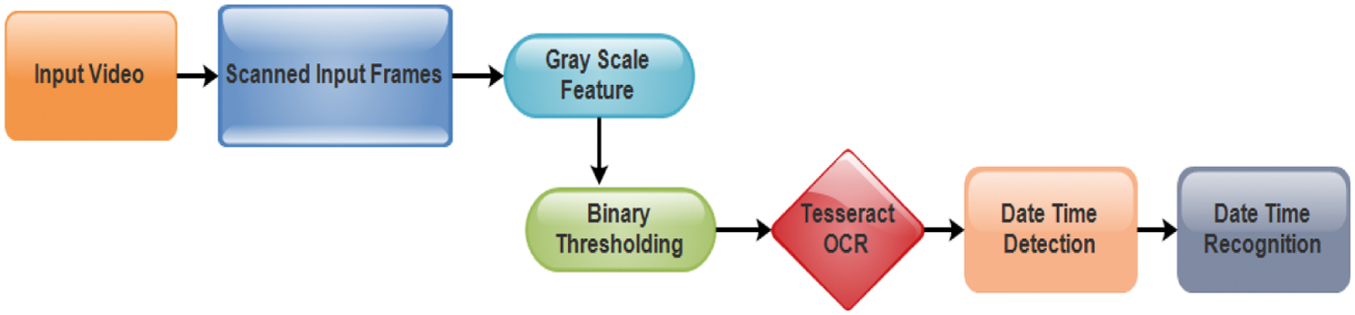
Figure 3: Tesseract optical character recognition for date time recognition

3.3 Proposed TTPM

To match the transformer with time-series data, a few alterations to the basic transformer model are given which is appeared in Fig. 1. First, the NLP-related embedding layer of the model input is skipped, and the time series value is provided as input to the model ltim∈Qn . Next the classification yield is omitted, and replaced with regression cost function and here mean square error function is used as the cost function. The transformer shows the Sin-Cosine strategy for time encoding, which essentially diminishes the precision of the model when predicting persistent time series. So, in this research work, the time is encoded by incorporating a one − hot vector for every input. In reality, utilizing this strategy for time coding, a trainable vector is incorporated with value, query, and key vectors, which allows the time-series transformer model to decide the esteem of the vectors by itself instead of cosine and sine strategy.

keyp=ipRkey (6)

valuep=ipRvalue (7)

queryp=ipRquery (8)

ip=ipc+posp (9)

queryp=(ipc+posp)Rquery=ipc×Rquery+posp×Rquery (10)

valuep=(ipc+posp)Rvalue=ipc×Rvalue+posp×Rvalue (11)

keyp=(ipc+posp)Rkey=ipc×Rkey+posp×Rkey (12)

ep,q=queryp×keyqTc (13)

ap,q=exp(ep,q)∑r=1n⁡exp(ep,r) (14)

lp=∑q=1n⁡ap,q×valueq (15)

where

ipc – embedding vector

posp- cosine-sine vector for pth time

The above equations are replaced with the following equation for proposed work

ip=concat(ipc,one−hot(p)) (16)

queryp=ipc×Rquery+apquery (17)

valuep=ipc×Rvalue+apvalue (18)

keyp=ipc×Rkey+apkey (19)

where

ipc - timeseries vector in Lt∈Qn

one−hot(p) – encoded vector in time p

apquery,apvalue,apkey – training vectors

The issue faced in the proposed strategy is the expansion of the input vector due to the increment in the size of the input time steps. Indeed the time encoding vector estimation gets to be greater than the input vector. To illuminate this issue, various time encoding vectors are utilized for diverse time interims. For instance in hourly information for one week, 24 vectors are utilized to indicate the hour and 7 vectors to specify the week days. These vectors are linked so time is encoded as 31 vectors. In expansion, date and time values are used rather than encoding the time completely from the starting of the series.

One of the exploration on transformer model, is supplanting Cosine and Sine area encoding with relative vector which greatly improves the performance. The provided solution of the revealed research is basically the same as encoding time by integrating a one − hot vector to the input data. In the corresponding elucidation, time is just coded in the value and key vector whereas the query vector relies upon the input which is free from time where no clarification has been given in the examination. The variation in computing the variable is shown in below equation. The rest of the computations are equivalent.

queryp=ipc×Rquery (20)

In this exploration, besides the MSE cost function, a different function is utilized dependent on a probabilistic methodology. Assume that ltim∈Qn is the value of series l in tim that is an n-dimensional vector. On the off chance p, is the pth measurement of the time series, the point is to demonstrate the conditional probability of the accompanying condition, P(Lp,tim0:T|Lp,1:tim0−1) represents the likelihood of forecasted value of the dimension p.

R0(Lp,tim0:T|Lp,1:tim0)=∏tim=tim0T⁡R0(Lp,tim|Lp,1:tim−1)=∏tim=tim0T⁡a(Lp,tim|θ(itim)) (21)

Among them, itim shows the decoder yield in time tim. Where a(Lp,tim|θ(itim)) shows the likelihood of event of the time series esteem value Lp,tim regarding the paired likelihood distribution parameters θ. Parameters used in distribution function is mean and standard deviation. Gaussian probability Eq. (22) is given below

agau(μ,σ)=(2πσ2)−1/2exp((l−μ)22σ2) (22)

μ(ip,tim)=RμTip,tim+fμ (23)

σ(ip,tim)=log⁡(1+exp(RσTip,tim+fσ)) (24)

The transformer model in Eqs. (23) and (24) are utilized to compute the probability distribution parameters based on the ultimate yield. Probability logarithms are attained to increase in Eq. (25) by using Eq. (21)

A=∑p=1N⁡∑tim=tim0T⁡log⁡(a(Lp,tim|θ(itim))) (25)

Cost function for the proposed work is given in Eq. (26)

A=∑p=1N⁡∑tim=tim0T−log⁡(2π)−log⁡(σp,tim)−((Lp,tim−μp,tim)22σp,tim2) (26)

The cost function is changed to the mean square error cost function by keeping the variance constant. During the training stage, the values are entered from the detection stage to the forecasting stage via the encoder-decoder attention layer, and this layer is trained in the decoder part by decreasing the function in Eq. (26) using the back-propagation algorithm. During the test period, the network cannot fit into the forecasted period. The network in this scenario uses the output whenever it needs which acts as an input afterward.

For better understanding the flowchart of the proposed methodology is shown in Fig. 4. The vehicle count dataset is first loaded and the first column indicates the vehicle count for every 10 min period, while the datetime column is in index position which is shown in Fig. 6. The Label Encoder class is used to replace the existing data in the first column of the data with the newly encoded data. Following that, feature scaling is used to perform preprocessing. The range of MinMaxScaler is used to normalise the features (0, 1). This standardized dataset is portrayed as a supervised learning issue. Given the veh_count at a previous time step, a supervised learning problem predicts traffic for the current hour (t). The next step is to create a data frame from the dataset, with each segment labelled suitably by variable number and time step. This allows a multivariate and univariate time series data to be used to plan a wide range of time step forecasting challenges. For supervised learning, the rows are separated into X and y segments when the data frame is returned, with t−1 representing X and t representing y. The next step is to split the dataset into training and test data. The input (X) is converted to a 3D position [batchsize, sequence_length, features]. The number of time steps is the sequence length, and each input timeseries is the feature. Next step is to build the TTPM model. Here classification RNN layers are supplanted with residual connections, layer normalization, and dropout. The subsequent layers are stacked several times. The transformer encoder blocks are stacked along with the multi-layer perceptron classification head. Aside from a heap of dense layers, transformer encoder’s tensor output should be curtail down to a vector of features for every data item in the present batch. A typical method for accomplishing this is to utilize a pooling layer. For this model, a GlobalAveragePooling1D layer is adequate. GlobalAveragePooling1D does average amongst all time-steps required for each feature dimension. If data format is `channels_last’, it emulates the input of the form (batch size, timesteps, features) and channels_first emulates to the input of the form (batch, features, timesteps). For the proposed work channels_last is used for the implementation with the temporal dimension of length 1. After building the model, train and evaluate the model using root mean squared error function and mean absolute error function. The proposed model is evaluated against LSTM, LSTM in Self-Attention, BiLSTM in Self-Attention and Multihead-Attention model as a baseline. The error rate of the proposed model outruns the existing models.

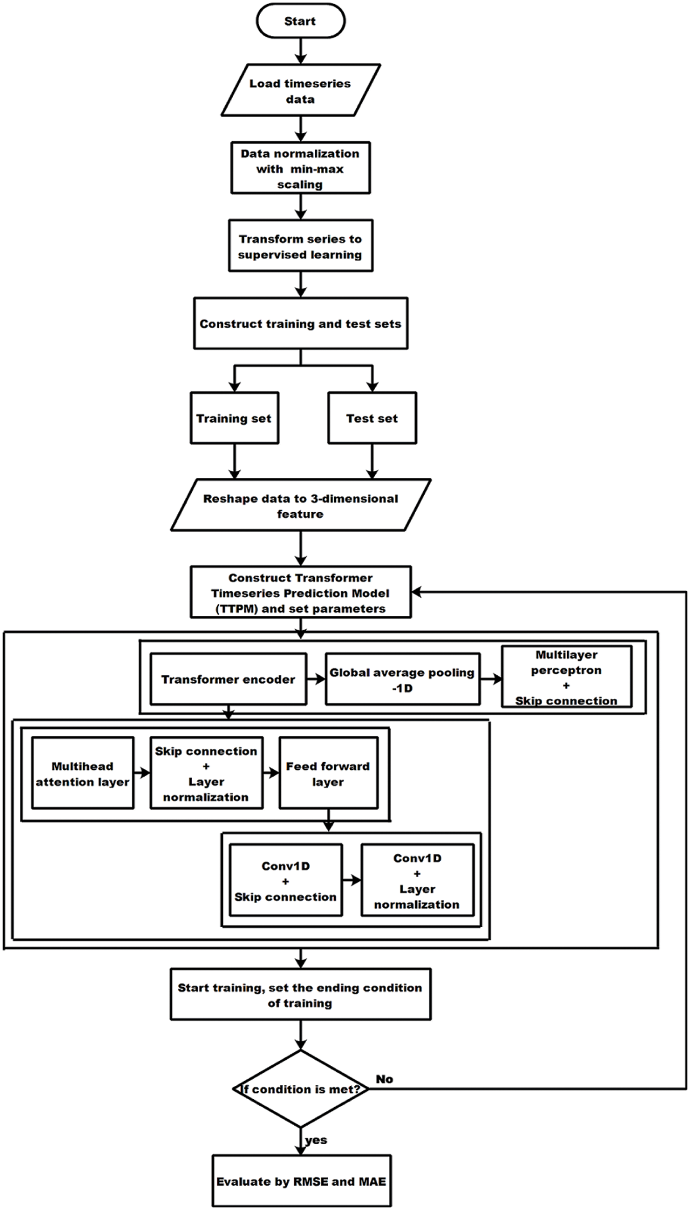
Figure 4: Flowchart of proposed methodology

Algorithm 1 explains the steps involved in the proposed TTPM

4  Dataset Description

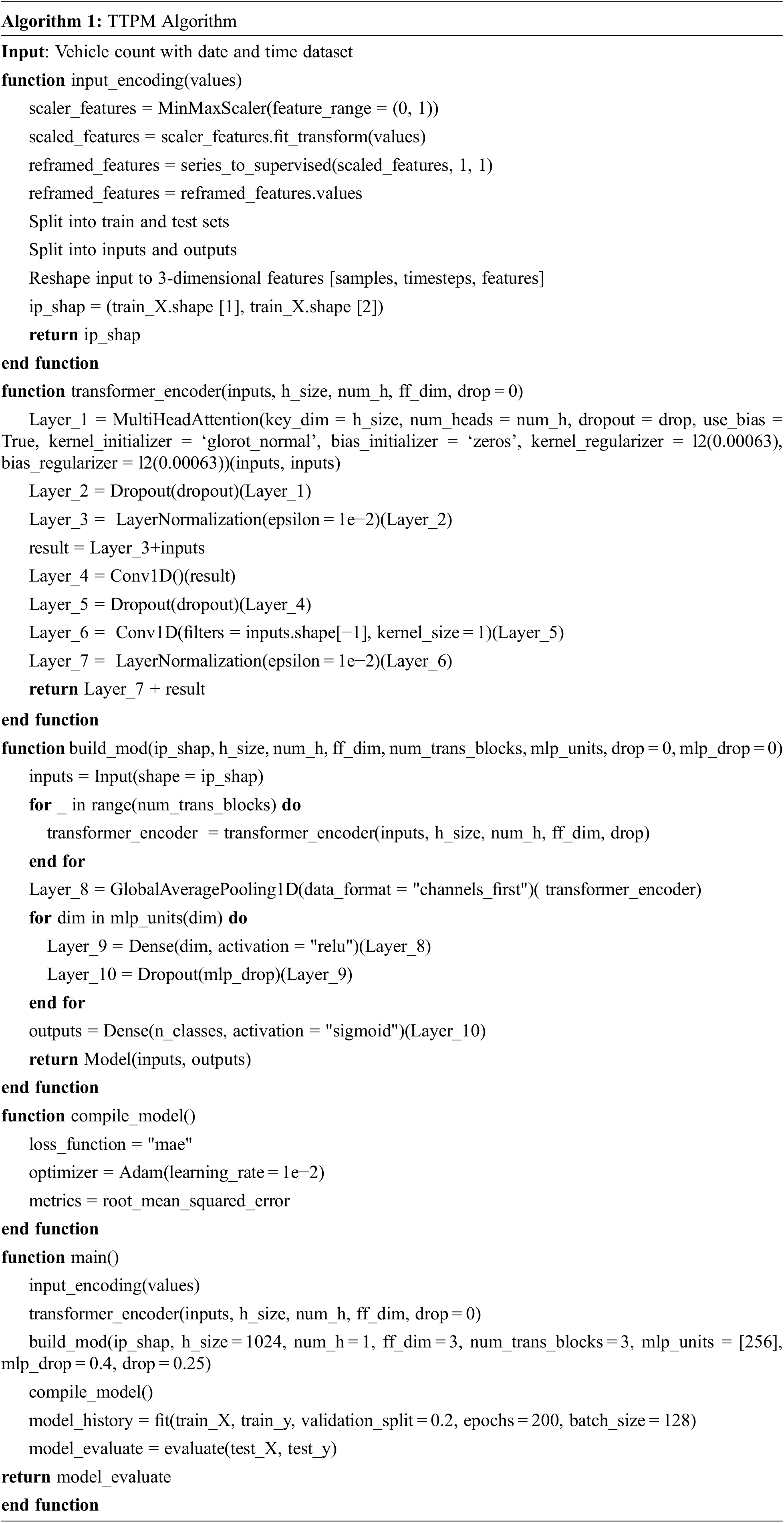
The traffic video is captured from seelanaicen patty surveillance camera from India at Salem city in the state of Tamil Nadu. Additional information about Salem city video data is accessible at the link https://drive.google.com/file/d/1HUa4Xgh05_5j8u6l1o0xo4llv0vvSv78/view?usp=sharing. In this link only 1 h video is uploaded. This video is collected for 21 days for every 24 h from the date of 01.12.2018 to 21.12.2018 which contains 357 gigabytes of data. But in this research work only day time videos are taken from morning 7:00 AM to evening 5:00 PM. In this paper day time video for 11 h is taken and for one day 99000 frames are generated, from that every 100th frame is taken for processing. Here LabelImg annotator is used for labelling the images along with rectangular bounding boxes to annotate objects on an image. For DETR model it accepts only COCO annotator single json file format. For this, LabelImg (Pascal VOC annotator) is converted to COCO annotator format i.e., by converting multiple json file to single json file which makes the DETR model to learn the data well. Annotations are done manually using 10 class objects i.e., Bike, Auto, Car, Lorry, Bus, Tempo, Van, Cycle, Jeep and Tractor. A wealthy annotations is made with orientated bounding boxes for ten classes additionally with one non empty class.

5  Experimental Results and Discussion

5.1 Analysis of Detection Transformer Model

DETR model is trained with a learning rate of 10−4 and the convolution backbone used in this model is resnet50 with a learning rate of 10−5. Before normalization layer, dropout of 0.1 is carried out for every multi-head attention and feed forward layer. With Xavier initialization, the weights are arbitrarily loaded. The number of encoding layers in the transformer used is 6, while the number of decoding layers is 6. The feed forward layers in the transformer blocks have an intermediate size of 2048, hidden layers have 256 dimensions, 8 attention heads are employed inside the transformer attentions, and the number of queries is set to 100. With λL1 = 5 and λiou = 2, a linear mixture of l1 and GIoU weight loss is assigned for bounding box regression. AdamW is the optimizer utilized here and 150 epochs are employed for training, with each epochs takes only 15 min to execute.

Fig. 5 shows how to see decoder attention for each predicted object. Forecasts are made with DETR model. Various colours are used for distinct objects using attention scores. Decoder focusses on the terminus of an object like vehicles shapes and sizes which is displayed in variant colours.

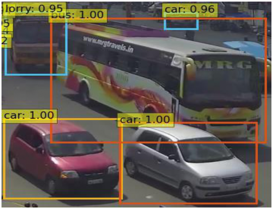
Figure 5: Vehicle detection using detection transformer

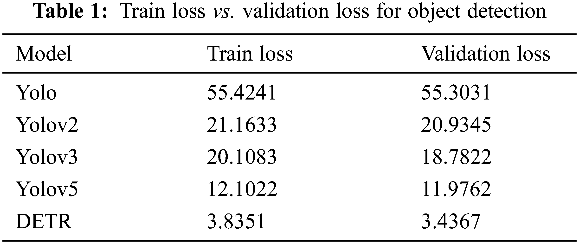
Tab. 1 represents the model comparison for object detection. From the below table it tells profound DETR model performs well with train loss 3.8351 and validation loss 3.4367 compared to the YOLO, YOLOv2, YOLOv3 and YOLOv5 models. These models take about more than an hour to run one epoch, whereas one epoch in the DETR model takes only 15 min. Even if numerous epochs are conducted, the time it takes to get the desired result is significantly shorter than with the existing model. Despite the availability of several existing model, the DETR model seem to be of greater efficiency and accuracy in data handling.

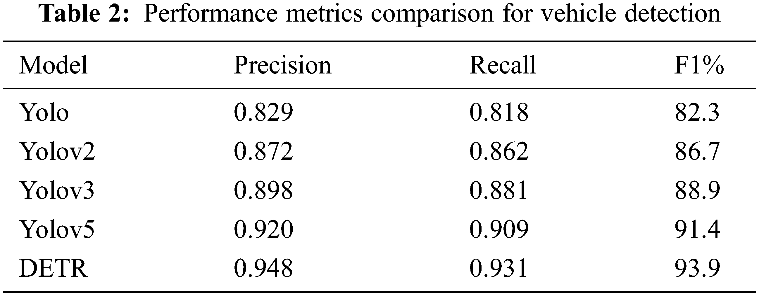
Precision, Recall and F1-score are utilized as assessment measures to verify the efficiency of the conducted tests on the trained YOLO, YOLOv2, YOLOv3, YOLOv5 and DETR models. The Computation technique is shown in Eqs. (27)–(29)

Precision=TPTP+FP (27)

Recall=TPTP+FN (28)

F1=2 ∗ Precision ∗ RecallPrecision+Recall (29)

True Positive(TP) - Accurate Detection

False Positive(FP) - Wrong Detection

False Negative(FN) - Missed Detection

The F1 score carried out as concession between Recall and Precision to evaluate the overall performance of the model as outlined in Eq. (29).

From Tab. 2 The Precision, Recall, and F1-scores of DETR detected vehicles were calculated and compared to the YOLO, YOLOv2, YOLOv3, and YOLOv5 models. Here DETR model precision rate is 0.948, recall rate is 0.931 and F1 score percentage is 93.9 which indicates the best detection model among other models.

5.2 Analysis of TTPM

Integration with DETR model and Tesseract OCR results in generating the vehicle count report as shown in Fig. 6. For data pre-processing, feature scaling (Min-Max scaler) is used for normalizing the features with range (0, 1). A dataset with length T-r+1 is created using the sliding window approach from time-series data with length T and window size r. The estimation problem will ultimately become an observer problem after normalization. The interaction is progressed using a sliding window that is partitioned into two stages: perception and revealed values, and predicting segment and unrevealed values. Two sections of the sliding window are employed in the training stage, and in validation stage the forecasting component is evaluated with the trained models and the real value of this part is utilized for working out metrics. This window pushes forward one step ahead and yields future data.

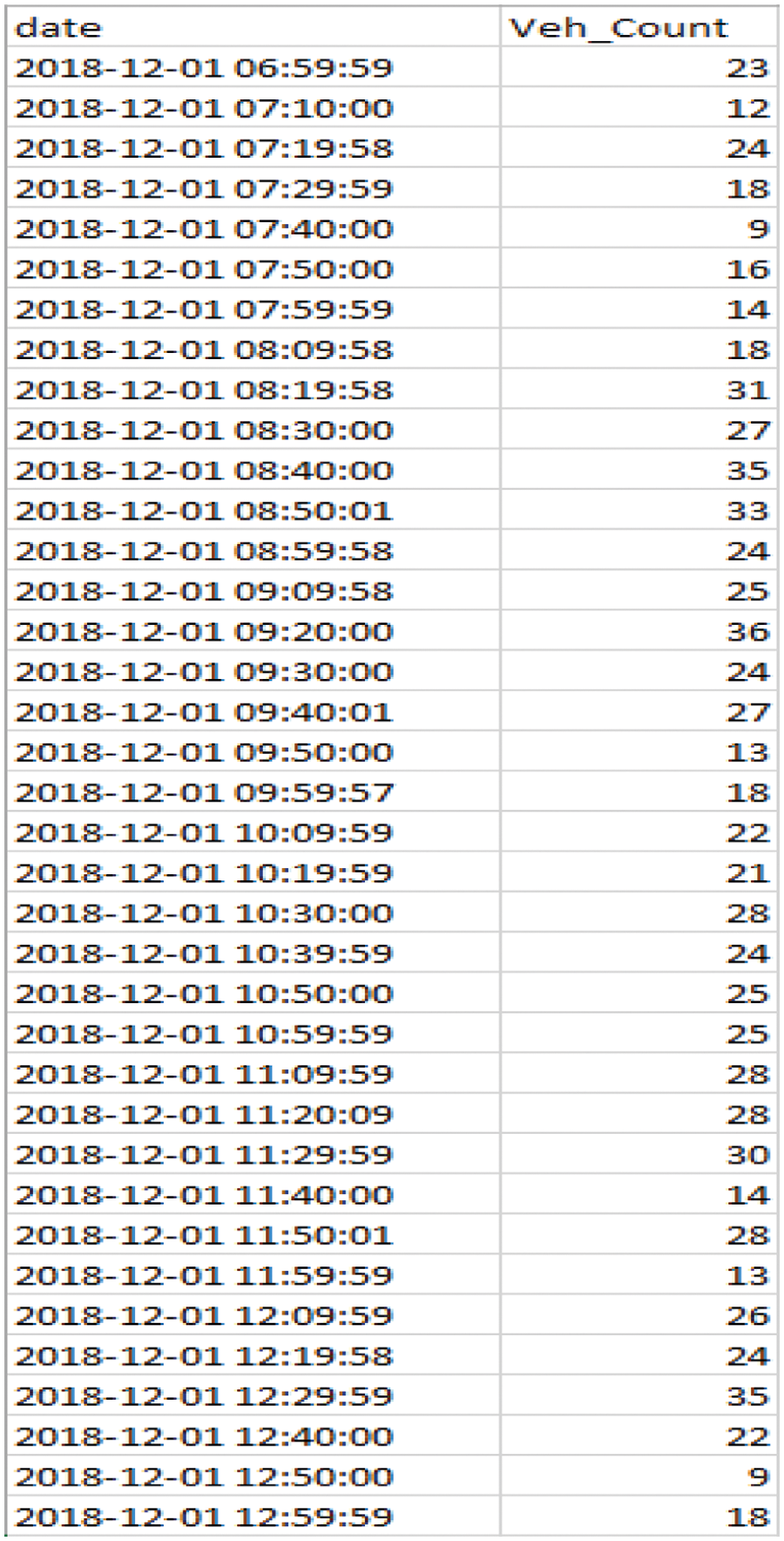
Figure 6: Vehicle count report

Summary of the proposed methodology is shown in Fig. 7. TTPM is trained with a learning rate of 10−4 for 200 epochs with batch size of 128 and validation split of 0.2. The number of transformer blocks used here is 3 with the Adam as optimizer. The transformer blocks have an intermediate head size of 1024 and 256 units of multilayer perceptron along with 1 attention heads employed inside the transformer attentions. Dropout of 0.25 is carried out for every multi-head attention and feed forward layer, and dropout of 0.4 is carried for multilayer perceptron layer. Proposed model incorporate residual connections, layer normalization, and dropout. The subsequent layer is stacked numerous times. The projection layers are carried out through keras.layers.Conv1D. The transformer encoder blocks are stacked with the addition of Multi-Layer Perceptron at the last head. Aside from a heap of dense layers, the output tensor has to be decreased down to a feature vector for every data point in the current clump. A typical method to accomplish this is to utilize a pooling layer using GlobalAveragePooling1D layer.

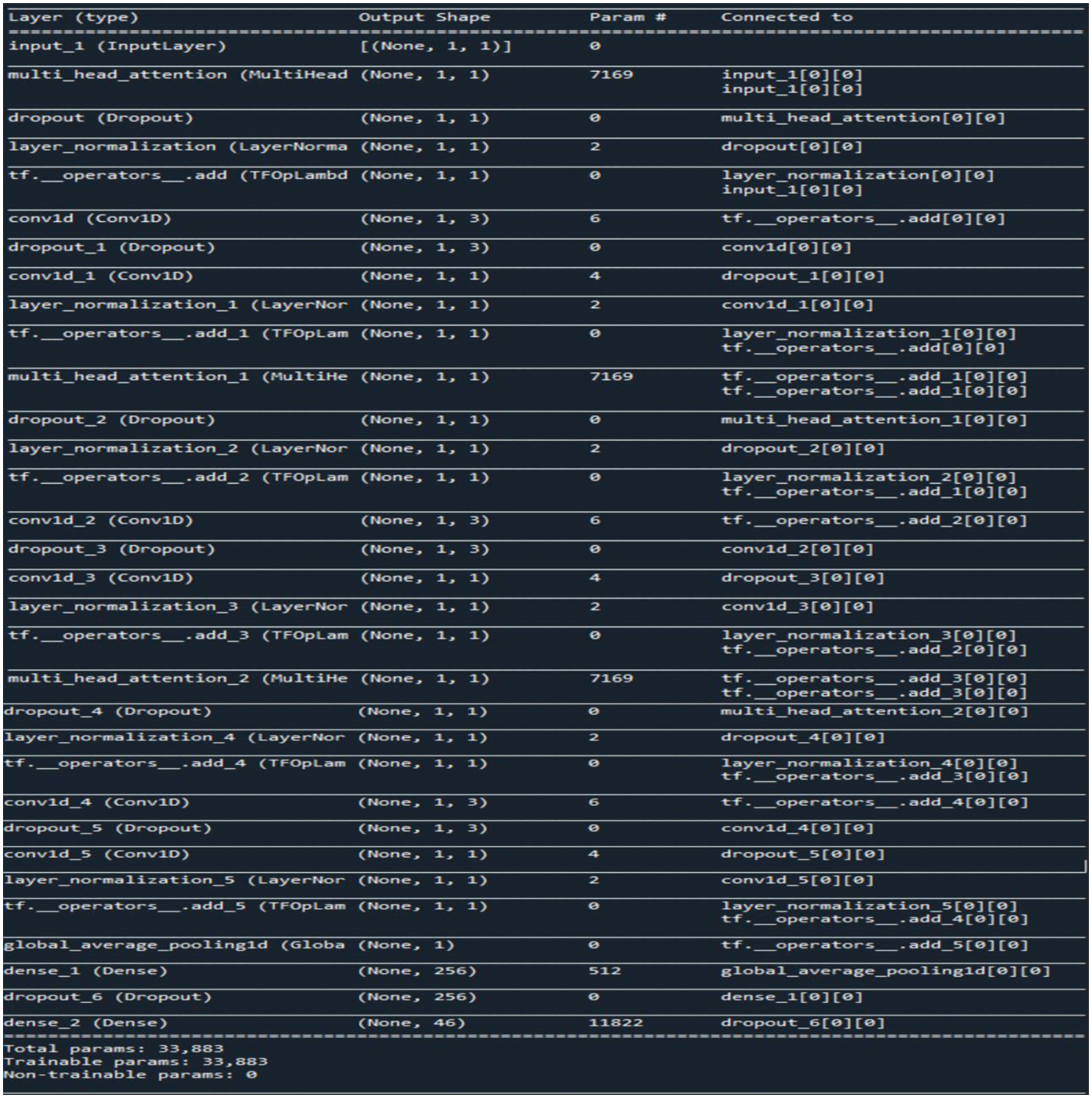
Figure 7: Summary of transformer timeseries prediction model

In Fig. 8 graph shows that the model is fitted for multi-step forecast. Here the model is trained for 200 epochs where the result of 200th epoch depends on 100 stages input. In this case long term data is learned from the training model. The blue lines specifies the ground truth data which is said to be the input and the red line shows the future predicted data and the dots specifies the values hidden from the model that is masked input.

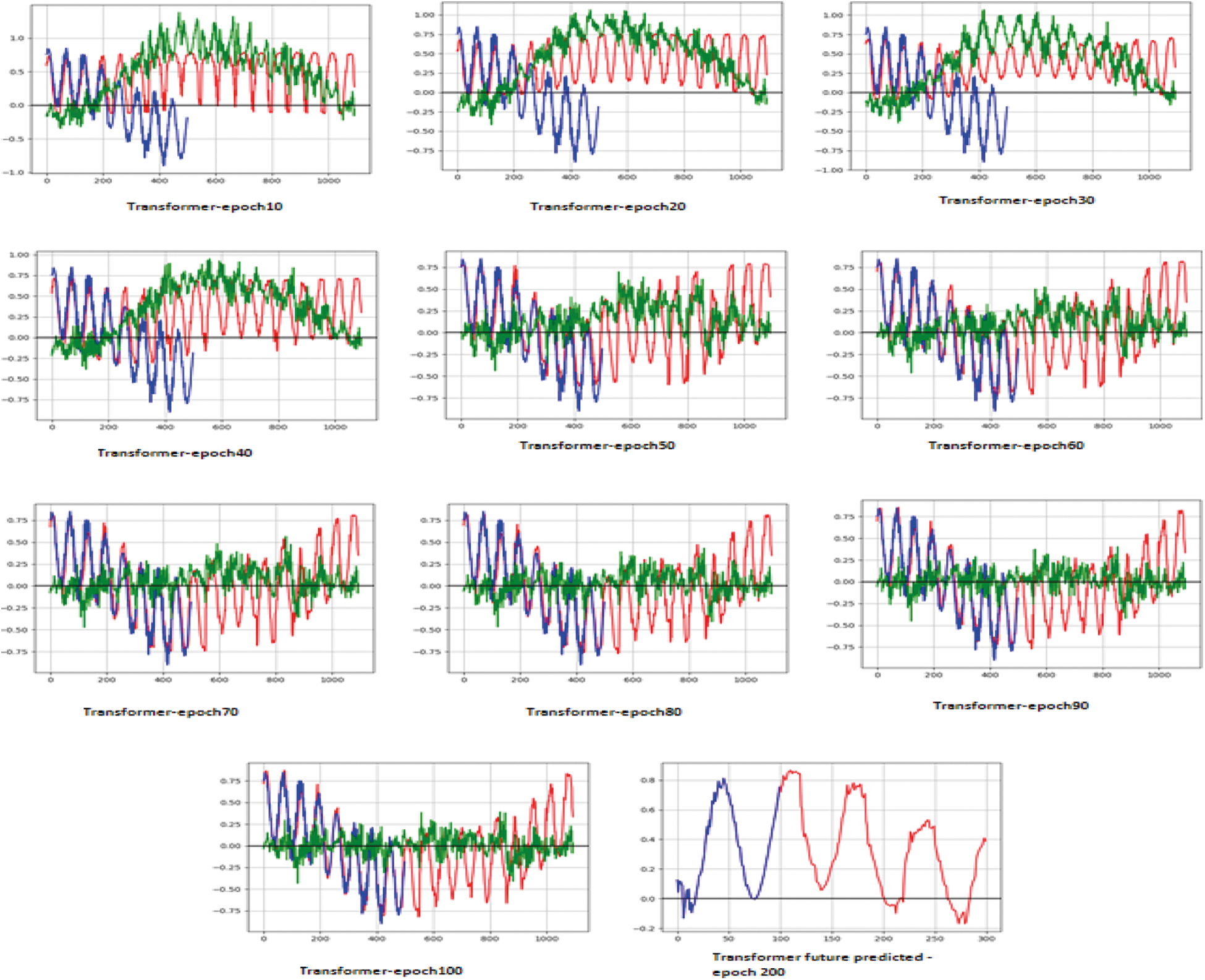
Figure 8: Multistep forecast for the proposed model

Fig. 9 illustrates on both the train and validation sets, the TTPM model performs well. This is deduced from the plot where the train and validation error settle around the similar point. Both the train and test errors are plotted at the end of the run. The complete data is forecasted after the model is fit. With these forecasted and actual data the model error rate is computed.

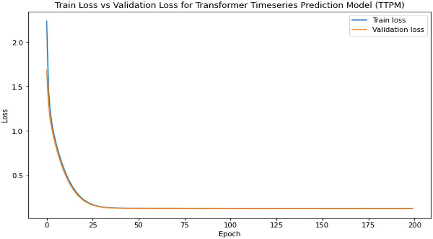
Figure 9: Train loss vs. validation loss for the proposed model

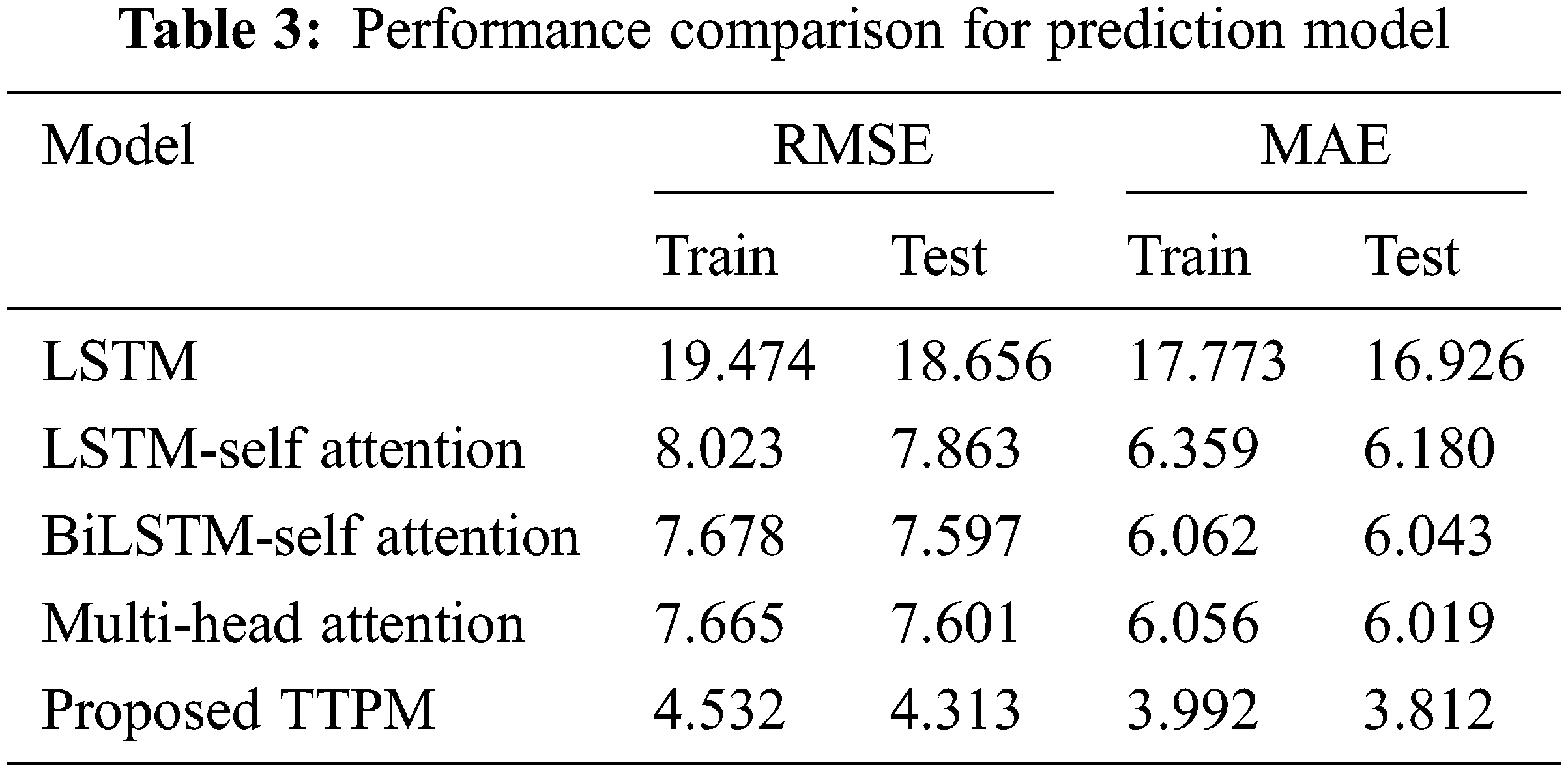
The Experimental tests were carried out using existing models with the RMSE and MAE objective function. All of the results were acquired from four unique experiments to validate the results and that results were compared to those of proposed technique. In Tab. 3. On both assessment metrics, the TTPM outperforms the other models with Train RMSE of 4.532 and Test RMSE of 4.313 and Train MAE of 3.992 and Test MAE of 3.812.

6  Conclusion

The proposed work uses low quality videos for counting and detecting objects which is highly challenging in vision based methodology. For object detection DETR model is used, here vehicles are predicted in traffic congestion area using a series of loss functions that perform bipartite coordination between estimated and real-world attributes. Compared to the existing models, DETR model has achieved precision rate of 0.948, recall rate of 0.931 and F1-score of 93.9 percentage. To recognize and extract the date and time of each frame in the traffic footage Tesseract OCR is used. The length of the recognized vehicles gained from DETR model is fused with output of Tesseract OCR to furnish vehicle report. TTPM model is proposed for predicting the traffic density of the vehicles for the future forecast. The error rate of the proposed model outperforms the existing models with RMSE of 4.313 and MAE of 3.812.

In the future research direction, detecting and counting the object for night scene data in Salem real-time traffic footage can be incorporated to anticipate future traffic density more precisely. And also the proposed work parameter count and precision can be improved by a hyper-parameter search with a refined learning rate, or an alternate streamlining optimizer.

Funding Statement: The authors received no specific funding for this study.

Conflicts of Interest: The authors declare that they have no conflicts of interest to report regarding the present study.

This work is licensed under a Creative Commons Attribution 4.0 International License, which permits unrestricted use, distribution, and reproduction in any medium, provided the original work is properly cited.