DOI:10.32604/csse.2023.025331
| Computer Systems Science & Engineering DOI:10.32604/csse.2023.025331 | |
| Article |
Conditional Generative Adversarial Network Approach for Autism Prediction
1Department of Computer Science and Engineering, Sri Eshwar College of Engineering, Coimbatore, 641202, Tamilnadu, India
2Department of Information Technology, Karpagam College of Engineering, Coimbatore, 641032, Tamilnadu, India
*Corresponding Author: K. Chola Raja. Email: kcholaraja21@outlook.com
Received: 20 November 2021; Accepted: 06 January 2022
Abstract: Autism Spectrum Disorder (ASD) requires a precise diagnosis in order to be managed and rehabilitated. Non-invasive neuroimaging methods are disease markers that can be used to help diagnose ASD. The majority of available techniques in the literature use functional magnetic resonance imaging (fMRI) to detect ASD with a small dataset, resulting in high accuracy but low generality. Traditional supervised machine learning classification algorithms such as support vector machines function well with unstructured and semi structured data such as text, images, and videos, but their performance and robustness are restricted by the size of the accompanying training data. Deep learning on the other hand creates an artificial neural network that can learn and make intelligent judgments on its own by layering algorithms. It takes use of plentiful low-cost computing and many approaches are focused with very big datasets that are concerned with creating far larger and more sophisticated neural networks. Generative modelling, also known as Generative Adversarial Networks (GANs), is an unsupervised deep learning task that entails automatically discovering and learning regularities or patterns in input data in order for the model to generate or output new examples that could have been drawn from the original dataset. GANs are an exciting and rapidly changing field that delivers on the promise of generative models in terms of their ability to generate realistic examples across a range of problem domains, most notably in image-to-image translation tasks and hasn't been explored much for Autism spectrum disorder prediction in the past. In this paper, we present a novel conditional generative adversarial network, or cGAN for short, which is a form of GAN that uses a generator model to conditionally generate images. In terms of prediction and accuracy, they outperform the standard GAN. The proposed model is 74% more accurate than the traditional methods and takes only around 10 min for training even with a huge dataset.
Keywords: Autism; classification; attributes; imaging; adversarial; fMRI; functional graph; neural networks
Autism, often known as autism spectrum disorder, is a group of disorders marked by difficulties with social skills, repetitive activities, speech, and nonverbal communication. Autism is a spectrum disorder, which means that each individual with autism has their own mix of strengths and problems [1]. People with autism can learn, reason, and solve problems in a variety of ways, ranging from highly proficient to severely handicapped. Rare persons with ASD may require a great deal of assistance in their everyday lives, while others may require less assistance and, in some circumstances, live completely independently. Autism can be caused by a variety of reasons, and it is frequently accompanied by sensory sensitivity, physical difficulties such as gastrointestinal (GI) diseases, seizures, or sleep abnormalities, as well as mental health issues such as anxiety, depression, and concentration problems.
Autism symptoms generally develop between the ages of two and three. Some developmental impairments can show up much sooner, and it's not uncommon to be identified as early as 18 months [2]. People with autism who receive early intervention have better results later in life, according to research. One out of every 160 children in the globe is thought to have an ASD. This number is an average, and the prevalence recorded in different research varies a lot. Because of the high incidence rate and diverse character of ASD, several researchers have turned to machine learning for data analysis rather than traditional statistical approaches. This is the motivation behind us, also to study this topic and come up with a better solution for more accurate ASD prediction.
Machine learning refers to any type of computer software that can learn on its own without the assistance of a programmer [3]. Machine learning is a sub branch of artificial intelligence, while deep learning is a sub branch of machine learning. Deep learning is a set of algorithms that simulates the thinking process by processing massive amounts of data. In terms of complex abstractions, deep learning models are nimble and result oriented. Although deep belief networks, generative models, propositional formulae, and Boltzmann machines are included in the list, they are primarily based on Artificial Neural Network.
Recent advancements in neuroscience and brain imaging have opened the way for a better understanding of the brain's function and structure [4]. For evaluating brain pictures, traditional statistical methods focused on mass-univariate approaches. However, these approaches ignore the interdependence of multiple areas, which is increasingly recognized as a valuable source of information for the diagnosis of numerous brain disorders.
Machine learning models as shown in Fig. 1 above, on the other hand, typically use the connection between different brain areas as its feature vectors and are hence favoured over other approaches. The use of machine learning approaches to neuro imaging data in these groups is expected to lead to a better understanding of patterns of neurobiological functioning that would otherwise go undetected by conventional methods. These advancements will help us not only detect these illnesses, but also better understand the processes that contribute to their genesis. Deep learning is a subset of machine learning that is essentially a three-layer neural network. These neural networks try to mimic the human brain's function by letting it to “learn” from vast quantities of data [5]. While a single-layer neural network may generate approximate predictions, more hidden layers can assist to optimize and improve for accuracy. Deep learning eliminates some of the data pre-processing that machine learning normally entails. The majority of ASD and normal control diagnoses are based on prior distinctive characteristics derived from brain imaging [6]. The hidden characteristics of ASD, which may be utilized to accurately differentiate between ASD and normal controls, are difficult to detect and identify solely by reading brain images, due to the complexity and limited information about the pathogenic process of ASD. Traditional machine learning approaches use a variety of feature extraction and classification techniques, but with deep learning, feature extraction and classification are done intelligently and holistically [7].
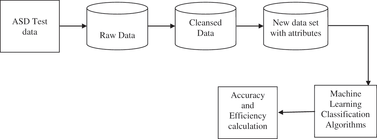
Figure 1: A typical classification pipeline using machine learning methods
Deep learning algorithms which are considered as the subset of artificial intelligence helps to build a mathematical model based on the samples or features extracted during training phase and further help in prediction or classification of new test vector based on the learning that has happened [8,9]. In our proposed work, the generator will make use of the features or statistics to generate results based on the brain image while the discriminator will try to filter the results and feedback the output to generator again to do the process in a loop until a satisfactory condition is reached. This along with the proper choice of loss function helps to make the system more efficient and can also be seen as an alternative to relevance feedback mechanism but without the end user intervention in the process.
The paper is arranged with 5 sections. Literature survey is described in second section. Proposed work is discussed in third section. Experiment and result is discussed fourth section. Conclusion is stated in fifth section.
Autism is a neuro developmental condition marked by social interaction and communication problems, as well as limited and repetitive behaviour. During the first three years of a child's life, signs are visible and typically emerge gradually. After completing developmental milestones at a normal rate, some autistic children experience regression in their speech and social abilities.
Researchers are employing machine-learning approaches to enhance diagnosis, categorize the disease into subgroups, and give support to those on the autism spectrum [10]. Machine learning may also aid researchers in better understanding why the nature and severity of autism symptoms differ from person to person. Machine learning is used to evaluate brain scans and clinical data, such as beginning age and drug use.
Jamal and colleagues used functional brain connectivity measurements generated from children's electro-encephalograms (EEG) during face perception tasks to examine the existence of autism [11]. For the extraction of brain connection characteristics, the least and maximum occurring synchro states for each subject are chosen, which are then utilized to classify these two groups of participants. For the classification problem, we investigated discriminant analysis and support vector machine, both using polynomial kernels, among many supervised learning approaches.
Azamimi Abdullah et al. created an experiment on utilizing Autism Spectrum Questions (AQ) to generate models with a greater capacity to identify ASD [12]. The feature selection methods used in this study were Chi-square and Least Absolute Shrinkage and Selection Operator (LASSO) to select the most important features for three supervised machine learning algorithms: Random Forest, Logistic Regression, and K-Nearest Neighbors with K-fold cross validation. The findings showed that Logistic Regression had the best accuracy, scoring 97.541 percent using a model with 13 characteristics chosen using the Chi-square selection approach.
For any machine learning model to perform better, sufficient supervised information is essential. Kong et al. have discussed about using active generative adversarial networks for the purpose of image classification [13].
Rezaei et al. have proposed a novel adversarial network that helps to learn multiple tasks at the same time [14]. A weighted loss method is discussed that takes care of mitigating imbalance data problem frequently encountered in the field of medical imaging.
Xiaan et al. classified ASD patients and normal controls using several SVMs [15]. The Autism Brain Imaging Data Exchange (ABIDE) database was used to acquire resting-state functional magnetic resonance imaging (fMRI) data of 46 TC and 61 ASD patients for testing. This will be extremely beneficial to physicians, since it will allow them to diagnose Autism Spectrum Disorder at an earlier stage [16]. Using four highlights and a second request polynomial bit in SVM, complex arrange parameters were used to design and assess discriminating examination, as well as a bolster vector group of classifiers with a maximum exactness of 94.7% is achieved with the proposed method.
Speech recognition, image classification, automotive software engineering, and neuroscience have all benefited from convolutional neural networks (CNN). A combination of algorithmic innovations, improved processing resources, and access to a vast quantity of data has enabled this remarkable achievement. Sherkatghanad et al. focused on using a brain imaging dataset to automate the identification of ASD [17]. They identified ASD patients using the most frequent resting-state fMRI data from the Autism Brain Imaging Exchange, a multi-site dataset (ABIDE). Based on functional connectivity patterns, the suggested method was able to identify ASD and control patients.
Heinsfeld and others looked analysed brain imaging data from ASD patients from a global multi-site database called ABIDE (Autism Brain Imaging Data Exchange). Their study's objective was to use deep learning algorithms to identify autism spectrum disorder individuals from a large brain imaging dataset purely based on their brain activity patterns [18,19]. By reaching 70% accuracy in identifying ASD vs. control patients in the dataset, the researchers enhanced the state-of-the-art. The categorization patterns reveal an anticorrelation of brain activity between anterior and posterior regions of the brain, which supports existing empirical findings of anterior-posterior disturbance in brain connection in autism spectrum disorder.
Autism spectrum disease is a neurological and developmental condition, according to Yin et al. [20]. The traditional method of diagnosing ASD involves observing behaviors and interviewing the patient. Finally, they train a deep neural network with enhanced features, which achieves 76.2 percent classification accuracy and a 79.7% receiving operating characteristic curve (AUC). They attained a classification accuracy of 79.2 percent and an AUC of 82.4 percent when they combined the DNN with the pre-trained AE and trained it using raw data.
3 fMRI Data and the Deep Learning Approach
Deep neural networks are made up of several layers of linked nodes, each of which improve and refine the prediction or categorization. Forward propagation refers to the flow of calculations via the network. The visible layers of a deep neural network are the input and output layers. The deep learning model ingests the data for processing in the input layer, and the final prediction or classification is generated in the output layer.
The brain activity is measured by functional magnetic resonance imaging (fMRI), which detects variations in blood flow. The fact that cerebral blood flow and neuronal activity are linked is used in this method. When a part of the brain is used, blood flow to that part of the brain increases as well. Functional Magnetic Resonance Imaging is one of the most widely utilized imaging modalities for studying human brain processes and diagnosing and treating brain diseases.
Artificial intelligence advancements and the advent of deep learning techniques have showed promise in improving the interpretation of fMRI data. Deep learning approaches have quickly become the gold standard for processing fMRI data sets, resulting in improved performance in a variety of fMRI applications. Deep learning is an end-to-end learning method that can minimize domain knowledge requirements by alleviating feature engineering requirements. fMRI data can be viewed as pictures, time series, or image series in the context of deep learning. As a result, various DL models, such as convolutional neural networks and recurrent neural networks, may be created to analyse fMRI data for various tasks.
The term “brain parcellation” refers to the process of establishing discrete partitions in the brain, whether those partitions are areas or networks made up of numerous discontinuous but closely interacting regions. Most fMRI investigations begin by identifying regions of interest (ROI) and then computing an average BOLD time series. Some research have indicated that taking the average isn't always the best option, and indorse using principal component analysis (PCA) to extract the main eigen-time series from the ROI(s).
In a resting state, when processing external inputs, the phrase “functional connectivity” refers to correlations in activity among geographically different brain areas. Several functional neuro imaging techniques, notably PET and fMRI, have been used to assess functional connectivity. Based on the premise that the time-series is stationary, whole time-series methods seek to analyse the relationships contained within the whole time-series of fMRI images.
4 Generative Adversarial Network for ASD Prediction
A generative adversarial network (GAN) is a type of machine learning framework in which two neural networks compete in a game against each other. The two networks in the GAN architecture will compete to generate new data based on the training set statistics, which will produce better results than the originals. With the help of labels, GAN modelling can be improved, which can assist with the discrimination process. Conditional generative adversarial networks, or C-GANs, are used to accomplish this. We use C-GANs because conventional GANs do not allow us to control the sample types that are generated. C-GANs use certain conditions to produce the output samples. Different class labels can be encoded and integrated into discriminator and generator models in a variety of ways. The discriminator is then fed the newly generated sample set to see if the output is true or false, and the sample is chosen accordingly. Fig. 2 depicts the proposed procedure for having multiple conditions.
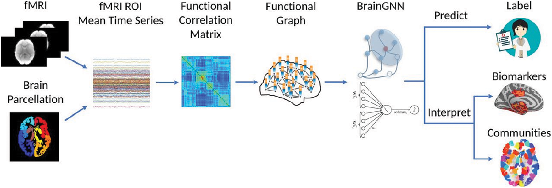
Figure 2: Interpretable brain graph neural network for fMRI analysis
When the objects appear to be identical and practical, the generator receives positive feedback. When the merged object is empty, the feedback will be negative, indicating that the objects are different is shown in Fig. 3. In comparison to traditional generative adversarial network models, we can generate and classify a larger number of samples this way.
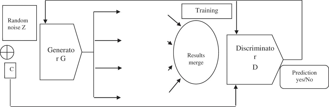
Figure 3: Generative adversarial network based deep learning
Deriving features from data is a crucial step in creating a solution using ML models. Although much effort is being done to better understand the neurobiological foundations of ADHD and ASD, identifying the specific neurobiological correlations remains a difficulty, causing problems with feature selection. The time series of voxels or regions of interest is used to derive fMRI-based characteristics. ROIs can be established using clustering techniques and structural qualities such as anatomical atlases or functional aspects of fMRI time series. These techniques can also be used on components created with the Independent Component Analysis (ICA) approach. Without explicit previous information, ICA is a data analysis approach that discovers the most maximally independent components of the brain.
The behaviour of functional connectivity between brain areas has been demonstrated to be dynamic rather than static. As a result, the strength of the link between the two regions may shift over time. Dynamic Functional Connectivity (DFC) is a notion that is becoming increasingly essential in understanding cognitive processes.
This dynamic behaviour is often discovered using a sliding window framework, in which a window of size w is slid across the time series and functional connectivity between all areas is calculated based on the time points covered by the window. The window moves over s items and covers the following w time points in a row. This method is continued until the time series' window reaches the end. The feature vector for training ML models is typically an array including all pair wise correlations. The correlation between various areas may also be utilized to create a graph known as the brain functional network connectivity (FNC). After weak correlations are removed based on a predetermined threshold, the remaining correlations define the edges that link brain regions.
Applying Fast Fourier Transformation to time series of each voxel/region and transforming the data from the time domain to the frequency domain is another method for extracting characteristics from fMRI data. The frequencies associated with the highest value of amplitudes are chosen as the feature from fMRI data for each voxel/region.
MRI technology produces high-resolution pictures that give precise information on the brain's anatomy. For the classification job, several morphometric characteristics such as volume, area, thickness, curvature, and folding index of distinct areas are commonly employed as features of each subject. Skill stripping, gray-white matter segmentation, cortical surface reconstruction, and area labelling are all part of the pre-processing. To this, the statistical texture characteristics are applied as an additional collection for performance enhancement. This includes:
where b varies from 1 to L and the probability distribution of bin b in the Y plane is represented by p(b).
where the number M in the input image I denotes the number of blocks in the image. In the same way, the mean is calculated as:
The standard deviation alternatively is given as
The third order moment is represented by the skew, and the fourth order moment is represented by the kurtosis, which is also included in our feature set as
The entropy is the last parameter, and it represents the randomness of the distribution of coefficient values over the intensity and is given by,
All of these features are combined to form our texture feature set, which is then used for object detection. Another method to construct feature vectors is to link morphological information from different brain areas. Morphological connection is defined as 1d(xi, xj)/D, where xi is a vector carrying morphometric parameters of region I such as cortical thickness, cortical curvature, folding index, brain volume, and surface area, d denotes Mahalanobis distance, and D denotes an integer value. Using the approaches mentioned above, significant traits may be identified, and the extent to which these features can help in the diagnosis of ASD can be investigated further. DL has grown in popularity as a way to assess the usefulness of imaging in categorizing people with and without various brain diseases.
As the produced samples boost the discriminator's classification skill through adversarial learning, GAN may learn a better decision boundary than standard techniques, especially in the case of a limited sample size. For classification, a C-GAN architecture was used. The GAN model consisted of a discriminator and a generator with four completely linked layers that were continuously optimized through competitions. The output layer of the discriminator has K 1+ classes, where K 2= represents the genuine class from data x and K 1+ represents the generated image. In contrast to the unsupervised GAN model, the suggested GAN's loss function included both labelled and produced data as shown in Fig. 4 below.
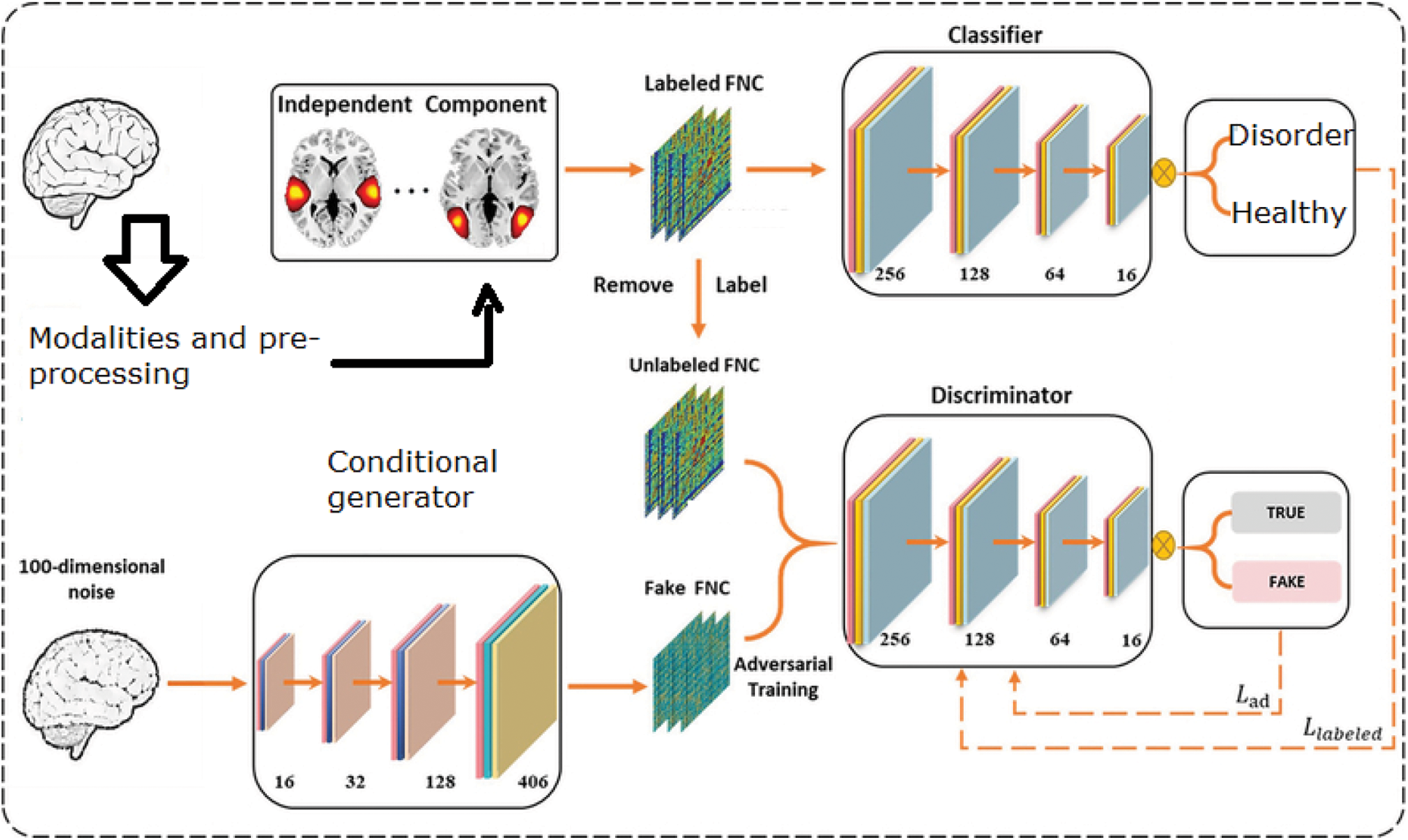
Figure 4: Conditional GAN architecture for ASD prediction
By providing a new objective loss, feature matching was able to solve GAN's instability and prevent it from overtraining on the discriminator. Instead of maximizing the discriminator's output directly, the new aim aids in the generation of data that matches the statistics of the real data, while the discriminator was simply employed to identify the statistics that were worth matching. The shape definition is invariant to the translation, scaling and rotation of the object in the learning system and, depending on the data, is expected to be either 2D or 3D. In general, it is difficult to accurately segment an image into important areas using low-level characteristics due to the variety of promising projections of a 3D object into 2D shapes, the complexity of each individual object shape, non-uniform illumination, the presence of shadows, occlusions, varying surface reflectivity.
Their shapes have to be defined, indexed, and compared after segmenting the region of interest. However, in the classification system, no detailed definition can completely capture all aspects of visually assumed shapes and shape comparison is also a very difficult problem. Not only does the restricted nature of the shape inhibit the systematic study of the trade-off between the ambiguity of the shape and the definition, but also its ability to define the shape of the picture as opposed to the shapes of interest. The generator was taught to match the feature value in the discriminator's intermediate layers. The third hidden layer is the intermediate layer we used in this investigation. Discriminative features can be discovered by training the discriminator using feature matching method, by the generator to differentiate actual data from produced data.
Two edge feature sets can be calculated by these edges in an 8 × 8 block:
where Hi and Vj correspond to the DCT coefficients Fu, v , for u, v = 0, 1, 2, …, 7, which describes the 2-dimensional DCT.
a) After that, the generator will attempt to calculate the (Euclidean) distance between the input image and the database images
b) The retrieved images are ranked according based on the distance measurement
c) The discriminator will distinguish between the input image and the retrieved images
d) The discriminator will then feedback the results to the discriminator to eliminate the false positives
e) The generator uses this feedback to retrieve a new set of samples from the database
f) The iteration stops when the discriminator could not feedback any results to the generator
Set of retrieved images that match to the input image. An image distance scale contrasts the resemblance of two images in different dimensions, such as color, texture, form, and others. For example, with respect to the dimensions that were considered, a distance of 0 implies an exact match to the question. A value greater than 0 implies different degrees of similarity between the images, as one can intuitively compile.
1. Different important features are extracted from the images in compressed domain rather than decoding and extracting
2. Generator training
3. Discriminator training
GANs employ a loss function that depicts the distance between the GAN-generated data distribution and the input data distribution.
The generator attempts to minimize the following function while the discriminator tries to maximize it in traditional GAN algorithms, which use the mini max loss function as:
Here
The discriminator's estimate of the probability that real data instance x is real is D(x).
Ex is the average of all real-world data cases.
When given noise z, the generator's output is G(z).
The discriminator's estimation of the probability that a fake instance is real is D(G(z)).
Ez is the expected value of all the generator's random inputs (in effect, the expected value of all generated fake instances G(z)). This can further be represented as:
Instead of using the traditional mini max loss function, we propose to use Wasserstein Loss function in our work. This function helps to better approximate the distribution of data observed in a given training dataset than the mini max loss function. In this loss function, Earth Mover's distance is used. This is calculated as:
Wasserstein distance can provide a meaningful and smooth representation of the distance between two distributions even when they are located in lower dimensional manifolds without overlaps. We maximize the probability assigned to the samples by the discriminator as:
An ideal training process for the proposed GAN system involves:
a) First, the generator will generate random images with simple distance measurements between the sensor image and the database images.
b) The discriminator network will learn with the help of basic filters to distinguish between the real images and random noise.
c) The generator will update the variable parameters present in the system including bias, threshold etc. to produce more images and confuses the discriminator.
d) The discriminator now becomes more attuned to real images matching to the sensor image and other noisy images and provides the feedback.
e) The process continues until the discriminator is maximally confused and no further feedback can be provided.
4.5 Novelty of the Proposed Work
1. GAN networks are not tried much for ASD prediction systems. So, this will be a new attempt to see the behaviour across different datasets.
2. Most GAN networks use only minimax loss function to replicate a probability distribution. So, the idea of using Wasserstein Loss function in GAN network for ASD prediction system can bring in better results than the existing systems.
3. A GAN will also have two loss functions, one for generator training and the other for discriminator training. So, we can try different combinations of loss functions (minimax vs. Wasserstein) to see which one behaves better for a given data set.
The three objective function responsible for the GAN learning process include the reconstruction loss, GAN loss and the Metric loss. The root mean square error between the input and output function refers to the reconstruction loss which penalizes the generator network for the differences introduced in it. It is formulated as:
where x corresponds to the original image and x refers to the generated output. The second loss is the GAN loss which is created for the better controlled training process. It is represented as:
where p(x|x) refers to the conditional distribution of the adversarial examples. The last loss function is the Metric loss which helps to push the examples away from the actual image along with its neighbours in the feature space. It is given by:
The complete loss function corresponds to the combination of three loss functions along with the proposed Wasserstein Loss function.
Four conventional techniques, SVM, Neural networks, Random Forest and a deep learning method (DNN), were utilized as a comparison in this study to evaluate the validity of the proposed conditional GAN approach. In layered 10-fold cross-validation cycles, the training and testing datasets were embedded. We utilized nine folds as the training set and one-fold as the testing dataset for all of the models. In the leave-one-site-out transfer classification, a specific imaging site was used as the testing set and a sample of other sites as the training set. The classification performance is measured by accuracy (ACC), sensitivity (SEN), specificity (SPE), F-score (F1), and area under curve (AUC).
Training and Testing requires big samples, yet single laboratories cannot acquire large enough datasets to show the brain processes causing ASD. As a result, the Autism Brain Imaging Data Exchange (ABIDE) project has gathered functional and structural brain imaging data from labs all around the world to help researchers better understand the neurological basis of autism. ABIDE 1 is a dataset of 1112 individuals, 539 of whom have ASD and 573 of whom are normal controls (ages 7–64 years, median 14.7 years across groups). ABIDE II comprises 19 locations, including 10 charter institutions and seven new members, who have together donated 1114 datasets from 521 people with ASD and 593 people who are not (in the age range of 5–64 years). We use this ABIDE dataset in our work to evaluate the performance of the proposed system.
In the ASD rs-fMRI data, the correlation between fMRI data for regions of the brain revealed two different groupings of areas that were negatively and positively correlated: First, a dispersed network of anterior and posterior brain regions with negatively associated rs-fMRI activity, and second is, a posterior network of areas with highly correlated rs-fMRI activation. The implications of these findings are explored in connection to an existing data-driven hypothesis of autistic brain anterior-posterior under connectivity.
The challenge is a binary classification job since the characteristics were collected from a population of healthy and autistic children. The goal is to identify autism using network measurements of EEG phase synchronized states. The paracingulate gyrus (Fig. 5a), supramarginal gyrus (Fig. 5b), and middle temporal gyrus (Fig. 5c) were the regions of the brain with the strongest anti correlation for ASD individuals as shown in Fig. 5 below. These areas' anti correlation patterns were the most important characteristics for our deep learning categorization.
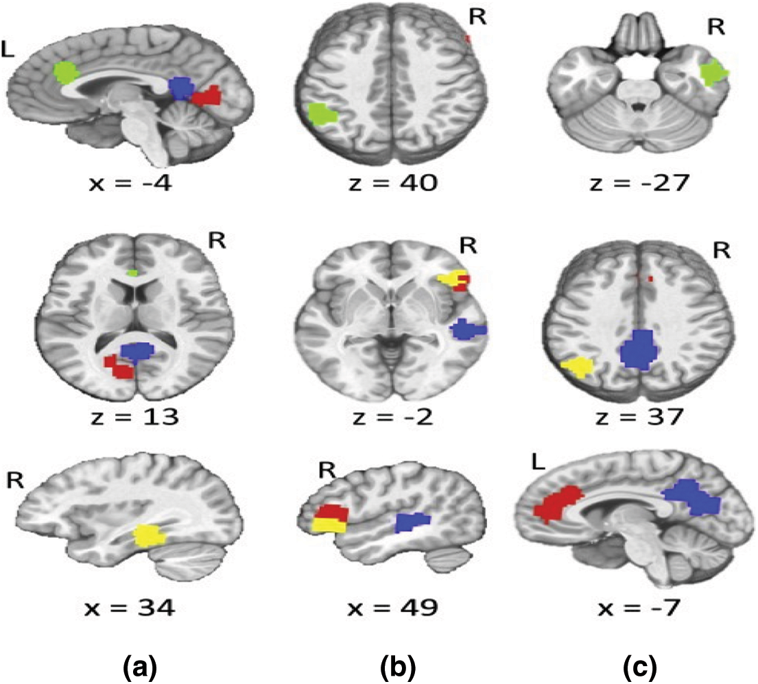
Figure 5: Sample video frame (left) and object detection (right) from the experimental data set
Our train/test split was 80/20, and the training set was partitioned into a training and validation set with an 80/20 ratio. We used an extended training dataset with random horizontal flips and ninety-degree rotations to train our end-to-end architecture. Our detection output came in the form of bounding boxes with associated classes. We used average precision (AP) to evaluate our results, and calculated intersection over union (IoU), precision, and recall to get AP. The collection of correctly recognized items is referred to as true positives (TP), while the set of incorrectly detected objects is referred to as false positives (FP). The precision is now calculated as the ratio of the number of TPs to all predicted objects:
The set of items that the detector does not detect is referred to as false negatives (FN). The recall is then calculated by dividing the number of detected items (TP) by the total number of objects in the data set:
The proportion of people who have the disease (as determined by the ‘Gold Standard’) who obtained a positive result on this test is referred to as sensitivity (True Positive Rate). The proportion of people who do not have the disease (as determined by the ‘Gold Standard’) who obtained a negative response on this test is referred to as specificity (True Negative Rate).
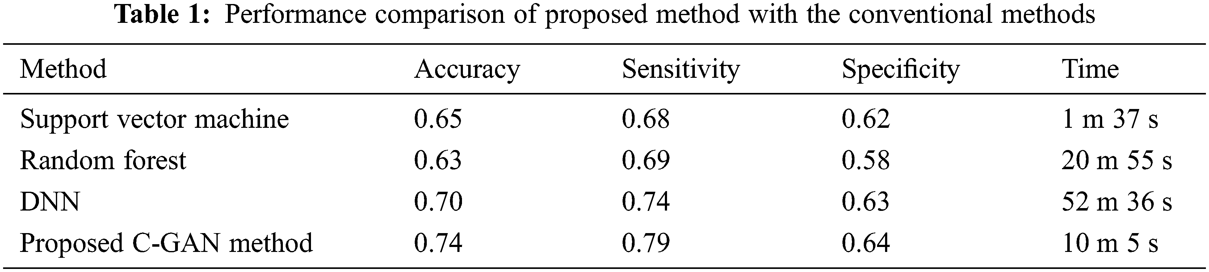
Sensitivity is a measure of how effectively a test can detect genuine positives, while specificity is a measure of how well a test can identify true negatives in a diagnostic test. There is typically a trade-off between sensitivity and specificity in all diagnostic and screening testing, with higher sensitivities implying lower specificities and vice versa. Tab. 1 below compares the accuracy, sensitivity and specificity along with the computation time for different classifiers including the support vector machine, Random Forest (RF), DNN and the proposed method.
Reduced anterior-posterior connection and enhanced local connectivity between posterior areas are characteristics of autism patients’ brain activity that have been replicated throughout our research. Fig. 6 below shows the comparison across methods in terms of accuracy, sensitivity and specificity parameters.
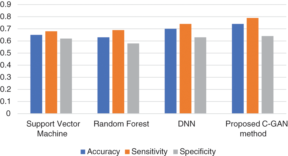
Figure 6: Accuracy, sensitivity and specificity across methods
Similarly, the time series comparison across different methods is shown in Fig. 7. It is evident from the experimentation results, that the proposed method is better in terms of accuracy, sensitivity and specificity parameters, while time taken for training needs some optimization when compared to existing methods.
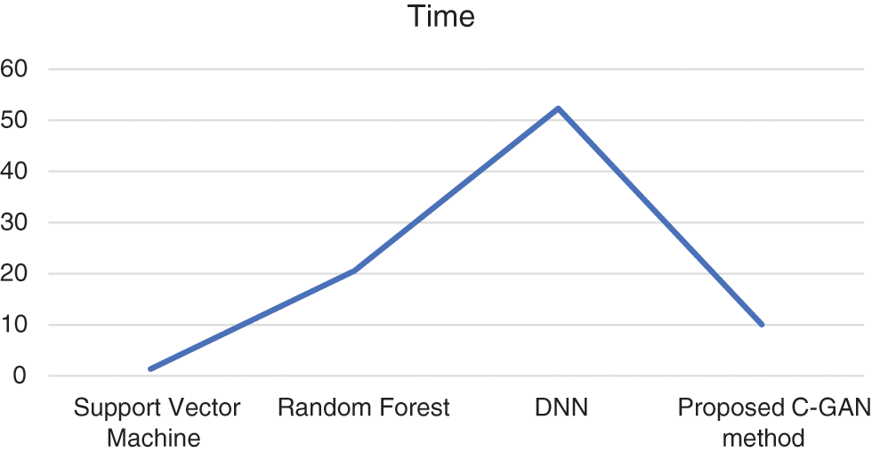
Figure 7: Training time across different methods
In comparison to previous research, the current study showed a substantial improvement in performance. Despite this, there are several restrictions that must be addressed. Only functional MRI data were used for classification, although a combination of functional and structural MRI data has been shown in published approaches to produce better prediction accuracy at the cost of longer training time. Other sophisticated neural network designs, such as CNN, 3D based CNN model, and others, can also be used for prediction and could be beneficial. However the existing results from our experiments proves that a diagnostic technique that combines machine learning algorithms with neuro images helps to distinguish ASD patients from healthy controls at very early stages.
Autistic Spectrum Condition is a disorder characterized by social interaction and communication problems due to genetic and neurological factors and in this work, we have discussed about using conditional generative adversarial networks for predicting ASD disorders in advance for timely treatment and to reduce the effects of Autism. Previous research on ASD brain function has shown that the disorder causes a breakdown in anterior-posterior brain connectivity, as well as an increase in posterior, or local, connectivity. The anticorrelation, we believe, represents a lack of connection between the anterior and posterior regions of the ASD brains, which are responsible for the majority of the current categorization. Deep learning algorithms like conditional generative adversarial networks discussed in this work are able to correctly identify large multi-site datasets, according to the findings. In compared to single-site datasets, classification over several sites might tolerate extra sources of variation in patients, scanning processes, and equipment. In the sense that new sequences maintain the original connections between variables throughout time, a suitable generative model for time-series data should retain temporal dynamics. Existing approaches for applying generative adversarial networks (GANs) to sequential data do not account for the temporal correlations that are specific to time-series data. The next goals of this research will be to generate realistic time-series data that blends the freedom of the unsupervised paradigm with the control provided by supervised training. Other imaging modalities, such as structural MRI data combined with functional MRI data, may offer additional information about ASD and be explored for review in future research.
Funding Statement: The authors received no specific funding for this study.
Conflicts of Interest: The authors declare that they have no conflicts of interest to report regarding the present study.
1. K. Shahrukh Omar, P. Mondal, N. Shahnaz Khan, M. Rezaul Karim Rizvi and M. Nazrul Islam, “A machine learning approach to predict autism spectrum disorder,” in Proc. Int. Conf. on Electrical, Computer and Communication Engineering (ECCE), Bazar, Bangladesh, pp. 1–6, 2019. [Google Scholar]
2. S. Ozonoff, K. Heung, R. Byrd, R. Hansen and I. H. Picciotto, “The onset of autism: Patterns of symptom emergence in the first years of life,” Journal of Autism, vol. 1, no. 6, pp. 320–328, 2010. [Google Scholar]
3. I. H. Sarker, “Machine learning: Algorithms, real-world applications and research directions,” Journal of SN Computer Science, vol. 2, no. 160, 2021. [Google Scholar]
4. L. A. Jorgenson, T. William and J. David Anderson, “The BRAIN initiative: Developing technology to catalyse neuroscience discovery,” Philos Transaction R Soc Lond B, vol. 2, no. 5, pp. 1–17, 2015. [Google Scholar]
5. B. M. Lake, T. D. Ullman, B. Joshua and J. Samuel, “Building machines that learn and think like people,” Journal of Behavioral and Brain Sciences, vol. 40, pp. e253, 2016. [Google Scholar]
6. J. Wolff, S. Jacob and J. T. Elison, “The journey to autism: Insights from neuroimaging studies of infants and toddlers,” Journal of Dev Psychopathol, vol. 30, no. 2, pp. 479–495, 2017. [Google Scholar]
7. M. Konnik, B. Ahmadi, N. May, J. Favata, Z. Shahbazi et al., “Training AI-based feature extraction algorithms, for micro CT images, using synthesized data,” Journal of Nondestructive Evaluation, vol. 40, no. 25, pp. 1–13, 2021. [Google Scholar]
8. J. Schmidt, M. R. G. Marques, S. Botti and M. A. L. Marques, “Recent advances and applications of machine learning in solid-state materials science,” NPJ Computational Materials, vol. 5, no. 1, pp. 1–36, 2019. [Google Scholar]
9. H. Zhang, “Image de-raining using a conditional generative adversarial network,” Journal of Computer Vision and Pattern Recognition, vol. 30, no. 11, pp. 3943–3956, 2019. [Google Scholar]
10. M. N. Parikh, L. Hailong and L. He, “Enhancing diagnosis of autism with optimized machine learning models and personal characteristic data,” Journal of Frontiers Computing and Neuroscience, vol. 13, no. 9, pp. 1–19, 2019. [Google Scholar]
11. W. Jamal, S. Das, I. Anastasia Oprescu, K. Maharatna, F. Apicella et al., “Classification of autism spectrum disorder using supervised learning of brain connectivity measures extracted from synchrostates,” Journal Neural Engineering, vol. 11, no. 4, pp. 46019–6032, 2014. [Google Scholar]
12. A. Azamimi Abdullah, S. Rijal and S. Ranjan Dash, “Evaluation on machine learning algorithms for classification of autism spectrum disorder (ASD),” in Proc. Int. Conf. on Biomedical Engineering, Penang island, Malaysia, vol.1372, pp. 26–27, 2019. [Google Scholar]
13. Q. Kong, B. Tong, M. Klinkigt, Y. Watanabe, N. Akira et al., “Active generative adversarial network for image classification,” in Proc. AAAI Conf. on Artificial Intelligence, Hong Kong, vol. 33, no. 1, pp. 4090–4097, 2019. [Google Scholar]
14. M. Rezaei, H. Yang and C. Meinel, “Generative adversarial framework for learning multiple clinical tasks,” in Proc. Digital Image Computing: Techniques and Applications (DICTA), Canberra, Australia, pp. 1–8, 2018. [Google Scholar]
15. B. Xiaan, Y. Wang, Q. Shu, Q. Sun and X. Qian, “Classification of autism spectrum disorder using random support vector machine cluster,” Journal of Frontier Genetics, vol. 9, no.18, pp. 18–28, 2018. [Google Scholar]
16. S. Jebapriya, S. David, J. W. Kathrine and N. Sundar, “Support vector machine for classification of autism spectrum disorder based on abnormal structure of corpus callosum,” International Journal of Advanced Computer Science and Applications, vol. 10, no. 9, pp. 10–14569, 2019. [Google Scholar]
17. Z. Sherkatghanad, M. Akhondzadeh, S. Salari, M. Zomorodi, M. Abdar et al., “Automated detection of autism spectrum disorder using a convolutional neural network,” Journal of Frontier Neuroscience, vol. 13, pp. 1325. 2020. [Google Scholar]
18. A. Heinsfeld, A. Rosa Franco, R. CameronCraddock, A. Buchweitz and F. Meneguzzi, “Identification of autism spectrum disorder using deep learning and the ABIDE dataset,” Journal of NeuroImage: Clinical, vol. 17, pp. 16–23, 2018. [Google Scholar]
19. J. Song, N. Yoon, S. M. Jang, G. Young Lee and B. Nyun Kim, “Neuroimaging based deep learning in autism spectrum disorder and attention deficit hyperactivity disorder,” Journal of the Korean Academy of Child and Adolescent Psychiatry, vol. 31, no. 3, pp. 97, 2020. [Google Scholar]
20. W. Yin, S. Mostafa and F. Xiang, “Diagnosis of autism spectrum disorder based on functional brain networks with deep learning,” Journal of Computing Biology, vol. 28, no. 2, pp. 146–165, 2021. [Google Scholar]
 | This work is licensed under a Creative Commons Attribution 4.0 International License, which permits unrestricted use, distribution, and reproduction in any medium, provided the original work is properly cited. |