DOI:10.32604/csse.2023.025390
| Computer Systems Science & Engineering DOI:10.32604/csse.2023.025390 | |
| Article |
Twitter Data Analysis Using Hadoop and ‘R’ and Emotional Analysis Using Optimized SVNN
Department of CA, M S Ramaiah Institute of Technology, 560054, Bangalore, India
*Corresponding Author: K. Sailaja Kumar. Email: sailajakumar.k@gmail.com
Received: 22 November 2021; Accepted: 11 January 2022
Abstract: Standalone systems cannot handle the giant traffic loads generated by Twitter due to memory constraints. A parallel computational environment provided by Apache Hadoop can distribute and process the data over different destination systems. In this paper, the Hadoop cluster with four nodes integrated with RHadoop, Flume, and Hive is created to analyze the tweets gathered from the Twitter stream. Twitter stream data is collected relevant to an event/topic like IPL- 2015, cricket, Royal Challengers Bangalore, Kohli, Modi, from May 24 to 30, 2016 using Flume. Hive is used as a data warehouse to store the streamed tweets. Twitter analytics like maximum number of tweets by users, the average number of followers, and maximum number of friends are obtained using Hive. The network graph is constructed with the user’s unique screen name and mentions using ‘R’. A timeline graph of individual users is generated using ‘R’. Also, the proposed solution analyses the emotions of cricket fans by classifying their Twitter messages into appropriate emotional categories using the optimized support vector neural network (OSVNN) classification model. To attain better classification accuracy, the performance of SVNN is enhanced using a chimp optimization algorithm (ChOA). Extracting the users’ emotions toward an event is beneficial for prediction, but when coupled with visualizations, it becomes more powerful. Bar-chart and wordcloud are generated to visualize the emotional analysis results.
Keywords: Twitter; apache Hadoop; emotional analysis; OSVNN; ChoA; timeline graph; flume; hive
The amount and type of data generated by Online Social Networks (OSNs) OSNs provide challenges and opportunities for data storage and analysis [1,2]. Methods for evaluating OSNs structures to find prominent actors, local and global trends, and network dynamics are covered in the investigation of network architectures [3]. OSNs have experienced unique scalability, management, and maintenance problems due to their exceptional growth and popularity. As OSNs become increasingly larger and more powerful, they are subject to new challenges, more importantly scalability. The ability of a system to expand its performance under greater demand is known as scalability. Designers of OSNs are forced to decide whether to apply best practices and build scalable OSNs for a potential success that may never materialize or follow best practices and build fully-featured OSNs that require a high level of time and resources. Scaling up without a plan is a dangerous strategy, especially for OSNs with rapid growth potential. Processing OSNs with hundreds of millions of edges can be challenging in a single machine, according to [4]. The single-server memory method is large enough to store the whole un-partitioned social network, reducing the redundancy of some of the partitioned models. This is more efficient on many levels, but it is more expensive due to the necessity to fit the complete social network into a single server’s memory. In a scalable network, adding nodes does not degrade the performance, and the throughput remains consistent regardless of the number of nodes [5]. In addition, the scalable social network must retain the response and latency time irrespective of the amount of content added or the number of users connecting simultaneously. According to the survey [6], OSNs are divided into centralized, decentralized, and hybrid architectures. Several scalability metrics were used to compare the architectures, such as availability, latency, inter-server communication, resource costs, energy consumption, etc. In addition, several scalability difficulties faced by these categories, such as handling a huge volume of users, network resource management, information dissemination and storage, and energy consumption, have been thoroughly examined [7–9].
Twitter real-time data is scaling up from Gigabyte, Terabyte to Petabytes. Managing and processing Twitter data and the interactions of users using a single machine is a significant challenge. Handling the dynamic information created by Twitter users is a major problem. Because of the exponential expansion of Twitter users, failing to incorporate scalability into the original design of the Twitter network can be fatal. For instance, in addition to the usual growth rate, Twitter saw an increase of 1,382% in the period of one year, February 2008 to February 2009 [10]. In its continuous growth, Twitter has been plagued with significant downtime due to its inadequate infrastructure to handle the huge volume of traffic generated by its growing user base. As a result, Twitter’s architecture was completely revamped [11]. Similarly, to accommodate the enormous growth of users, MySpace3 engineers had to revamp their Web-based apps, databases, and data storage systems.
Facebook recently added geo-replication support. In this case, one large-scale geo-redundancy service is implemented by adding an east coast data center both for East Coast users’ convenience and to ensure redundancy for the west coast site. It has many benefits; however, it becomes more challenging if no clean partition of the Facebook user ID is available. Scalable computing systems must retain consistent performance with increased workloads [12]. Researchers have proposed parallel processing environments, Apache Hadoop framework, MapReduce programming model, programming languages’ R’ and Python to address the scalability issues associated with Twitter data [13]. As well as, they prefer Flume to extract or collect the real time twitter data and store in the centralized stores such as Hadoop Distributed File System (HDFS) and Hbase. It makes easy to analyze the collected twitter data.
This paper addresses the scalability issues by constructing a Hadoop cluster with a single node, then scaling it up to four nodes to process Twitter streaming data. This research describes how Twitter users behave on social networks by understanding their behavior and visualizing various statistics using ‘R’ and Apache Hadoop data analysis tools. Twitter generates gigabytes of data each day, and it must be distributed among multiple systems because each system has memory limitations. Apache Hadoop, which comes with HDFS, distributes data around the systems. Data obtained from Twitter will be in raw JavaScript Object Notation (JSON) format and contain many Twitter attributes, so it will need to be processed before further analysis can be conducted. Hive is a data warehouse infrastructure tools that stores and processes raw data available in HDFS. Besides, this paper focuses on emotional analysis of users to predict future events.
Contributions of the paper are given as follows,
• Twitter analytics like the maximum number of tweets by users, the average number of followers, users with the maximum number of friends are obtained using Hive.
• The network graph is constructed with the user’s unique screen name and mentions using ‘R’. A timeline graph of individual users is generated using ‘R’.
• Also, the proposed solution analyses the emotions of cricket fans by classifying their Twitter messages into appropriate emotional categories using OSVNN classification model. In the proposed classification model, ChOA algorithm is used to optimize the weight parameters of SVNN. Automatically extracting the users’ emotion toward an event/ object is very important for prediction, but when coupled with visualizations, it becomes more powerful.
• Bar-chart and wordcloud are generated to visualize the emotional analysis results.
The remaining sections of the article are sorted as follows. The recent works of literature which focused research on emotion analyses are reviewed in Section 2. Section 3 describes the system architecture and analysis of the emotion of cricket fans using OSVNN. Experimental results of the proposed methodology are discussed in Section 4. The conclusion of the paper is described in Section 5.
In this section, emotion analysis-based recent research works are reviewed. Hasan et al. [14] had introduced a soft classification scheme to estimate the probability of message to every class of emotion. Besides they had developed a supervised learning framework for emotion classification. In the approach, emotions in text messages were classified in the model of the offline training task. Also, real-time emotions in text messages were classified in the model of the online training task. Stojanovski et al. [15] had analyzed various pre-trained classifiers and word embeddings combined with the convolutional neural network. The proposed model was applied to different schemes such as sentiment analysis and identification of emotion. Abdi et al. [16] had introduced the Auxiliary Dataset-Latent Dirichlet Allocation scheme for enhancing the user’s emotions learning in a particular topic. In the model, emotions were considered as predefined sentiments. Yan et al. [17] had considered sparseness, ambiguities, and non-standardization in a subject of short texts for emotion classification. Besides, the authors had introduced a low-dimensional hybrid feature model, as well as they, had presented the emotion-improved inference model which included a set of fuzzy reasoning rules.
Prasanna et al. [18] had introduced neuro-fuzzy structure-based phrase-level emotion patterns. In the approach, the patterns were extracted at the level of phrase and converted into fuzzy rules for emotion classification. The patterns were classified as negative and positive emotions using an intensity grade which was measured phrase features and sentence structure. For emotion detection, Ghanbari-Adivi et al. [19] had introduced an ensemble classifier which was developed based on the basic classifiers such as decision tree, k-nearest neighbor, and multilayer perceptron. The performance of the proposed classifier was enhanced by optimizing the tuning parameters of basic classifiers using Tree-structured Zhang et al. [20] had introduced a multiple emotions detection scheme in online social networks. Initially, the authors had estimated the correlations of social, temporal, and emotion labels from the Twitter dataset. Depending on the correlations; the authors had developed the emotion detection structure based on a factor graph. At final, multiple emotions were detected depending on the multi-label learning scheme. From the above works of literature, we conclude that the classification accuracy for emotion analysis is further to be enhanced. To attain this goal, an enhanced hybrid machine learning technique is presented in this paper. Also this study focuses to predict the future events in terms of the users emotions.
3 System Architecture and Methodology
System architecture presented in Fig. 1 is used for analyzing the Twitter data. It consists of a Hadoop cluster with a supportive eco-system. Real-time stream data is fetched from Twitter using the Flume agent with a particular keyword and saved to HDFS in JSON format. Twitter data is loaded into the Hive data warehouse and analyzed using the Hive Query Language. Hadoop and ‘R’ are used to preprocess the data and generate visual graphs.
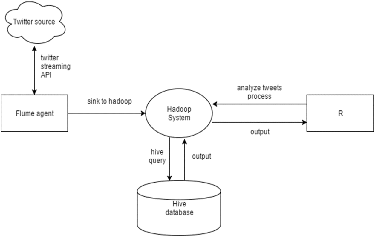
Figure 1: System architecture
The methodology to analyze the Twitter data using Hadoop, Hive, and ‘R’ is given below. The methodology is used to analyze Twitter users’ behavior and visualize the various statistics with the help of graphs.
• Using apps.Twitter.com create a Twitter account.
• Twitter credentials are authenticated to obtain the data from Twitter.
• Hadoop cluster is created with RHadoop and Flume.
• Fetch Twitter real-time stream data using Flume agent and save the raw data in JSON file to HDFS.
• Store the JSON data in a structured columnar fashion using Hive.
• Fetch the required data from the Hive tables using Hive Queries.
• Load the tweets and load the relevant packages of R for tweet preprocessing.
• Extract the user’s unique screen name, and user mentions to construct the network graph.
• Construct the timeline graph of individual users.
• Perform emotion analysis using the OSVNN based on R’s syuzhet package and visualize the emotion scores using a bar chart.
• Construct wordcloud to depict the words in the tweets that are associated with the event.
3.3 ‘R’ and Hadoop Integration Process
RHadoop, provided by Revolution Analytics, is an open-source solution for ‘R’ and Hadoop. Integrating ‘R’ with Hadoop helps scale ‘R’ program to work with petabyte data. This integration extracts tweets from Twitter and stores them in HDFS for further processing [21]. The packages available in RHadoop manage and analyze the data with the ‘R’ and Hadoop frameworks.
The RHadoop packages used to stream tweets from Twitter are:
• rhdfs: provides access to HDFS installed on the name node where the ‘R’ code runs, allowing the user to browse, read, write and edit the files in HDFS
• plymr: is used to perform data manipulation operations on data stored on every node in Hadoop Cluster
• rmr2: supports statistical analysis in ‘R’ via Hadoop MapReduce functionality on every node in Hadoop Cluster
• rhbase: is used to integrate the ‘R’ database management capability with HBase
• rJDBC: enables basic connectivity to the database using JDBS Driver and installed on the node that runs the ‘R’ code.
3.4 Extracting the Tweets from Twitter Using Flume Agent
Tweets related to Modi, IPL 2015, cricket, (Royal Challengers of Bangalore) RCB, Kohli for May 24, Tuesday 6:49 2016 to May 30 Monday 12:22 2016 are extracted using RHadoop and Flume. Flume is used for streaming real-time data from Twitter. Flume Agent fetches the live stream from Twitter using the Twitter credentials and stores the streamed data in HDFS in raw JSON format. Real-time Twitter data related to the specific topic/keyword is extracted using the Flume Agent in a raw JSON file. The real stream data is fetched using the Flume Agent from Twitter by making the handshake to the Twitter server giving the Twitter user credentials. Flume agent creates multiple individual files and stores them at different nodes. These files contain the raw unprocessed JSON formatted tweets and the sample tweets in JSON format.
3.5 Twitter Analytics Using Hive
Hive is used as a data warehouse to store the streamed tweets. Twitter JSON data is stored in HDFS, and it is extracted and loaded into the Hive data warehouse. Further, the Twitter data is analyzed using HQL. It is used to extract the Hive tables and the records available in a particular table.
3.6 Twitter Data Visual Analysis Using ‘R.’
RStudio, an interactive (Graphical User Interface) GUI tool for ‘R’, is installed to analyze the Twitter data. ‘R’ stores the data on RAM. Since the RAM and hard disk spaces are limited, ‘R’ and Hadoop are integrated to improve efficiency. The Twitter data obtained using Apache Flume is given input to ‘R’ to process in parallel and produces a single output for the same data.
As a result of the popularity of IPL on Twitter, Twitter also provides official hashtags (#IPL, #IPL2015) to promote the game. The proposed solution analyses the emotions of cricket fans by classifying their Twitter messages into appropriate emotional categories using the OSVNN model. The extracted Twitter sentiment packages of the R library are given as input to the proposed OSVNN. Using the proposed OSVNN model, the emotions of cricket fans such as happy, fear, sad, and anger are categorized.
SVNN: In SVNN classifier, the Support Vector Machine (SVM) is integrated with Artificial Neural Network (ANN). The SVNN model includes three layers such as input layer, hidden layer, and output layer. The SVM classifier is performed in the output layer. The input and hidden layer’s neuron size and the number of features are idle. The input layer and hidden layers are connected using weight values. The structure of SVNN is given in Fig. 2. And each step of detection is given below;
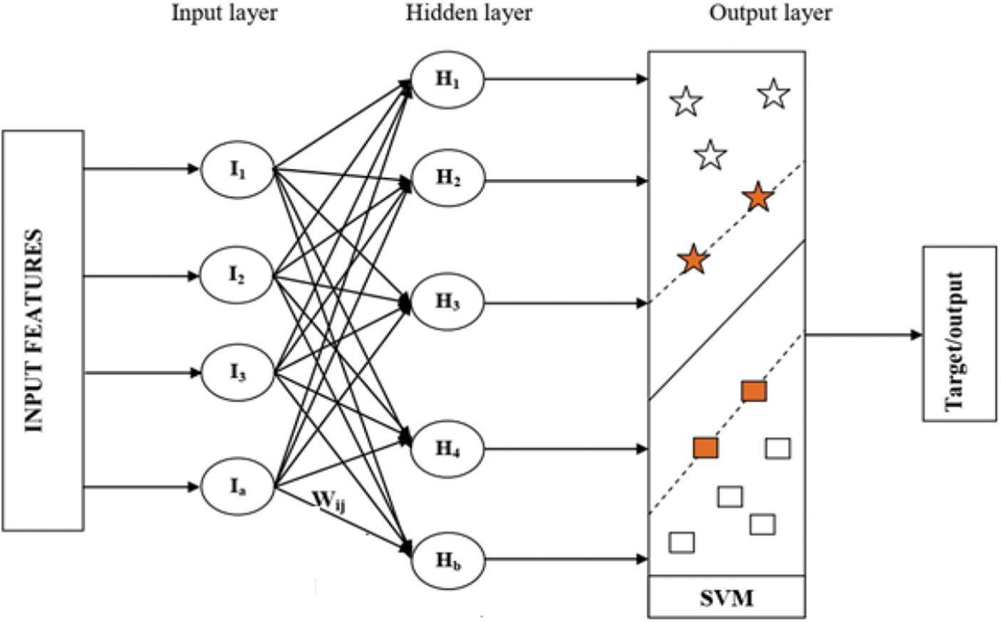
Figure 2: Structure of SVNN
Step 1: Initially, the selected features (inputs) are given to the ANN input layer. In the ANN, the input layer neuron is represented as
Step 2: The input value is multiplied with the corresponding weight value to obtain the hidden layer output. The mathematical function of hidden layer output is calculated as follows;
where, Bias value is defined as
Step 3: Once we obtained the hidden layer output, the activation function is applied on Hj. The mathematical function is given as follows;
Step 4: Then, the output of the hidden layer is transferred to the SVM. In SVNN model, the SVM acts as the output layer. An important characteristic of SVM is that it simultaneously reduces the experience classification error and increases the geometric margin. SVM maps the input data to the high-dimensional feature area, where it creates a hyperplane that separates the data.
Consider the data points
where; B is defined as the threshold and
where,
C1 → Bias value of the hidden layer
C2 → Bias value of output layer
After the output, the error is calculated. The error is evaluated between output and target value. In this paper, the error is calculated using Eq. (5).
where, the number of features is defined as N, OClass is defined as obtained output, OTaris defined as the target value,
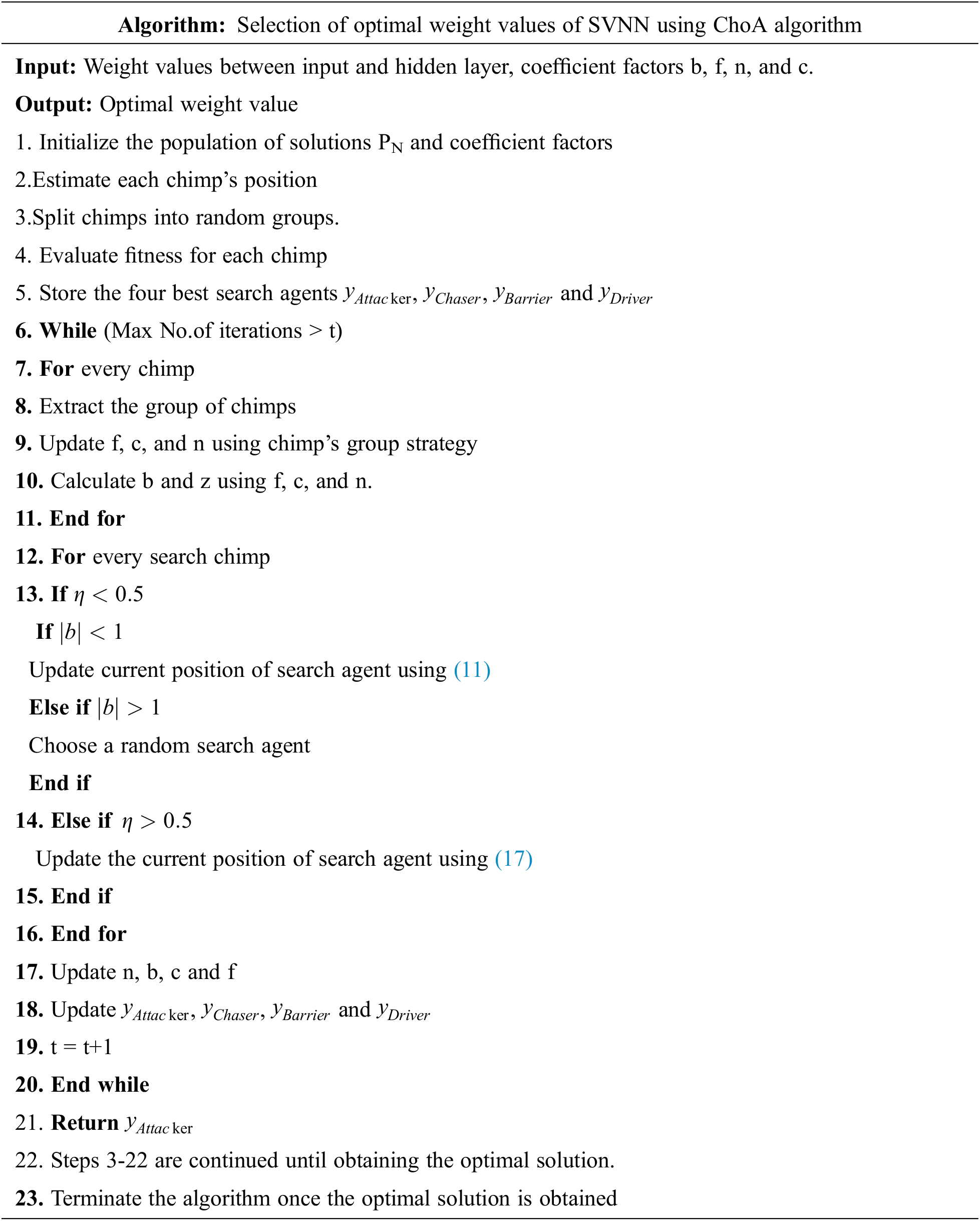
OSVNN: In this section, the performance of SVNN is improved by optimizing the weight values it using ChOA algorithm. In this algorithm, chimps are African species of great ape and are also known as Chimpanzees. In a chimp’s colony, every group of chimps autonomously endeavors to find the hunt space with its technique. In every group, chimps are not exactly comparable as far as ability and knowledge; however, they are all performing their responsibilities as an individual from the colony. The ability of every individual can be helpful in a specific circumstance.
Besides, the chimp colony has four kinds of chimps those are described as follows,
• Drivers: They only pursue the prey but do not try to catch it.
• Barriers: They place themselves in a tree to assemble a dam across the movement of the prey.
• Chasers: They follow quickly after the prey to hunt it
• Attackers: They guess the prey’s breakout route to turn it back towards the chasers or down into the lower shelter.
In general, chimp’s hunting process is partitioned into two fundamental stages: “Exploration” which comprises driving, impeding, and pursuing the prey, and “Exploitation” which comprises assaulting the prey
Initialization: In ChOA, the position of the chimps represents the position of the solutions in the search space. In this work, weight values between the input and hidden layer of SVNN are considered as the solutions. The population of the solutions is initialized as follows,
where, yN denotes the Nth solution or the position of the chimp and it can be represented using (7).
Here, wij denotes the weight value between ithinput layer and jth hidden layer.
Fitness Calculation: The fitness of every solution is estimated using accuracy. It can be defined using (8).
Here, the accuracy is calculated using (9).
Here, TP and FP denote true positive and false positive respectively and TN and FN denote true negative and false negative respectively.
According to (8), the solution or the solution with maximum fitness is chosen as optimal weight values. In this algorithm, the position of the optimal solution denotes the position of the prey. If the desired fitness is not obtained, the solution is updated based on the hunting behavior of chimps.
Update the solution: The following phases explain the hunting process of chimps or updating of solution.
Driving and Chasing the Prey: The mathematical expression of driving and chasing the prey is defined in Eqs. (10) and (11).
where, t denotes the current iteration, the position of prey is denoted as yprey, and the position of chimp is denoted as ychimp. b, c and n denote the coefficient vectors and are determined as follows,
where,
Exploitation or attacking stage: In the hunting process, driver, barrier, and chaser chimps support the attacker chimps to hunt the prey. Generally, the process of hunting is executed by the attacker chimps. In the mathematical expression, the location of the prey is identified from the best solution or first attacker, driver, barrier, and chaser. The attained four best solutions are stored. Then, depending on the location of the best chimps, the positions of other chimps are updated. This can be defined in Eqs. (15)–(17).
Prey attacking stage: In this stage, the prey will be attacked by the chimps and the hunting process is stopped as the prey stopped its movement. A chimp chooses its next position between the prey’s position and its current position when the value of b lies within [–1, 1]. The chimps are forced to attack the prey if
Exploration stage: In this stage, the chimps are diverged from the prey and are forced to search for the best prey. The chimps are forced to find the best prey
Social motivation: In this stage, the chaotic maps have been utilized to enhance the execution of ChOA. These chaotic maps are deterministic cycles that likewise have random behaviors. To demonstrate this concurrent behavior, we expect that there is a likelihood of half to pick between either the ordinary updating position method or the chaotic model to update the chimps’ position. The mathematical expression of the behavior is defined in Eq. (18).
where,
Termination: The solutions are updated based on the hunting behavior of chimps until attaining the optimal solution or best weight values. Once the solution is obtained, the algorithm will be terminated.
In the testing phase, the trained OSVNN model is executed based on the Twitter sentiment package of R. From the output of OSVNN, the emotions are classified i.e., if the output value is 0.5, emotion is happy, 1-sad, 1.5-fear, and 2-anger.
As a result of the proposed system, cricket fans can understand their fine-grained emotions rather than their sentiments, which are mainly coarse-grained. Automatically extracting the users’ emotion toward an event/ object is very important for prediction, but when coupled with visualizations, it becomes more powerful.
The proposed scheme is simulated in the platform of Python. The twitter dataset is collected using API. As shown in Fig. 3, the Hadoop cluster is created with four nodes to extract and analyze tweets. It consists of one name node and three slave nodes to store and process the tweets. Network community graph is generated as shown in Fig. 4a. It shows the network of the Modi community with others. The network graph presented in Fig. 4b shows the interaction of various communities associated with IPL. Also, the network of one community with others, considering more than 100,000 tweets, is shown in Fig. 4c. Further, the timeline graph on IPL data is generated as given in Fig. 4d. Wordcloud for the IPL tweets isgenerated, as shown in Fig. 5. Fig. 6a shows the result of the emotional analysis of IPL data as a bar chart. An emotional analysis result illustrating RCB’s loss during the IPL is given in Fig. 6b.
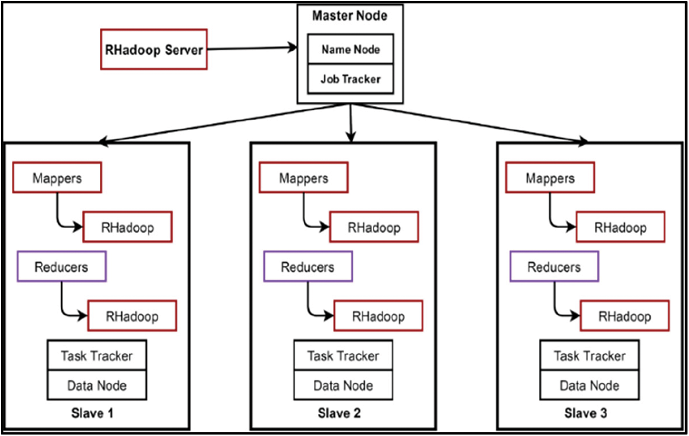
Figure 3: Hadoop cluster
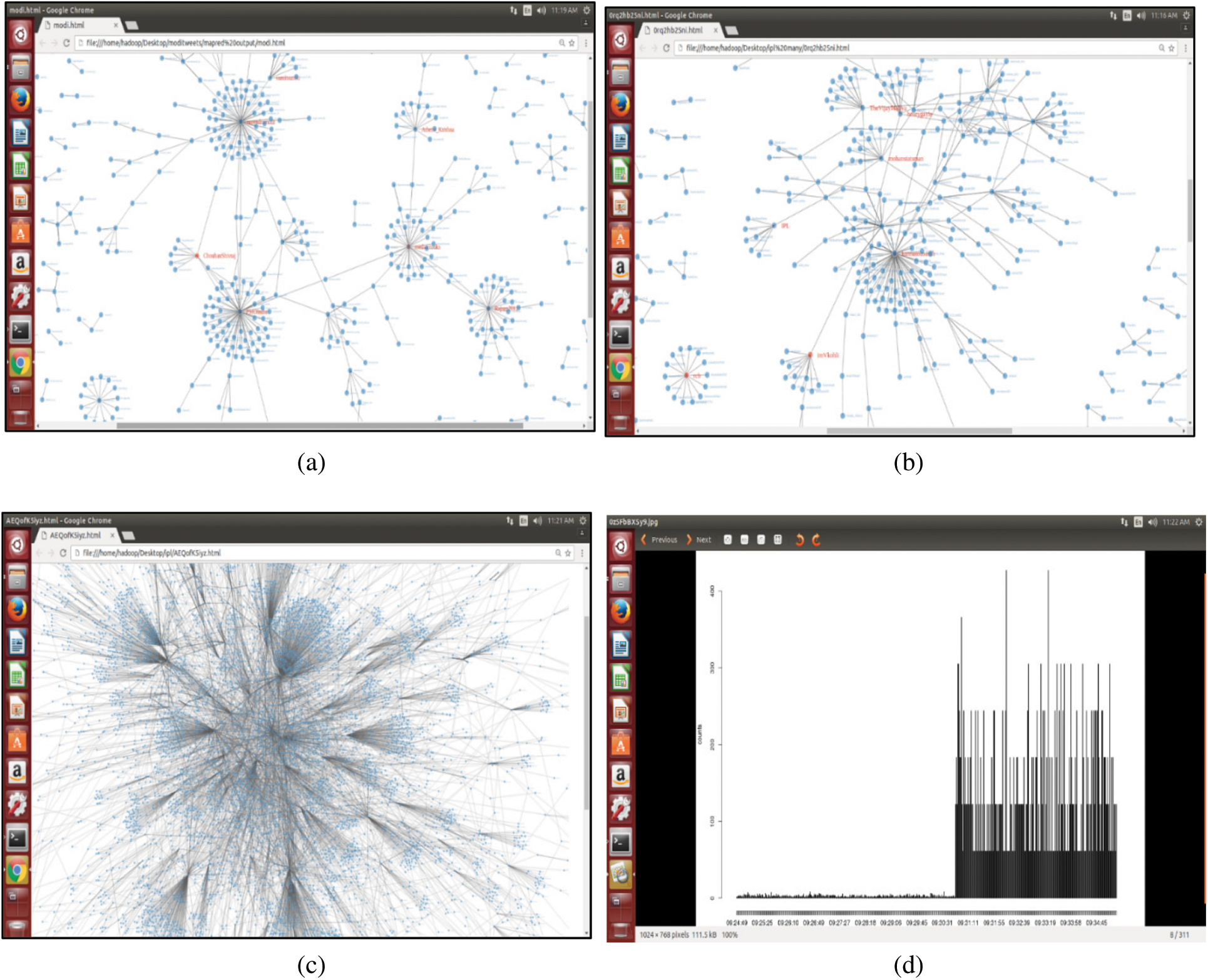
Figure 4: a) Modi tweets with maximum reducers b) IPL tweets network graph c) IPL tweets network with minimum reducers d) Timeline graph on IPL
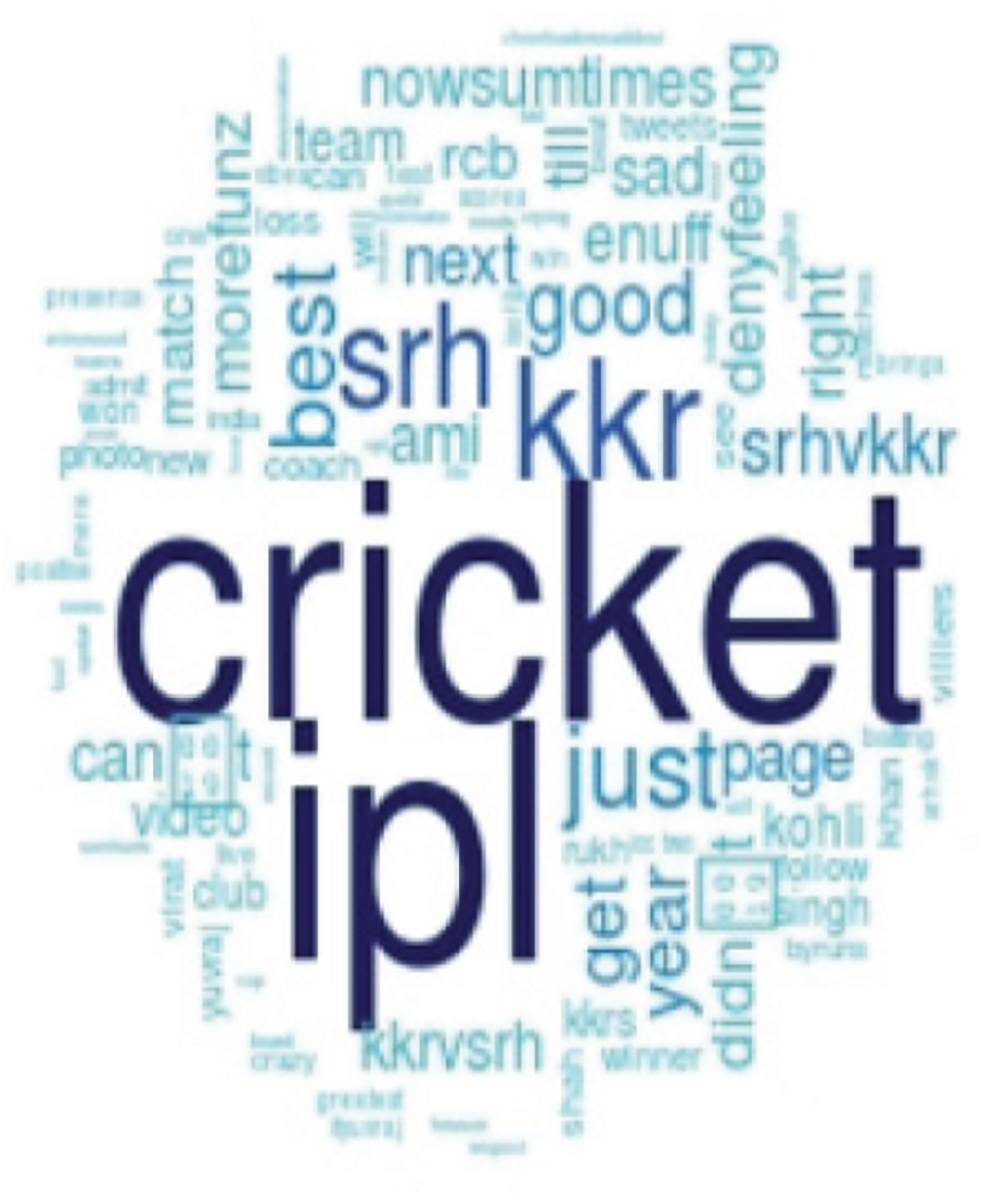
Figure 5: IPL tweets wordcloud
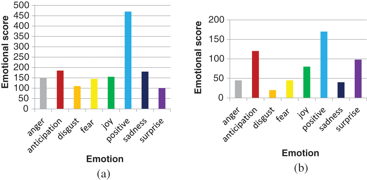
Figure 6: a) Emotion graph on IPL b) Emotion graph on IPL when RCB lost
4.2 Performance Analysis for Emotion Classification
In this section, the performance of different classification models is evaluated and compared in terms of accuracy, sensitivity, specificity, and F-measure. From the clustered twitter data, emotions of users are categorized using different classification models. Tab. 1 shows the performance analysis of different classification models. As shown in the table the performance of the proposedChOA-SVNN model is compared with that of the SVNN, SVM, ANN and random forest (RF). Fig. 7a illustrates the comparison of the accuracy of different classification models. As depicted in the figure, the SVNN based segmentation model attained 94% of accuracy than the SVM, ANN, and RF. However, by optimizing the weight values between the input and hidden layer ofSVNN using ChOA, the accuracy of ChOA-SVNN is increased to 97% than that of SVNN. The sensitivity of the proposed classification model is analyzed in Fig. 7b. As illustrated in the figure, the existing classification models such as SVNN, SVM, ANN, and RF attained 95%, 92%, 91%, and 51% of sensitivity respectively. Nevertheless, compared to these segmentation models, the proposed ChOA-SVNN based classification model attained 98% of sensitivity. Fig. 7c depicts the specificity of the different classification models. Compared to SVM, ANN, and RF, the SVNN based classification model attained 99% of specificity. The Fig. 7d depicts the comparison of the F-measure of different classification models. As depicted in the figure, the proposed ChoA based SVNN model attained 98% of classification accuracy than the existing classification models.
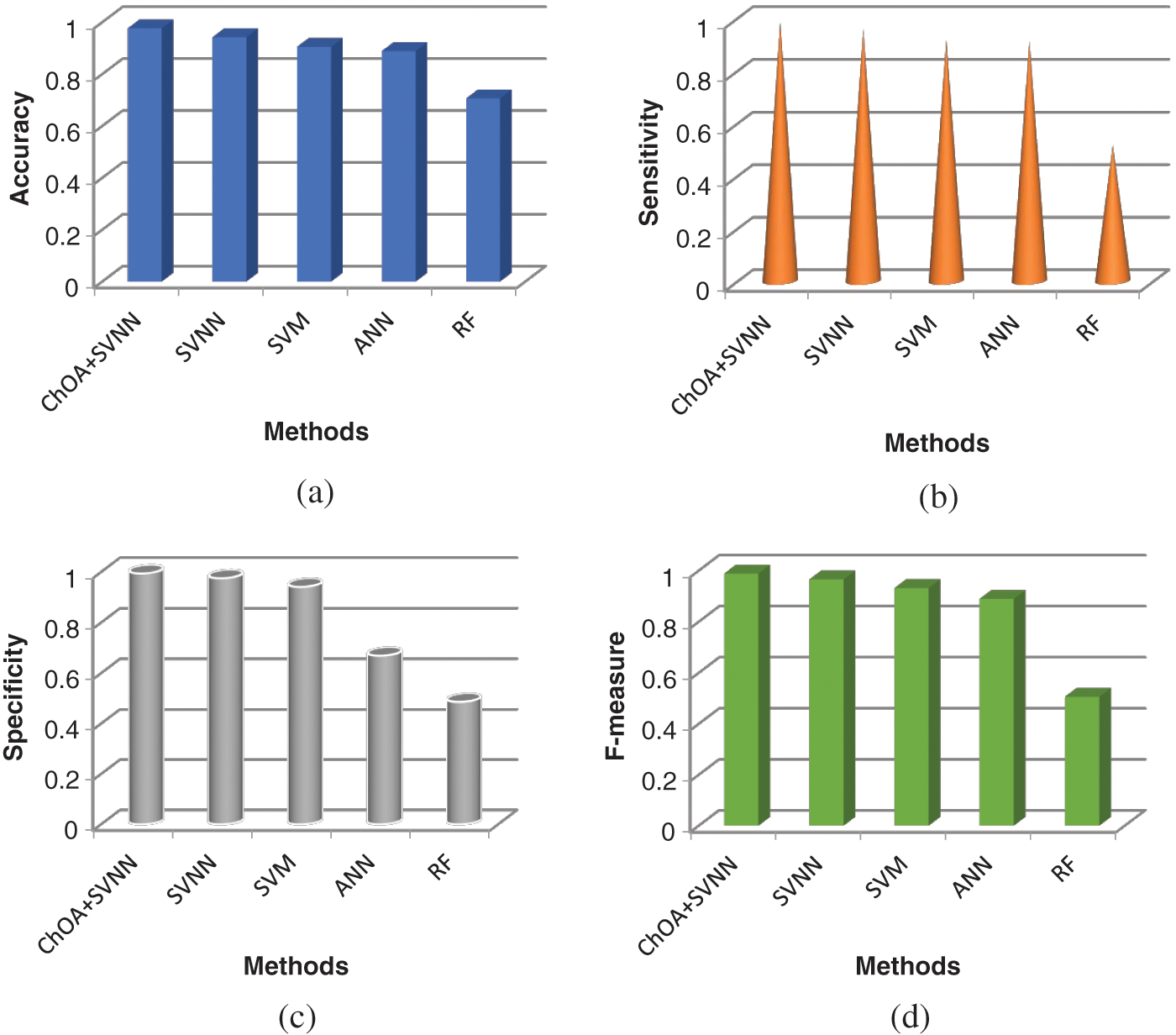
Figure 7: a) Accuracy b) Sensitivity c) Specificity d) F-measure
Twitter real-time data is scaling up from Gigabyte, Terabyte to Petabytes. In general, scaling up is a difficult exercise, and however, it is particularly challenging for Twitter because of its potential for rapid growth. In this paper, the Hadoop cluster integrated with RHadoop, Hive, and HBase is created to analyze the tweets gathered from the Twitter stream. The Twitter data stream is captured using Apache Flume. HBase and Hive Queries extract the Twitter users with maximum tweets count, average followers, and maximum friends. Twitter users’ network graph and timeline graph of the individual user are generated using RHadoop. Depending on the RHadoop package, emotions of cricket fans are classified using ChOA based SVNN model where weight parameters between input and hidden layer are optimized using ChOA. Based on the emotions, charts are developed to visualize the Twitter users’ emotional analysis using RHadoop. Data scalability issues are plenty on OSNs. In the present framework, Twitter real-time stream data is gathered using Flume and processed using the Hive and ‘R’. In the future, the existing Hadoop cluster can be extended with additional nodes to handle streaming data more efficiently. This may be enhanced with Apache Spark, which is quicker than MapReduce due to its in-memory data processing capabilities. Besides, automatic emotion recognition will be presented using enahnced deep learning techniques.
Acknowledgement: The author with a deep sense of gratitude would thank the supervisor for his guidance and constant support rendered during this research.
Funding Statement: The authors received no specific funding for this study.
Conflicts of Interest: The authors declare that they have no conflicts of interest to report regarding the present study.
1. L. Garton, C. Haythornthwaite and B. Wellman, “Studying online social networks,” Journal of Computer-Mediated Communication, vol. 3, no. 1, pp. 0–10, 2006. [Google Scholar]
2. A. Wolfe, “Social network analysis: Methods and applications,” American Ethnologist, vol. 24, no. 1, pp. 219–220, 1997. [Google Scholar]
3. W. Stanley and F. Katherine, “Social network analysis in the social and behavioral sciences,” in Social Network Analysis: Methods and Applications. Cambridge: Cambridge University Press, pp. 1–27, 1994. [Google Scholar]
4. http://perspectives.mvdirona.com/2008/06/08/ScalingLinkedIn.aspx. [Google Scholar]
5. T. Maqsood, O. Khalid, R. Irfan, S. Madani and S. Khan, “Scalability issues in online social networks,” ACM Computing Surveys, vol. 49, no. 2, pp. 1–42, 2016. [Google Scholar]
6. B. Pang, L. Lee and S. Vaithyanathan, “Thumbs up? sentiment classification using machine learning techniques,” EMNLP ’02: Proc. of the ACL-02 Conf. on Empirical Methods in Natural Language Processing, vol. 10, pp. 79–86, 2002. [Google Scholar]
7. J. Ugander, B. Karrer, L. Backstrom and C. Marlow, “The anatomy of the facebook social graph,” arXiv preprint arXiv:1111.4503, 2011. [Google Scholar]
8. C. Aggarwal, “An introduction to social network data analytics,” in Social Network Data Analytics. Boston, MA: Springer, pp. 1–15, 2011. [Google Scholar]
9. A. Alajlan and K. Elleithy, “High-level abstractions in wireless sensor networks: Status, taxonomy, challenges, and future directions,” in Proc. of the 2014 Zone 1 Conf. of the American Society for Engineering Education, Connecticut, U.S.A, pp. 1–7, 2014. [Google Scholar]
10. T. Sakaki, M. Okazaki and Y. Matsuo, “Earthquake shakes twitter users: real-time event detection by social sensors,” in Proc. of the 19th Int. Conf. on World Wide Web, North Carolina, USA, pp. 851–860, 2010. [Google Scholar]
11. J. M. Pujol, V. Erramilli, G. Siganos, X. Yang, N. Laoutaris et al., “The little engine (S) that could: Scaling online social networks,” ACM SIGCOMM Computer Communication Review, vol. 41, no. 4, pp. 375–386, 2011. [Google Scholar]
12. S. T. Chakradhar and A. Raghunathan, “Best-effort computing: re-thinking parallel software and hardware,” in Proc. of the 47th Design Automation Conf., California, USA, ACM, pp. 865–870, 2010. [Google Scholar]
13. S. Leo and G. Zanetti, “Pydoop: A python mapreduce and hdfsapi for hadoop,” in Proc. of the 19th ACM Int. Sym. on High Performance Distributed Computing, Illinois, USA, pp. 819–825, 2010. [Google Scholar]
14. M. Hasan, E. Rundensteiner and E. Agu, “Automatic emotion detection in text streams by analyzing Twitter data,” International Journal of Data Science and Analytics, vol. 7, no. 1, pp. 35–51, 2019. [Google Scholar]
15. D. Stojanovski, G. Strezoski, G. Madjarov, I. Dimitrovski and I. Chorbev, “Deep neural network architecture for sentiment analysis and emotion identification of Twitter messages,” Multimedia Tools and Applications, vol. 77, no. 24, pp. 32213–32242, 2018. [Google Scholar]
16. S. Abdi, J. Bagherzadeh, G. Gholami and M. S. Tajbakhsh, “Using an auxiliary dataset to improve emotion estimation in users’ opinions,” Journal of Intelligent Information Systems, vol. 56, no. 3, pp. 581–603, 2021. [Google Scholar]
17. R. Yan, Y. Yu and D. Qiu, “Emotion-enhanced classification based on fuzzy reasoning,” International Journal of Machine Learning and Cybernetics, vol. 23, no. 1, pp. 1–12, 2021. [Google Scholar]
18. M. S. M. Prasanna, S. G. Shaila and A. Vadivel, “Phrase-level sentence patterns for estimating positive and negative emotions using Neuro-fuzzy model for information retrieval applications,” Multimedia Tools and Applications, vol. 80, no. 13, pp. 20151–20190, 2021. [Google Scholar]
19. F. Ghanbari-Adivi and M. Mosleh, “Text emotion detection in social networks using a novel ensemble classifier based on Parzen Tree Estimator (TPE),” Neural Computing and Applications, vol. 31, no. 12, pp. 8971–8983, 2019. [Google Scholar]
20. X. Zhang, W. Li, H. Ying, F. Li, S. Tang et al., “Emotion detection in online social networks: A multilabel learning approach,” IEEE Internet of Things Journal, vol. 7, no. 9, pp. 8133–8143, 2020. [Google Scholar]
21. Y. Xu, W. Zhou, B. Cui and L. Lu, “Research on performance optimization and visualization tool of Hadoop,” in Proc. on 10th Int. Conf. on Computer Science & Education (ICCSE), pp. 149–153, 2015. [Google Scholar]
 | This work is licensed under a Creative Commons Attribution 4.0 International License, which permits unrestricted use, distribution, and reproduction in any medium, provided the original work is properly cited. |