DOI:10.32604/csse.2023.025426
| Computer Systems Science & Engineering DOI:10.32604/csse.2023.025426 | |
| Article |
Model Predictive Control Coupled with Artificial Intelligence for Eddy Current Dynamometers
1Çukurova University, Ceyhan Engineering Faculty, Mechanical Engineering Department, Adana, Turkey
2Çukurova University, Faculty of Engineering, Mechanical Engineering Department, Adana, Turkey
*Corresponding Author: İhsan Uluocak. Email: iuluocak@cu.edu.tr
Received: 23 November 2021; Accepted: 24 December 2021
Abstract: The recent studies on Artificial Intelligence (AI) accompanied by enhanced computing capabilities supports increasing attention into traditional control methods coupled with AI learning methods in an attempt to bringing adaptiveness and fast responding features. The Model Predictive Control (MPC) technique is a widely used, safe and reliable control method based on constraints. On the other hand, the Eddy Current dynamometers are highly nonlinear braking systems whose performance parameters are related to many processes related variables. This study is based on an adaptive model predictive control that utilizes selected AI methods. The presented approach presents an updated the mathematical model of an Eddy Current Dynamometer based on experimentally obtained system operational data. Finally, the comparison of AI methods and related learning performances based on the assessment technique of mean absolute percentage error (MAPE) issues are discussed. The results indicate that Single Hidden Layer Neural Network (SHLNN), General Regression Neural Network (GRNN), Radial Basis Network (RBNN), Neuro Fuzzy Network (ANFIS) coupled MPC have quite satisfying performances. The presented results indicate that, amongst them, GRNN appears to provide the best performance.
Keywords: Model predictive control; eddy current dynamometer; artificial intelligence; GRNN; RBNN; ANFIS
The Eddy Current brakes (ECB) have been widely used in the automotive industry as a braking technique for internal combustion engine dynamometers and as an auxiliary braking for heavy vehicles such as trucks and buses. The theory behind Eddy Current brakes is based on electromagnetic induction theory. During the operation of such brakes, Eddy Currents are generated when a conductive material is exposed to a changing magnetic field. These currents form a circular way along the moving conductive material which leads to confronting the external magnetic field with eddy current’s magnetic field. This results in restriction of motion and hence achievement of a braking effect on both sides of the relatively moving parts. Acquiring the braking function without any friction or related wearing out is one of the best advantages of technique. Achieving the braking function without any contact of any of the system components leads to a drastic decrease in maintenance costs and provides an environmentally friendly solution to the problem due to small carbon footprint. On the other hand, such a brake system requires a certain amount of electrical power which may lead to some safety problems that needs to be taken into account.
The Model Predictive Control technique executes an optimal control with respect to the mathematical model of the controlled system. By employing a mechanical system, MPC is able to predict the future of the system dynamics in a time period called prediction horizon. The prediction horizon decides the interval that MPC optimizes the system reaction parameters to obtain the best control strategy. The main advantage of MPC is that it can control the systems in a predictive manner instead of reactive approach used by PID and on/off control methods. Therefore, MPC has a unique optimization technique called prediction horizon that enables the optimization of control application every sample time to minimize control error.
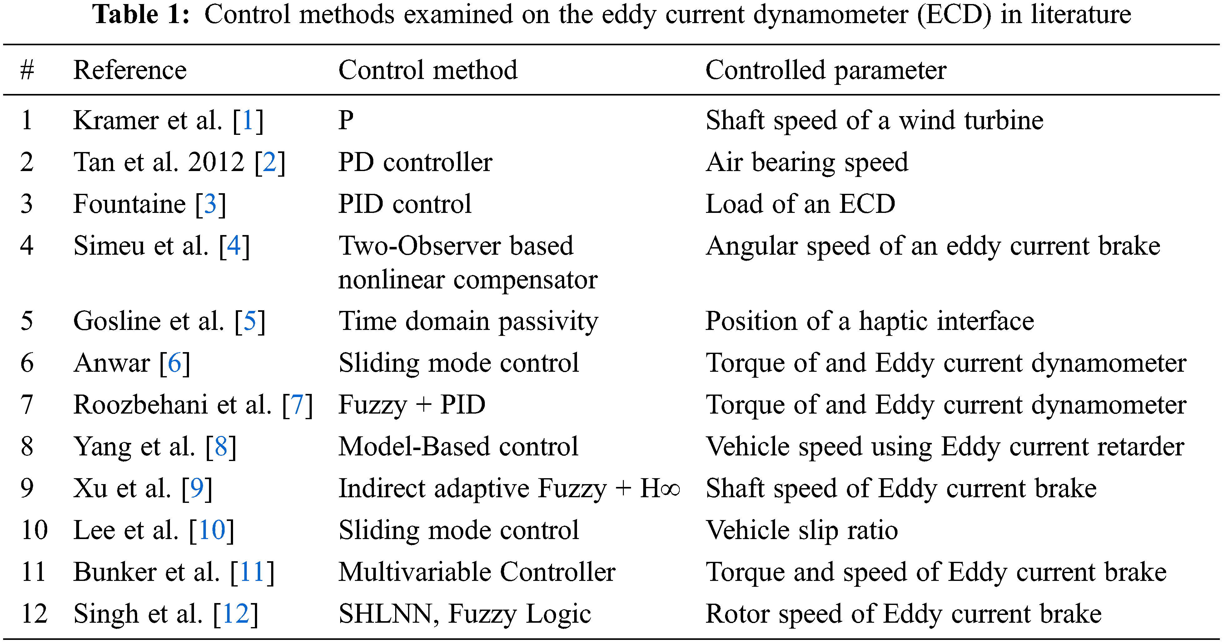
There are many studies focused on controlling the Eddy Current Dynamometers and related brake techniques. Tab. 1 summarizes selected studies presenting the results for the control methods examined on Eddy Current Dynamometers in literature. The Eddy current dynamometers are considered to be highly nonlinear braking systems. It is also observed that the braking performance of the system varies with non-linearity with variation of process parameters. It is noted that main approach for overcoming the problem of control of such systems is based on using non-linear control methods. Each of these methods brings adaptiveness but with disadvantages such as chattering. Since MPC is a linear control approach and only it is only valid for the given mathematical model, it is noted that there is a need for artificial intelligence-based control method of Eddy Current Dynamometers.
The recent studies on Artificial Intelligence with increased computing capability attract attention of researchers to MPC enhanced by AI learning methods. Lin et al. [13] used BP neural network-based online model predictive control strategy to deal with the time variance and nonlinearity of forging process. Overcome nonlinearities and low output accuracy of the transplanting manipulator. Moreover, Zhao et al. [14] designed an ANN (Artificial Neural Network) for MPC for damping DC voltage smaller steady-state error and a dynamic voltage overshoot on aircraft systems. Yan et al. [15] handled the NMP problem by using ANN supervised MPC system. RBNN coupled with MPC was demonstrated to be effective in the paper of Huang et al. [16] for clutch control, Han et al. [17] for optimization of wind turbines, Mirzaeinejad [18] for controlling of wheel slip in antilock braking systems, Jamil et al. [19] for controlling control of vibrations in tall structure. Also, Muhammad et al. [20] carried out ANFIS reinforced MPC algorithm for another nonlinear system of urea plant reactor unit and Pang et al. [21] for Omni-Directional Service Robot.
In the presented work, following novelties are offered;
1. The use of an Artificial Intelligence coupled Model Predictive Controller for Eddy Current Dynamometers.
2. To test and appraise the efficacy of the proposed technique, it is implemented on an Eddy Current Dynamometer.
3. The proposed four Artificial Intelligence techniques are also compared with each other, i.e., GRNN, RBNN, SHLNN and ANFIS. The methods are then tested, validated and compared. To the best of authors’ knowledge, the Artificial Intelligence based Model Predictive Controller has not been implemented and validated for such a large sized Eddy Current Dynamometers in literature.
Numerous Artificial Intelligence-based control studies on other mechanical and other various systems showed us these methods bring robustness and adaption ability for control systems without any drawbacks. Therefore, this study features an adaptive model predictive control method using various artificial intelligence methods to predicting real-time the mathematical model of the system. Hence, this approach allows achievement of a system reaction data to maximize the MPC performance. Finally, the results of the performance comparison for SHLNN, GRNN, RBNN and ANFIS learning performance techniques are presented based on the MAPE statistics technique.
The experiments presented in this study are performed in the Laboratories of Automotive Engineering Department at Cukurova University. A schematic shows the illustration of the test setup dynamometer. Fig. 1 shows the scheme of the dynamometer setup that includes a 3.1-liter internal combustion engine with 71 horsepower maximum power at 2500 rpm used for generation of the motion. The employed Eddy Current Brake has a maximum braking torque of 650 Nm at 1000 rpm angular velocity to load the IC engine.

Figure 1: Schematic of eddy current dynamometer
Fig. 2 illustrates the electronic assembly of the system. Eddy Current Brake power supply has an 80 A PWM output with a resolution of 1023 leading to 0.0782 A resolution. Test rig sensory system consists of a load cell to measure the torque, a line drive encoder with 360 pulses each revolution to shaft speed and an infrared contactless temperature sensor is mounted on stator of eddy current brake to measure the rotor temperature. Humutech MF634 Data Acquisition card is placed on the PC to connect the test rig and control system setup due to its versality and MATLAB/Simulink link ability.
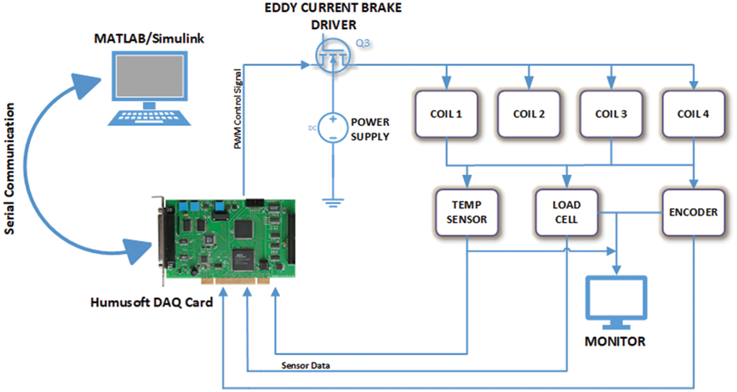
Figure 2: The electronical control schema
The Eddy Current Dynamometer assembly is illustrated in Fig. 3. The dynamometer setup is integrated at a connecting bearing. The connecting bearing joints rotor and stator which the load cell and the coils that conducts magnetic field are assembled to form the system. A connecting shaft is used to join the rotor and internal combustion engine to Eddy Current Brake and its encoder. Typically, the Eddy Current Dynamometers (ECD) are designed to test and validate operating conditions of motor applications, motor control research, production and repair tests. The braking force of ECD varies linear generally between 0–1000 rpm values. On the other hand, at the higher speeds, braking torque acts nonlinearly due to the nature of the magnetic field related iron loss, skin effects, demagnetizing effects and insufficient time for inducing the eddy currents.
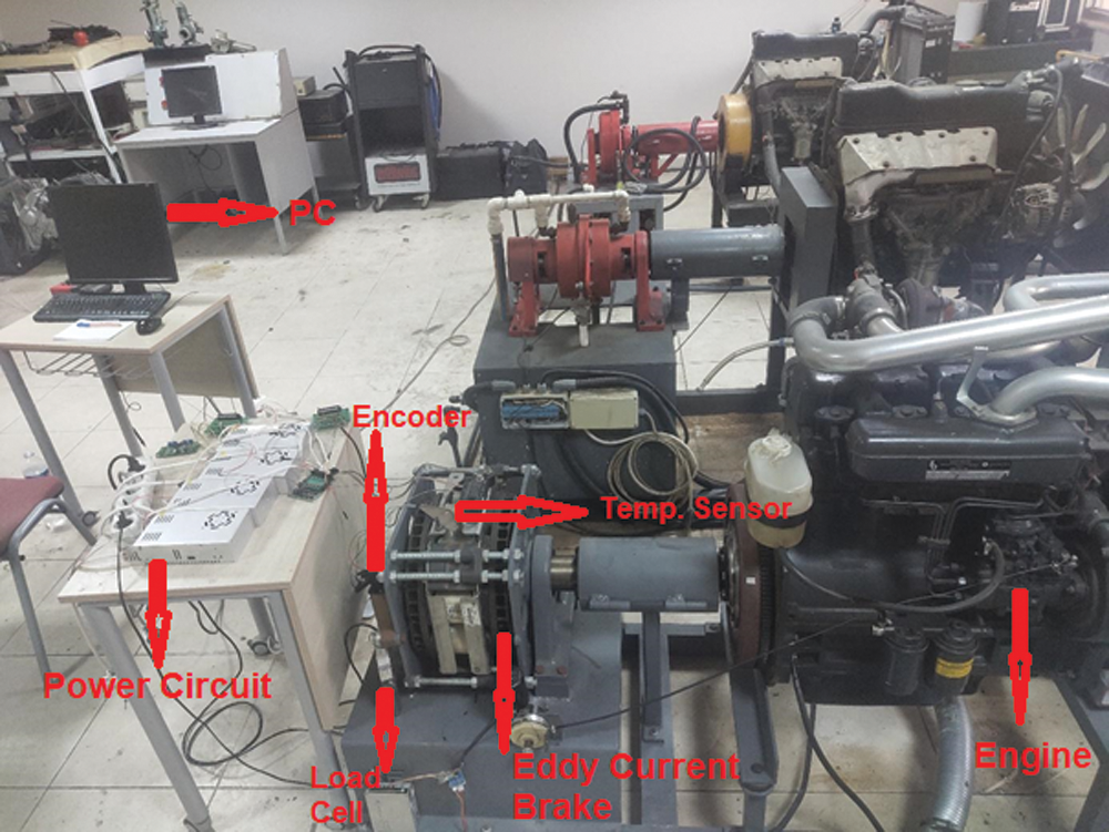
Figure 3: Photo of the eddy current dynamometer
Nature of the ECB is nonlinear with respect to rotor temperature and speed. Hence, system identification and parameter estimation has been performed in order to determine system parameters at each case as 2nd order linear system using MATLAB System Identification Toolbox as seen on Fig. 4. System model and related parameters are shown on Eq. (1).
where Tw (reverse of the natural frequency) is natural period, ζ damping ratio and K is the process gain. The settling time and final torque values of step response graph leads us to calculate Tw an K. Mathematical model of the ECD model structure is selected as underdamped pair which means transfer function with a pair of complex-conjugate poles. MATLAB system identification toolbox is used for estimation of the model parameters by minimizing the error between measured output and estimated model with help of iterative estimation algorithm.
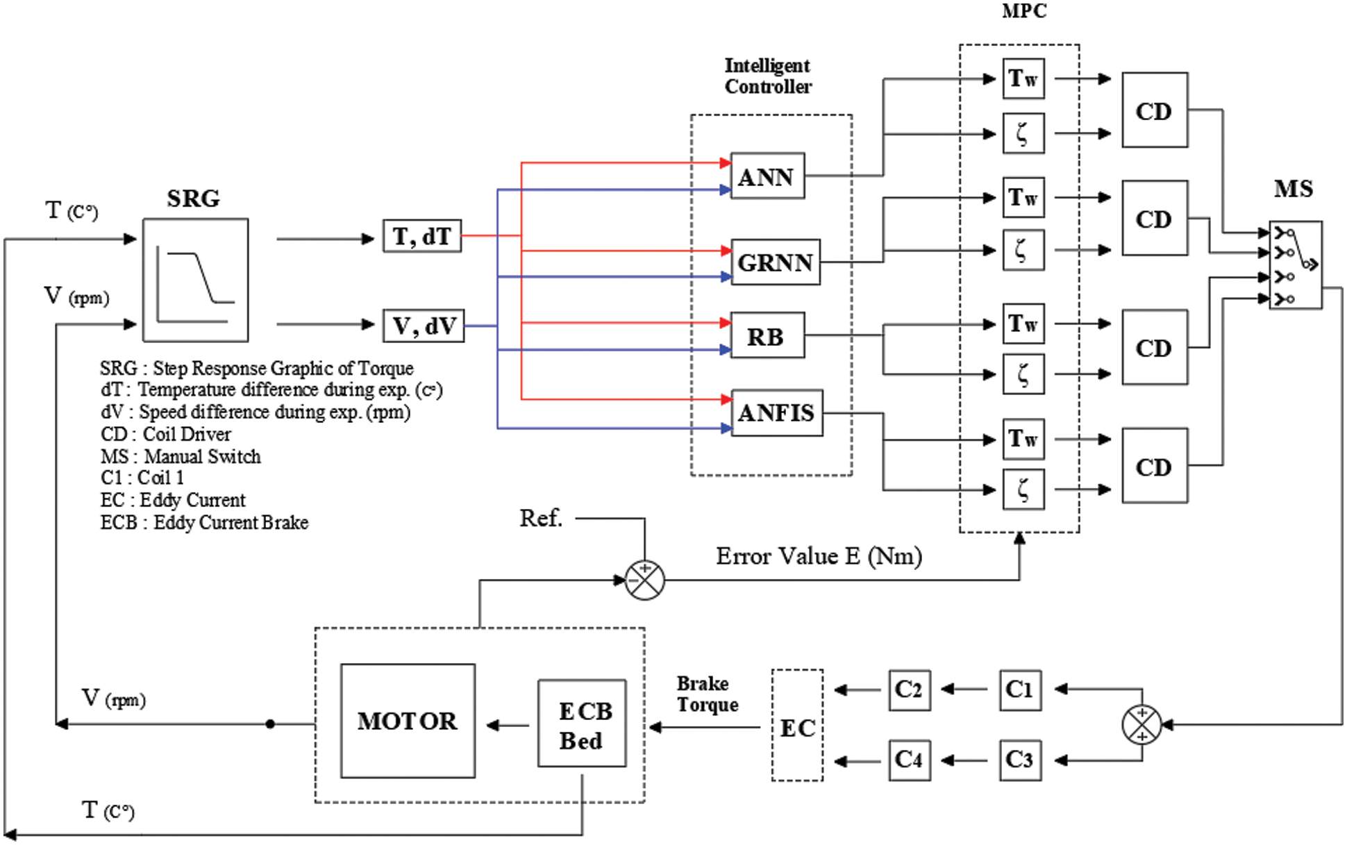
Figure 4: Block diagram of adaptive MPC control
Step response of the Eddy current dynamometer has been investigated at between 1600–3000 rpm with steps of 100 rpm as well as rotor temperature at intervals of 25°C–75°C. The resulting torque values and step input are measured and recorded. Therefore, nonlinear system is linearized at several points and the datasets required for the AI methods are stored. The system starts gathering the 4-input data from sensors and temperature and speed difference from step response curves, and sends the collected information to AI algorithms. These algorithms then update the model of the MPC which calculates the optimum control signal according to models at each time step. The calculated control signal is received by coil driver and then the coil driver deploys the required power to eddy current brake coils which leads desired amount of braking. Finally, an online adaptive control system task is completed. Fig. 4 shows detailed block diagram of designed MPC on ECD.
The MPC technique is defined by Camacho et al. [22] as “Model predictive control refers to the class of control algorithms that compute a manipulated input profile by utilizing a process model to optimize an open loop performance objective subject to constraints over a future time horizon”.
MPC working principle can be seen in Fig. 5. The outputs in the future are predicted at each step of the process, with help of a model that takes the input values and outputs into account. The control horizon is the place where the values are calculated. In Fig. 5, the future (u(n + k) for k = 1…C) and past inputs (u(n - k) for k = 1…M-1) are shown respectively. The set of future inputs that are computed as a function of the past inputs are used to minimize the error. Only u(n + 1) t is applied since new data can only be considered at the next step. This procedure is called receding strategy [23].
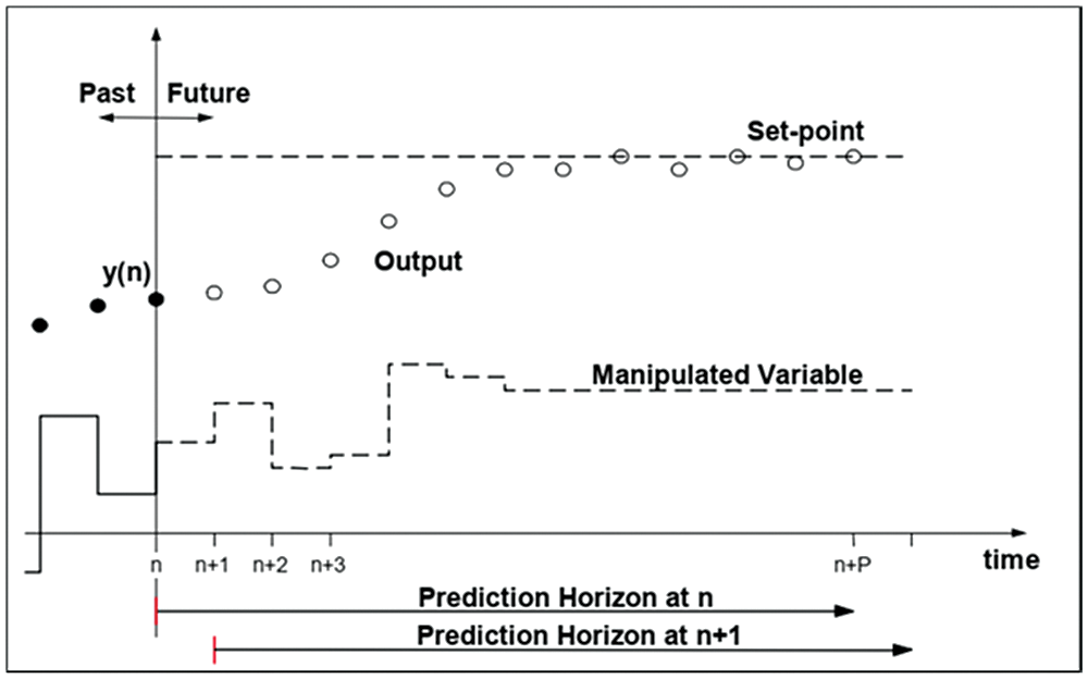
Figure 5: MPC strategy
Fig. 6 shows the basic outline of the MPC. A mathematical model is offered to predict the future outputs evolved from earlier inputs and outputs of the system. The predicted output of the plant and the reference trajectory of output are compared, and calculations are made in order to determine the future errors of the plant at each time step. Best future inputs considering the constraints and objective function are calculated by the MPC optimizer. Only the first element of this optimal set is applied to the plant and the same procedure repeated at the next sampling time. This procedure requires a high amount of computing power.
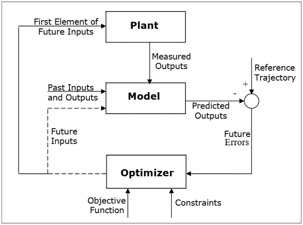
Figure 6: Basic structure of MPC
Model Predictive Control (MPC) has become a mature control strategy over the last few years because it can take in account explicitly different types of constraints on input and output signals. It can handle a large class of systems especially the delayed systems. However, it also increases the computation complexity, especially for the nonlinear system having high orders [24,25].
2.2.2 Single Hidden Layer Hidden Network (SHLNN)
Yavuz et al. [26] states that the biological nervous systems and mathematical systems’ learning theories inspired the Artificial Neural Network (ANN). The learning procedure is achieved by a various mesh of processing nodes and connections. The Neural Networks are simply defined as “massively parallel interconnected networks of simple (usually adaptive) elements and their hierarchical organizations which are intended to interact with objects of the real world in the same way as biological nervous systems do”.
Living neurons have three parts called as dendrites spread out of the cell body, a cell nucleus (processor) and an axon (output) which The ANN imitates biological neural structure via activation functions, adjustable weights, and nodes. The adjustable weights equal to biological synapses. A positive weight symbolizes an excitatory connection. A negative weight symbolizes a blocking connection. The weighted inputs to a neuron are summed up and then proceed to an activation function which states the neuron’s response.
The main parts of single-layer ANNs are input and output nodes. Connections can be varied between different input and output variables (C). The output nodes must be connected with all input nodes.
The Multi-layer networks are forwardly connected and consist of three different layers. These layers are the input layer, hidden-layers, and output layer as seen on Fig. 7. The Multi-layer networks use the supervised learning technique. The learning rule of the multi-layer network is a generalized version of the Delta learning rule. The generalized delta rule consists of two stages. The first stage is the forward calculation and the second stage is backward calculation. Unconditionally, there is an activation function in every neuron structures. This function is usually the sigmoid function. Here, the important thing is the function must be derivable. As in the backward calculation, the derivative of the function used here will be taken. The preferred training algorithm in this study was Levenberg-Marquardt. Two-layer feed-forward network consist of sigmoid hidden neurons and linear output neurons. While training NNs at the MATLAB/Simulink, Neural Fitting (nftool) Toolbox was used. Details of the networks are restricted by the Neural Fitting Toolbox.
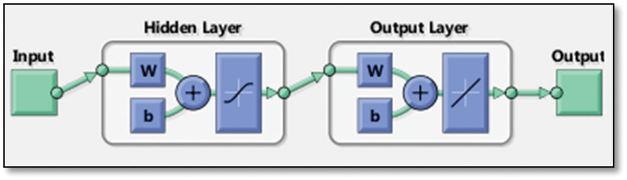
Figure 7: SHLNN structure
There are various kinds of neural networks (NNs) that can be used for various purposes in literature. One example of such is the Generalized Regression Neural Network (GRNN). This specific neural network is commonly used for functions that are approximation-oriented with Gaussian activation function in the hidden layer. A Generalized regression neural network (GRNN) is suitably designed for function approximation purposes. The GRNN achieves higher convergence and faster learning due to its ability to handle the varying number of samples. It also requires less datasets to be considered its advantages. The structure of GRNN is shown in Fig. 8.
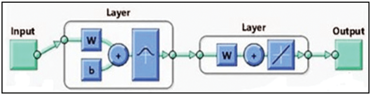
Figure 8: GRNN structure
Radial basis neural networks are ideal for system control applications. They have various advantages such as good design, good tolerance to noise, and an online learning capability. The properties of radial basis neural networks make them very suitable for designing flexible control systems for system control applications and approximation purposes. Details of the structure can be seen in Fig. 9.
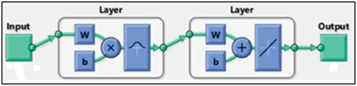
Figure 9: RBNN structure
The ANFIS word comes from adaptive neuro-Fuzzy interference. ANFIS creates a Fuzzy interference system (FIS) using a chosen input/output dataset. FIS membership function parameters are adjusted (tuned) with the help of back-propagation algorithm or hybrid version of least square method and back-propagation algorithm. Hence, the tuning process lets the Fuzzy systems learn from the input/output data block.
FIS is one of the most popular artificial intelligence methods. It is solely based on human expert experience to decide. Therefore, success of FIS decisions is related with either the accuracy of experts or converting these experiences from real world to Fuzzy Logic interface. Unlike FIS, ANFIS does not need expert experience. Instead, ANN techniques using input/output date sets are used. Structure of used ANFIS can be seen on Fig. 10.
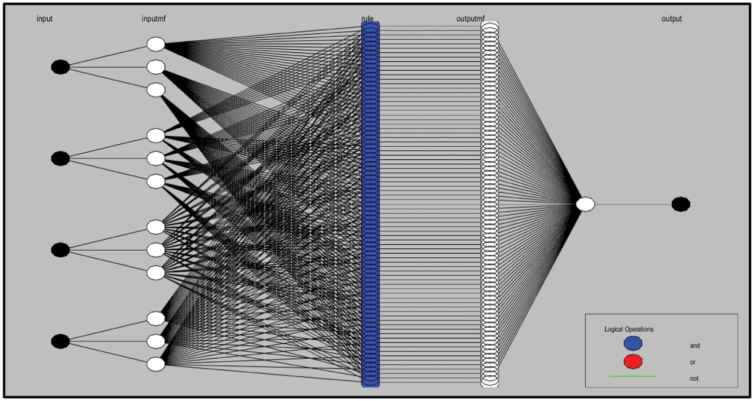
Figure 10: Sample of an ANFIS structure
The main advantages of ANFIS are;
✓ Fuzzy Logic is tolerant of incorrect data.
✓ ANFIS can design nonlinear functions of arbitrary complexity using data blocks.
✓ Can be coupled with various control techniques. In this paper, ANFIS and Model Predictive Control techniques are augmented.
Fig. 11 depicts that there are 4 inputs for the offered artificial intelligence methods. These are gathered from system identification and parameter estimation process. The step response starting speed is first speed and step response finish speed is layered as second speed while starting rotor temperature named as starting temperature and finished rotor temperature as second temperature. The predicted outputs are Tw, K are finally found by SHLNN, GRNN, RBNN and ANFIS.
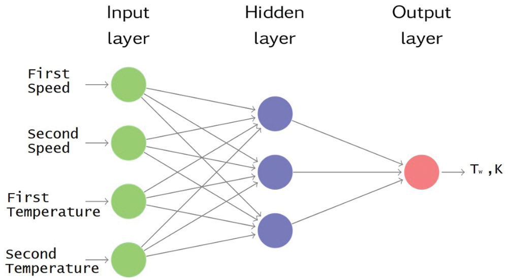
Figure 11: Learning structure for predictions
The convergence of results is performed by the mean average percent error (MAPE) given by Eq. (2):
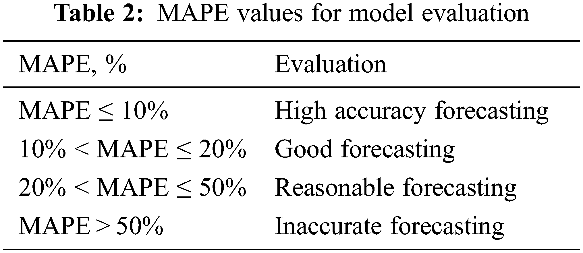
Mean absolute error, root-mean-square error, and MAPE are generally used to measure the accuracy of forecasts. The smaller the values of aforementioned performance parameters, the better forecast accuracy. MAPE criterion is more decisive among others since it is stated in easy equivalent percentage terms. Tab. 2 demonstrates typical MAPE values for model assessment [27].
MPC system is designed to provide optimum control based on mathematical model and manipulated variable. As the temperature and speed of ECD rotor is changed, Artificial intelligence algorithms renew the mathematical model at each time step in real-time. Hence times step should be small enough to catch every important dynamic information. For this purpose, sample time of the MPC is set to 0.1 s. Prediction and control horizon have a huge impact on prediction success of the MPC. Therefore, after several trial-and-error process, prediction and control horizon are found to be 10 and 3.
A Single Hidden Layer Neural Network, a General Regression Neural Network, and a Radial Basis Neural Network and an ANFIS structure are constructed based on system dynamics and previous studies. The gathered experiment results prove that training algorithm of back-propagation is substantially satisfactory for predicting system parameters natural period (Tw), Process Gain (K) and Damping ratio (ζ) for various shaft speeds, Eddy Current Brake rotor temperature values. ζ is not added to training since it is found to be 0.9 for all scenarios. The performance of learning algorithms is tested with a set of experiment data which is not included to training data in order to eliminate memorizing phenomena and find out real performance for SHLNN, GRNN, RBNN and ANFIS. The training dataset for all methods includes 73 lines of data and constant 9 of them were picked as the testing data for each AI structures to avoid calculation error.
2 SHLNN structures are configured separately for Tw and K. Structure for Tw has 100 hidden layers and best validation performance found at epoch 4 while 22nd epoch was the best performance point of structure for K with 10 hidden layers and the training algorithm is Levenberg-Marquardt back propagation (trainlm). 64 rows of input data are presented randomly while 70% (44) of input data is used for training job, 15% (10) is used as validation job, lastly, 15% (10) is used as testing. 9 selected data from outside are used for testing of built SHLNN structure. The comparison of the SHLNN output vs. experiment data can be seen on Fig. 12.
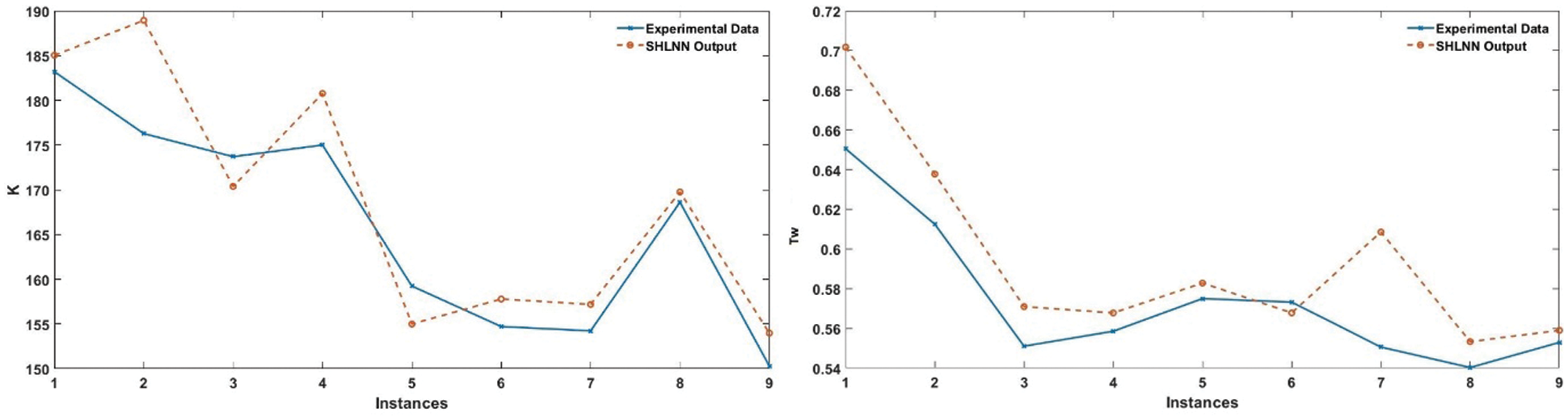
Figure 12: Comparison between experimental data and SHLNN prediction
Spread value has a vital role for GRNN and RBNN algorithms GRNN and RBNN algorithms. 1, 5, 25, 50, 75, 100, 150, 250, 750, 1750, 3000 spread values were tried to optimize the spread number for Tw and K with 64 training data and 9 test data. Customization of spread value is executed using trial and error method. As for the obtained results, using GRNN, MAPE values for Tw and K are 2,4019 and 1,855 at 25 and 5 spreads, respectively. The comparisons can be seen on Fig. 13.
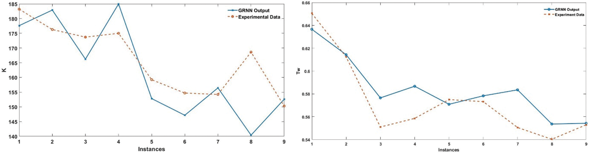
Figure 13: Comparison between experimental data and GRNN prediction
Likewise, 9 randomly selected experimental data which is apart from training dataset is taken into account for testing. MAPE results of RBNN are found as 3,134 for Tw and 3,091 for K at 150 and 25 spreads. The K value for test data varies between 185 to 140 and Tw between 0.55 and 0.66. Thus, Tw values are calculated between 0.7 and 0.56. The details of performance comparison are depicted on Fig. 14.
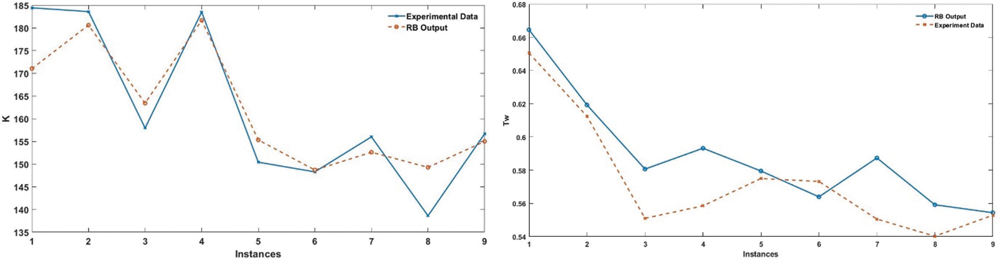
Figure 14: Comparison between experimental data and RBNN prediction
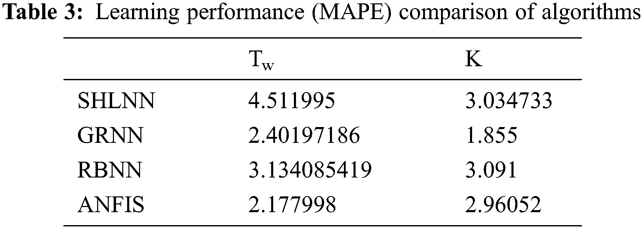
Performance of ANFIS compared to experimental data for Tw and K are given in Fig. 15 and it is shown that results are highly successful with a MAPE number of 2,178 for Tw and 2,9605 for K. Best performances of ANFIS for Tw is achieved with 16 Gaussian type membership function at 640 epochs. ANFIS structure that is designed for K has 12 Gaussian type membership functions reached the best error at 800 epochs. Hybrid optimization method is used for both training. General performance comparison summed up on Tab. 3.
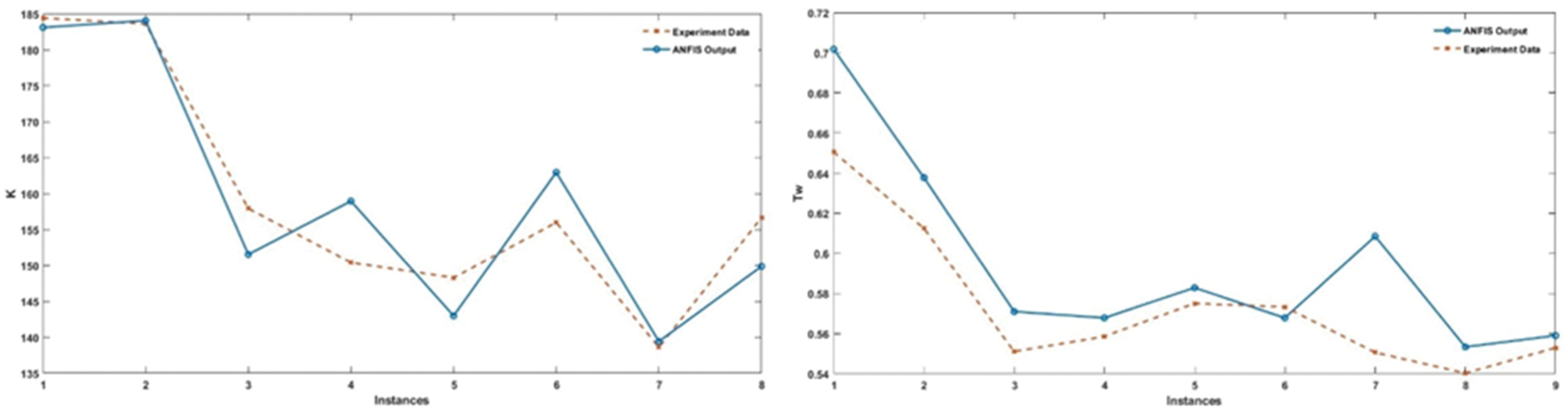
Figure 15: Comparison between experimental data and ANFIS prediction for K
MATLAB/Simulink is used due to its advanced synchronous real-time control and soft computing capability. In our system, data from 2 sensors (line drive encoder and temperature sensor) are fed into Simulink environment by analog and digital input blocks. The Simulink has a control block specialized for adaptive MPC which leads to rearrange model continuously. In addition, prediction and control horizon are also set on its interface. The calculated transfer function by AI blocks is also converted to state-space model by necessary Simulink blocks. Fig. 16 illustrates the responses of MPC coupled with ANFIS, SHLNN, GRNN and RBNN. Reference torque value for the test experiment is 50 N.m. Speed and rotor temperature was chosen apart from the training data. Results show that rise times of all algorithms are almost the same and it is 1.8 s. On the other hand, GRNN has the least overshoot of 0.21 N.m and SHLNN has 0.68 N.m meaning the biggest overshoot. In addition, ANFIS and RBNN has 0.42 N.m and 0.48 N.m overshoot, respectively. Finally, an adaptive MPC control system is successfully adapted. The test experiment proves that offered AI couple MPC controllers are successfully working.
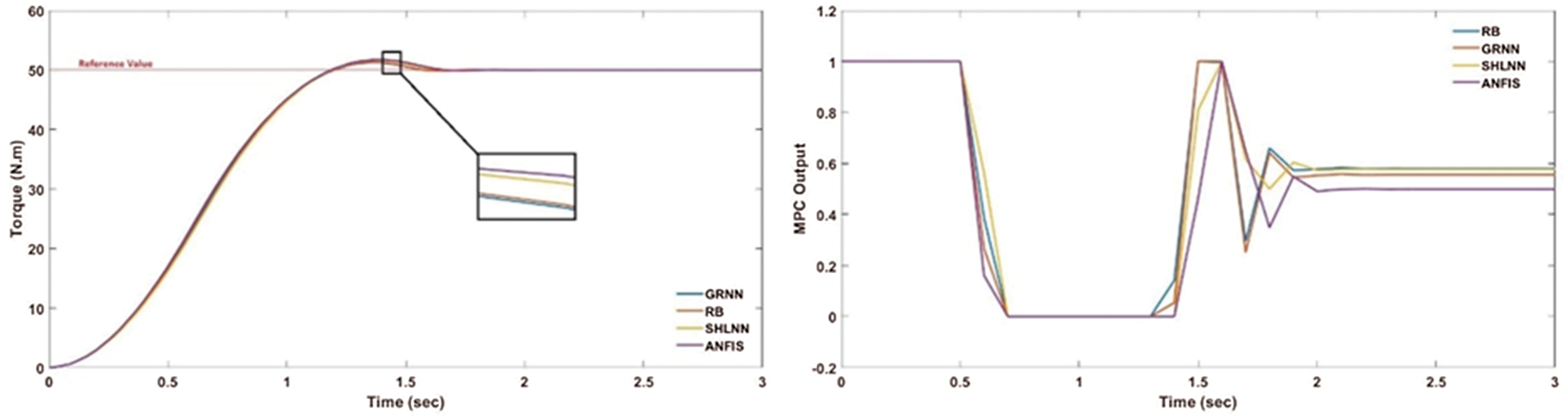
Figure 16: Results of MPC coupled artificial intelligence methods
The Eddy Current Dynamometers are non-contact, electrically powered brakes especially used as auxiliary braking devices and automotive industry testing equipment comes with complications to control due to nonlinearities. In this study, SHLNN coupled MPC, GRNN coupled MPC, RBNN coupled MPC and ANFIS coupled MPC control methods are investigated for the Eddy Current Brake engine test bed. The results show that all control methods show qualified performance while GRNN brings the best performance with MAPE values of 2.4(Tw) and 1.855(K). The SHLNN approach proposes 4.51(Tw) and 3.03(K) values that is being observed to be as the worst in system performance. In addition, ANFIS has a slightly better performance than RBNN. In conclusion, coupling with AI methods increases the capabilities and eliminates the weakness of MPC.
Acknowledgement: I would like to acknowledge TEMSA and BAŞAK Truck Companies for their retarder, and IC engine grants.
Funding Statement: The authors received no specific funding for this study.
Conflicts of Interest: The authors declare that they have no conflicts of interest to report regarding the present study
1. V. Kramer, R. Mishra, P. Brauneis and K. Schmidt, “Utilization of a hardware-in-the-loop-system for controlling the speed of an eddy current brake,” in 25th Int. Congress on Condition Monitoring and Diagnostic Engineering, Huddersfield, UK, pp. 364, 2012. [Google Scholar]
2. K. K. Tan, S. N. Huang, C. S. Teo and R. Yang, “Damping estimation and control of a contactless brake system using an eddy current,” in IEEE ICCA 2010, Xiamen, China, pp. 2224–2228, 2010. [Google Scholar]
3. A. Fountaine, “Design of an engine test cell control system,” Ph.D. dissertation University of Windsor, Canada, 2012. [Google Scholar]
4. E. Simeu and D. Georges, “Modeling and control of an eddy current brake,” Control Engineering Practice, vol. 4, no. 1, pp. 19–26, 1996. [Google Scholar]
5. A. H. Gosline and V. Hayward, “Eddy current brakes for haptic interfaces: Design, identification, and control,” IEEE/ASME Transactions on Mechatronics, vol. 13, no. 6, pp. 669–677, 2008. [Google Scholar]
6. S. Anwar, “A parametric model of an eddy current electric machine for automotive braking applications,” IEEE Transactions on Control Systems Technology, vol. 12, no. 3, pp. 422–427, 2004. [Google Scholar]
7. S. Roozbehani, S. Saki, H. Nazifi and K. Kanzi, “Identification and fuzzy-PI controller design for a novel claw pole eddy current dynamometer in wide speed range,” in 24th Iranian Conf. on Electrical Engineering (ICEE), Shiraz, Iran, pp. 1038–1042, 2016. [Google Scholar]
8. J. Yang, F. Yi and J. Wang, “Model-based adaptive control of eddy current retarder,” in Chinese Control and Decision Conf. (CCDC), Shenyang, China, pp. 1889–1891, 2018. [Google Scholar]
9. X. Xu, T. Zhu, S. Chen and C. Wang, “Design and indirect adaptive fuzzy H∞ control of a novel retarder coupled with eddy current effect and MR effect,” Journal of Intelligent Material Systems and Structures, vol. 13, no. 6, pp. 640–660, 2020. [Google Scholar]
10. K. Lee and K. Park, “Optimal robust control of a contactless brake system using an eddy current,” Mechatronics, vol. 9, no. 6, pp. 615–631, 1999. [Google Scholar]
11. B. J. Bunker, M. A. Franchek and B. E. Thomason, “Robust multivariable control of an engine-dynamometer system,” IEEE Transactions on Control Systems Technology, vol. 5, no. 2, pp. 189–199, 1997. [Google Scholar]
12. A. K. Singh, I. Nasiruddin, A. K. Sharma and A. Saxena, “Modelling, analysis, and control of an eddy current braking system using intelligent controllers,” Journal of Intelligent & Fuzzy Systems, vol. 36, no. 3, pp. 2185–2194, 2019. [Google Scholar]
13. Y. C. Lin, D. D. Chen, M. S. Chen, X. M. Chen and J. Li, “A precise BP neural network-based online model predictive control strategy for die forging hydraulic press machine,” Neural Computing and Applications, vol. 29, no. 9, pp. 585–596, 2018. [Google Scholar]
14. D. Zhao, K. Shen, L. Chen, Z. Wang and W. Liu, “Improved active damping stabilization of dab converter interfaced aircraft dc microgrids using neural network-based model predictive control,” IEEE Transactions on Transportation Electrification, (Early Access), 2021. [Google Scholar]
15. Y. Yan and Q. Xu, “Neural networks-based model predictive control for precision motion tracking of a micro positioning system,” International Journal of Intelligent Robotics and Applications, vol. 4, pp. 164–176, 2020. [Google Scholar]
16. C. Huang, X. Wang, L. Li and X. Chen, “Multistructure radial basis function neural-networks-based extended model predictive control: Application to clutch control,” IEEE/ASME Transactions on Mechatronics, vol. 24, no. 6, pp. 2519–2530, 2019. [Google Scholar]
17. B. Han, X. Kong, Z. Zhang and L. Zhou, “Neural network model predictive control optimisation for large wind turbines,” IET Generation, Transmission & Distribution, vol. 11, no. 14, pp. 3491–3498, 2017. [Google Scholar]
18. H. Mirzaeinejad, “Robust predictive control of wheel slip in antilock braking systems based on radial basis function neural network,” Applied Soft Computing, vol. 70, pp. 318–329, 2018. [Google Scholar]
19. M. Jamil, M. N. Khan, S. J. Rind, Q. Awais and M. Uzair, “Neural network predictive control of vibrations in tall structure: An experimental controlled vision,” Computers & Electrical Engineering, vol. 89, pp. 106940, 2021. [Google Scholar]
20. A. Muhammad, Y. Y. Nazaruddin and P. I. Siregar, “Design of nonlinear adaptive-predictive control system with ANFIS modeling for urea plant reactor unit,” in 6th Int. Conf. on Instrumentation, Control, and Automation (ICA), Bandung, Indonesia, pp. 147–152, 2019. [Google Scholar]
21. F. Pang, M. Luo, X. Xu and Z. Tan, “Path tracking control of an omni-directional service robot based on model predictive control of adaptive neural-fuzzy inference system,” Applied Sciences, vol. 11, no. 2, pp. 838, 2021. [Google Scholar]
22. E. F. Camacho, C. Bordons and J. E. Normey-Rico, Model Predictive Control. Berlin, Germany: Springer, 1999. [Online]. Available: https://link.springer.com/book/10.1007/978-0-85729-398-5. [Google Scholar]
23. I. Aşar, “Model Predictive control (MPC) performance for controlling reaction systems,” Thesis (M.S.M.E.T.U., Turkey, 2004. [Google Scholar]
24. D. Shi, S. Wang, Y. Cai, L. Chen, C. Yuan et al., “Model predictive control for nonlinear energy management of a power split hybrid electric vehicle,” Intelligent Automation and Soft Computing, vol. 26, no. 1, pp. 27–39, 2020. [Google Scholar]
25. A. Rhouma, S. Hafsi and F. Bouani, “Practical application of fractional order controllers to a delay thermal system,” Computer Systems Science and Engineering, vol. 34, no. 5, pp. 305–313, 2019. [Google Scholar]
26. H. Yavuz and S. Beller, “An intelligent serial connected hybrid control method for gantry cranes,” Mechanical Systems and Signal Processing, vol. 146, pp. 107011, 2021. [Google Scholar]
27. S. Yıldırım, E. Tosun, A. Çalık, İ. Uluocak and A. Avşar, “Artificial intelligence techniques for the vibration, noise, and emission characteristics of a hydrogen-enriched diesel engine,” Energy Sources, Part A: Recovery, Utilization, and Environmental Effects, vol. 41, no. 18, pp. 2194–2206, 2019. [Google Scholar]
 | This work is licensed under a Creative Commons Attribution 4.0 International License, which permits unrestricted use, distribution, and reproduction in any medium, provided the original work is properly cited. |