DOI:10.32604/csse.2023.025434
| Computer Systems Science & Engineering DOI:10.32604/csse.2023.025434 | |
| Article |
Weed Classification Using Particle Swarm Optimization and Deep Learning Models
1Department of Computer Science and Engineering, Thiagarajar College of Engineering, Tamil Nadu, India
2Department of Information Technology, Thiagarajar College of Engineering, Tamil Nadu, India
*Corresponding Author: M. Manikandakumar. Email: mmrit@tce.edu
Received: 23 November 2021; Accepted: 10 January 2022
Abstract: Weed is a plant that grows along with nearly all field crops, including rice, wheat, cotton, millets and sugar cane, affecting crop yield and quality. Classification and accurate identification of all types of weeds is a challenging task for farmers in earlier stage of crop growth because of similarity. To address this issue, an efficient weed classification model is proposed with the Deep Convolutional Neural Network (CNN) that implements automatic feature extraction and performs complex feature learning for image classification. Throughout this work, weed images were trained using the proposed CNN model with evolutionary computing approach to classify the weeds based on the two publicly available weed datasets. The Tamil Nadu Agricultural University (TNAU) dataset used as a first dataset that consists of 40 classes of weed images and the other dataset is from Indian Council of Agriculture Research – Directorate of Weed Research (ICAR-DWR) which contains 50 classes of weed images. An effective Particle Swarm Optimization (PSO) technique is applied in the proposed CNN to automatically evolve and improve its classification accuracy. The proposed model was evaluated and compared with pre-trained transfer learning models such as GoogLeNet, AlexNet, Residual neural Network (ResNet) and Visual Geometry Group Network (VGGNet) for weed classification. This work shows that the performance of the PSO assisted proposed CNN model is significantly improved the success rate by 98.58% for TNAU and 97.79% for ICAR-DWR weed datasets.
Keywords: Deep learning; convolutional neural network; weed classification; transfer learning; particle swarm optimization; evolutionary computing
Weeds grow along with the crop, which causes problems in irrigation due to its competition and interference behaviour. They increase the cost of farming requirement and hinder the progress of irrigation work by distressing the operation of farm machinery. This reduces the quality of the crop, slows the cultivation process and reduces farm productivity. In particular, weed species such as Cicuta virosa (cowbane), Torilis japonica (hedge parsley), Datura stramonium (Jimson weed), Sinapis arvensis (wild mustard) and Allium ursinum (wild garlic bulblets) are especially toxic and life-threatening [1]. Few weeds serve as nests for insects and pests. They damage native plants, wildlife and create troublesome eco systems including forests, watersheds and rivers. Specific weeds such as conium maculatum are poisonous to livestock that can affect animal health and yield such as milk and meat. Few aquatic weeds change the appearance of water and its taste [2]. At the same time, weed control using herbicides and pesticides would generate degradation of the soil and reduce the land value. Eradication of most of the environmental weeds is a real challenge that can be achieved by adopting modernization [3,4].
Currently, there are many research projects in the field of weed management. In general, automation of weed control, smart weed management, and smart agriculture are usually some key terms where the Information and Communication Technology (ICT) plays a major role. Weeds can be differentiated from the crop by their spectral reflectance and color characteristics. Misclassification of classes in the classification technique can cause excessive loss in crop yield, generate unintentional harm to the crop, thereby leading to complete removal of crop as well. Identifying the location and density of the weed is the most important task in a wide-range crop, and this can be achieved by a visual method called computer vision. Machine learning approaches and computer vision-based methodologies are developed by researchers to learn the shape, color and texture features of crop and weed classification. Machine vision approaches are a way of detecting the weeds by separating plant pixels from soil using the color variations [5].
Many recent works have shown that CNN models based on deep learning have strong feature learning and state-of-the-art performance on various agricultural issues such as plant disease classification, weed classification, pest identification and fruit classification. Ghazi et al. have evaluated GoogLeNet, AlexNet and VGGNet models using transfer learning to boost the accuracy of identification of plant species [6]. In addition, enhancement in weed classification schemes are highly invited in weed control practices. Current CNNs have made a clear observation that some shortcut connections were proposed to integrate the layers that are not close to one other in several models, such as ResNet [7] and Densely connected Networks (DenseNet) [8]. The classic feed-forward architecture has been upset by these shortcuts, allowing for more flexible CNN structures. Aside from this challenge, the manual design of CNN’s requires in - depth knowledge and takes time because each design attempt must be trained using the Stochastic Gradient Descent (SGD) algorithm, which is sluggish for deep CNNs. As a result, in recent times, there has been a resurgence in research for optimal CNNs. In this field, Evolutionary Computation (EC) could be extensively used to autonomously evolve CNNs with significant performance improvement similar to Reinforcement Learning approaches [9–11].
In this present work, a deep CNN model is proposed with an evolutionary computation technique to classify the weeds of two publicly available datasets. Transfer learning based pre-trained deep CNN models like GoogLeNet, AlexNet, ResNet and VGGNet are implemented for comparison of results. The deep learning models are implemented using Python framework with Keras libraries 2.3.1, Tensorflow 2.2.0 as a backend [12] and performed on NVIDIA GTX 1650 GPU processors for parallelization and for faster training. The purpose of this research is to classify weed images with improved performance using an efficient PSO assisted deep CNN model and to further experiment with pre-trained CNN models using transfer learning to investigate the essential hyper parameters to avoid over-fitting and classification errors. PSO will be employed as the optimization algorithm because it is very simple EC algorithm that is both computationally economical and successful for optimizing a wide variety of functions [13].
Remaining part of the paper is organized as follows: Section 2 explains the materials and methodology used in the proposed work. Section 3 depicts various transfer learning models for weed classification, analysis of different hyperparameters of proposed CNN model represented in Section 4, and Section 5 summarizes and discusses the results. Section 6 eventually concludes the work with further improvements.
In this work, the weed dataset is collected from TNAU with 40 weed classes (http://agritech.tnau.ac.in/agriculture/agri_weedmgt_fieldcrops.html) and from ICAR-DWR with 50 weed classes (http://weedid.dwr.org.in/). Although the weed images are collected from Indian databases, they commonly exist in most of the countries. According to the global distribution details from Global Biodiversity Information Facility (GBIF), all the weed classes used in this research are more widespread throughout the world. Before using the images directly into the deep learning models, the Red, Green, Blue (RGB) images of both datasets are pre-processed using image pre-processing techniques to extract weed from the original input image [14,15]. Initially, the edge detection and noise suppression tasks are performed by Canny Edge Detector algorithm. An outline of the images is defined by (x, y, w, h) coordinates where (x, y) is the rectangle’s top-left point and (w, h) is its width and height. Each outline of the image is calculated and all the weed images are resized to 224 × 224. Fig. 1(i) shows pre-processed input image of the TNAU weed dataset before being cropped and Fig. 1(ii) shows the cropped image as mentioned. Region of Interest (RoI) of the weed is extracted whenever the width and height are greater than 100 pixels.
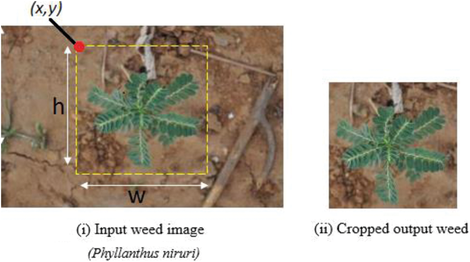
Figure 1: Pre-processed weed image (TNAU dataset)
The image augmentation mechanisms like scaling, random rotation, transposing, horizontal and vertical flip – shift are applied to increase the weed image count of the datasets. These pre-processing mechanisms enhanced the efficiency of the weed classification operation considerably. Tab. 1 summarizes the number of images in training and testing sets, the weed samples for 40 classes of TNAU dataset illustrated in Fig. 2., and the samples of ICAR-DWR dataset are given in Fig. 3.
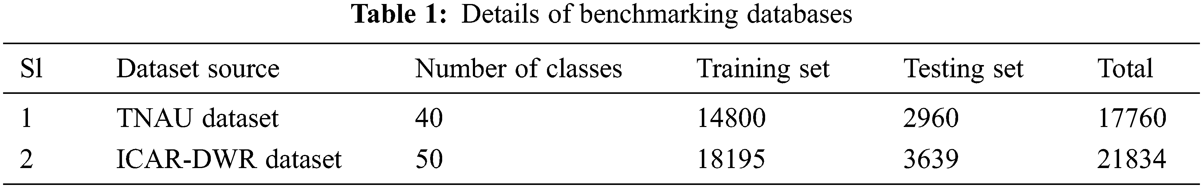
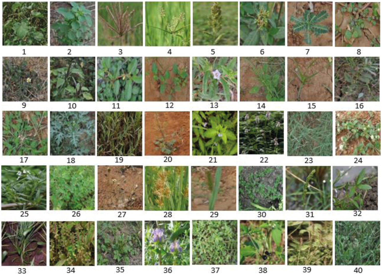
Figure 2: Samples of weed classes in TNAU dataset
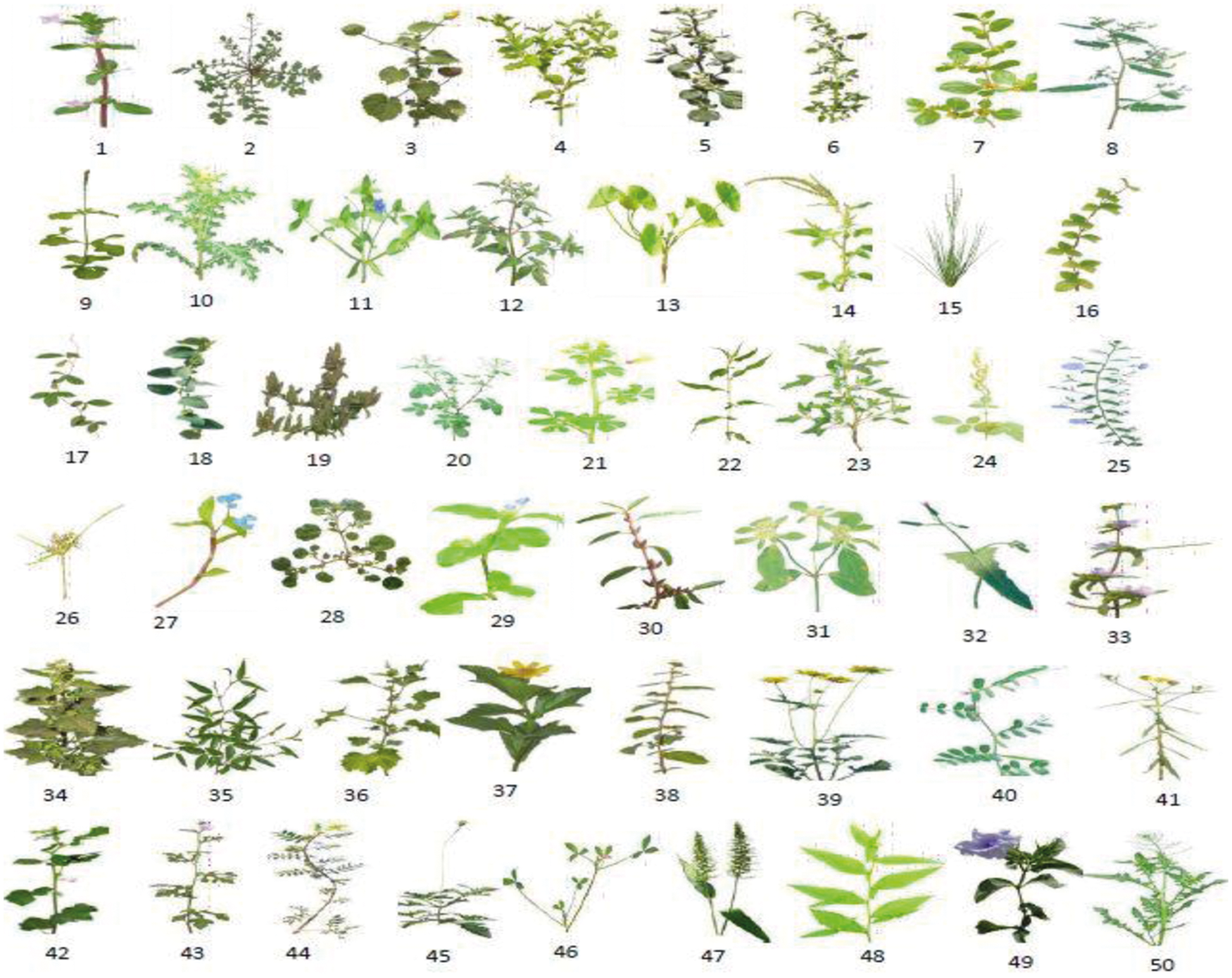
Figure 3: Samples of weed classes in ICAR-DWR dataset
In this proposed work, the experiments were conducted on TNAU and ICAR-DWR weed datasets separately. To establish the classification, each weed dataset is split into two groups i.e., training and testing dataset. The training dataset contains 80% of the weed images of each class and the testing dataset contains 20% of the remaining weed images of each class.
2.2 Proposed CNN Weed Classification Model
CNN is one of the emerging neural networks that use deep learning to perform cognitive, generative and descriptive operations such as object detection, image classification, image recognition etc., Building any kind of CNN involves major operations such as Convolution, Pooling, Flattening and Full connection (FC). i.e., In order to train and test in a deep CNN model, each input image will pass through a series of convolution layers with filters, flattening followed by pooling layers and fully connected layers. The aim of this work is to identify the class of input image. Keras is one of the popular deep learning libraries, which is used here to build the CNN [16].
The testing process is done in this research by using Tensorflow as a backend and sequential network is used to initialize the CNN model. Weed images are basically in two-dimensional arrays and sized as 224 × 224, where Conv2D is imported to perform the convolution operation. At this convolution operation, Conv2D function creates an initial convolution kernel of 5 × 5 sizes that will convolve with the input to generate output. Initially, the function uses 32 filters which decide the dimensionality of the output space. The feature map is generated by the convolution for each filter [17–19]. The function takes input as RGB color images with 64 × 64 resolutions and for activations, the model makes use of the rectifier function ReLU (Rectified Linear Unit). ReLu computes the function as defined in Eq. (1).
where, parameter x is the input tensor and slope of the negative part considered as zero and max() returns maximum value for the output. This ReLu activation function returns the value as per the Eq. (2).
where, α is a small constant value.
2.2.3 Feature Learning and Pooling
Pooling operation is performed after the convolution using MaxPooling2D function to build CNN. The reason for selecting MaxPooling2D is that it will generate the maximum value pixel from the respective RoI. This operation decreases the image size as much as possible resulting in a decrease in the total number of nodes for the upcoming layers. Here MaxPooling2D specifies the pooling window 2 × 2. It will halve the input in both vertical and horizontal dimensions to minimize loss of pixels and get a precise region.
2.2.4 Flattening and Connection
The flattening process converts the resulting two-dimensional arrays into a single long linear vector. To build the fully connected neural network, dense layers have been imported to connect the set of nodes. These nodes will work as input nodes to fully-connected layers. One of the parameters in the dense function is the units which refer to the number of nodes present in this hidden layer and the rectifier activation function is another important parameter. The Softmax function sets the calculated probability values for each class. The full connection layer connects all output features of the final convolutional layer. Fig. 4 Illustrates the proposed CNN classification process with the sample input image and the corresponding classified label (highlighted).
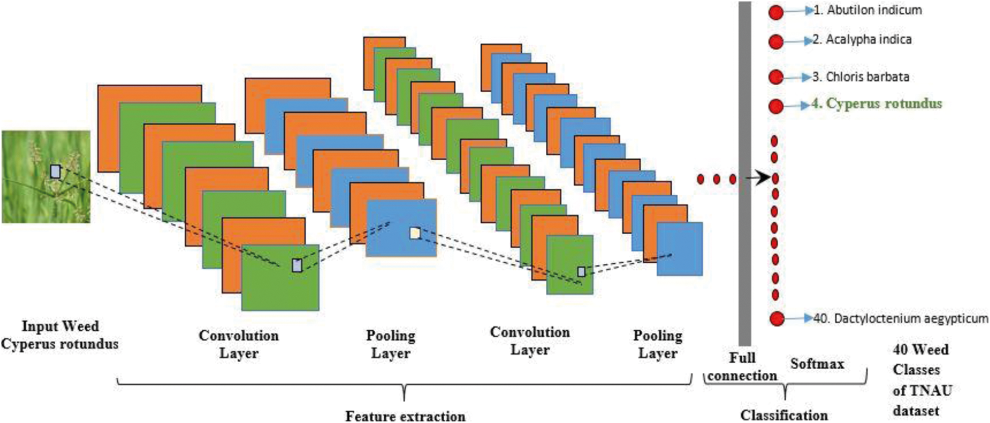
Figure 4: Proposed CNN architecture for weed classification
2.2.5 Weed Classification Architecture
The proposed CNN elements essentially measure the linear combination of RGB images, and apply the softmax activation function to the fully connected layer to produce the neural network nonlinearity. Eq. (3) defines the softmax function.
where, θ is one-hot encoded matrix and x is the trained set of features.
On building the final CNN, the optimizer chooses adaptive moment estimation (Adam) algorithm to minimize the error loss. With 0.99 momentum, the learning rates are defined as 0.0001, 0.001 and 0.01 to reduce the loss function of the proposed network and the loss function used here is, multi-class categorical cross entropy. The number of epochs is varied up to 100 and the mini-batch size is defined as 8, 16, 32, 64, 128 and 150.
In multi-class classification, the cross-entropy can be calculated as per the Eq. (4).
where,
N refers the number of weed samples,
K indicates total number of weed classes,
tij is the ith weed sample belongs to jth weed class,
yij refers the output of the weed sample i for the weed class j
The metrics parameter needed to be chosen to evolve the performance metric. Prior to fitting the image to the proposed CNN, preprocessing was done to prevent the over-fitting [19]. Over-fitting is a challenge that provides good training accuracy and poor testing accuracy for nodes from one layer to another. The proposed model is now being trained on the weed training dataset and the accuracy of weed testing set is estimated. In a specific interval with the validation frequency of 25, the accuracy of the classification shall be calculated as Eq. (5).
2.3 Particle Swarm Optimization
PSO is a bio-inspired, distributed random number system used to search for an optimal solution in the solution space by initializing the population and assigns a random velocity to each particle. It does so by using primitive mathematical operators known as update equations as given in (6)–(8). Vectors are used to denote the particle’s position and velocity.
where, p stands for particles, xi(t) refers the position of particle i at iteration t, r1 and r2 are the random values between 0 and 1. The constants w, c1, and c2 are the input parameters for the PSO algorithm, position pbesti yields the best f(X) value and gbest is investigated by all the particles in the swarm. The present state of the position or velocity is denoted by (t), whereas the future state is denoted by (t + 1).
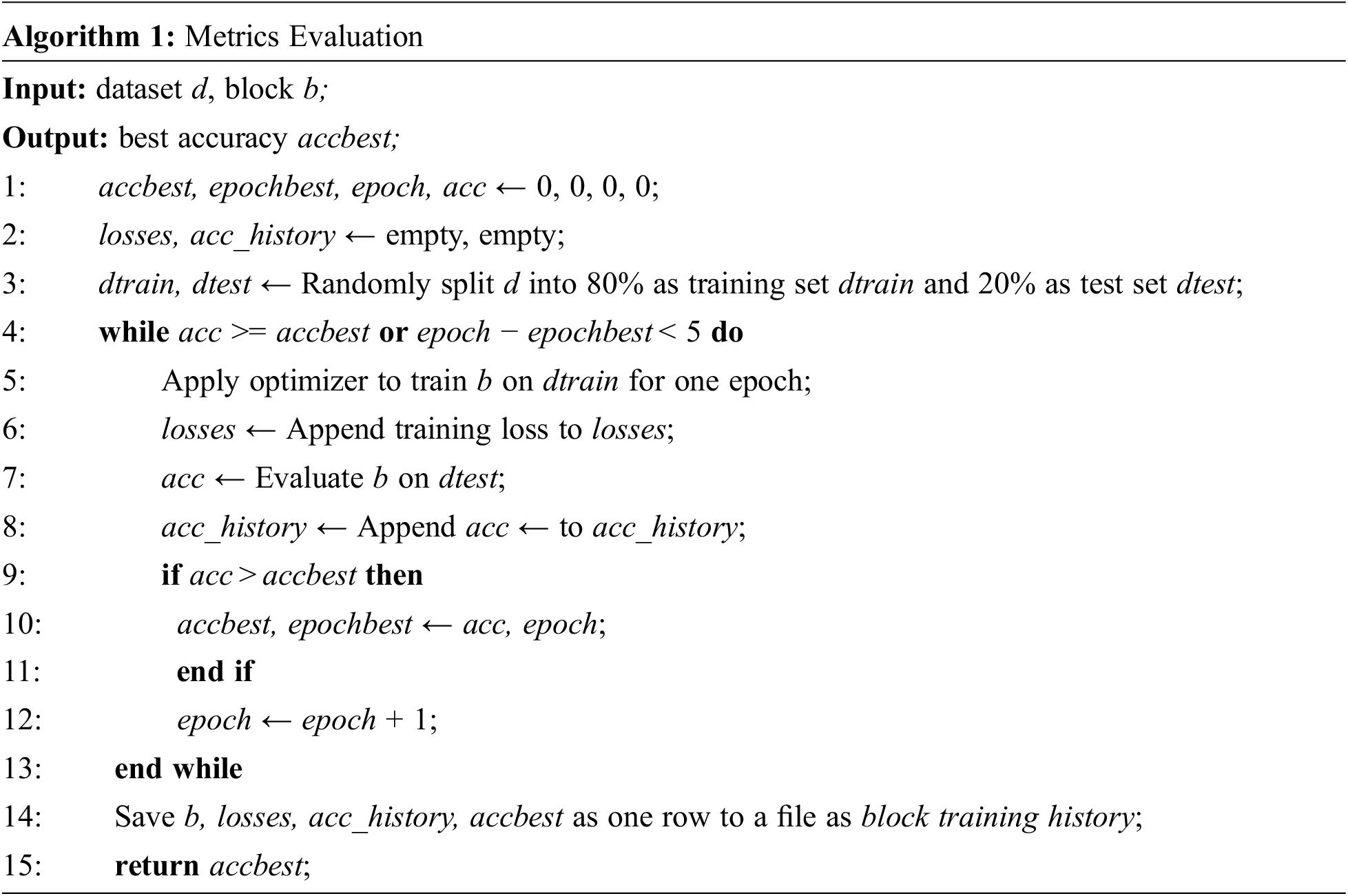
The fitness evaluation methodology is represented in Algorithm 1. The dense block is passed to the evaluation function along with the data set. The training set is used to train the effectiveness of the dense block with SGD. The test set is utilized to evaluate the correctness of the training to produce the classification accuracy, which is used as the fitness value. The results of the training are recorded along with the appropriate classification accuracy. These data are combined and saved as a row in a training history file, which will be used to train the proposed model later. Adam is an optimization algorithm that can improve the training of dense blocks using SGD training method. The learning rate is adjusted according to the training status of the model at specific epoch and hence, Adam gives efficient convergence to accelerate the fitness evaluation.
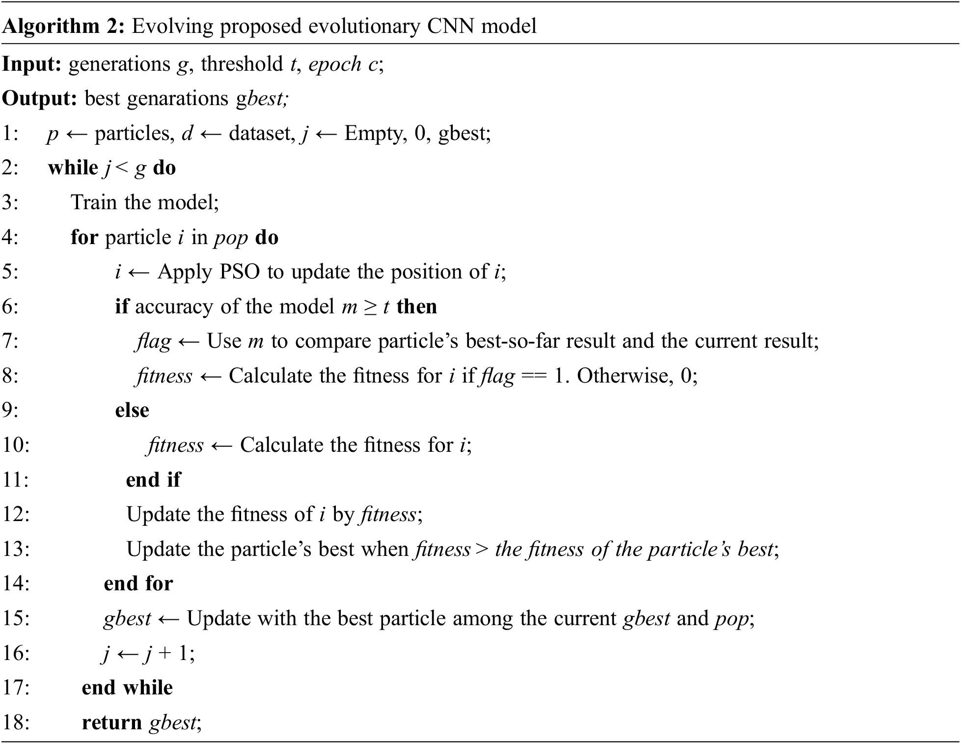
Algorithm 2 depicts the description of the evolutionary process. Using PSO operations, the proposed model converts the variable-length parameters of transferable blocks into a fixed-length vector. Threshold and feature cutting epochs are the two hyperparameters to control the activation of the proposed model. The threshold value can be determined using the mean value of the scores recorded in the training history file during the metrics evaluation phase. The number of epochs utilised to retrieve the losses and accuracies from the block training history is known as the feature-cutting epoch. It is found by determining the smallest cutting point in the training process where learning of entire training process will suffice. To reduce the computational cost, the proposed approach avoids needless metrics evaluation of transferable blocks with poor performance.
Deep CNN based transfer learning approaches such as GoogLeNet, AlexNet, ResNet and VGGNet are applied to retrain the pre-trained deep learning models. Through this transfer learning process, the accuracy and efficiency of the weed classification activities are evaluated with better performance and less computational time. The layered architecture of the model learns the multifaceted features of weed images and is fitted with a fully connected layer to generate the output. The chosen deep leaning models, trained with the TNAU and ICAR-DWR weed datasets are discussed in the subsections.
GoogLeNet or Inception model is a popular deep CNN model that has won ILSVRC2014 competition and achieved the best classification accuracy with top-5 error rate of 6.67% using transfer learning [5,16]. The architecture consists of 2 deep convolution layers (Conv), 4 max pooling layers, 9 linearly stacked inception modules, 1 average pooling layer along with Stride (S), Padding (P), and number of class (C) values as shown in Fig. 5 Each inception module uses 1 × 1 convolutions to do the dimension reduction before moving to larger 3 × 3 and 5 × 5 convolutions. The accuracy of the classification is indicated by the percentage of weed images that the model correctly predicts which is calculated on testing set.
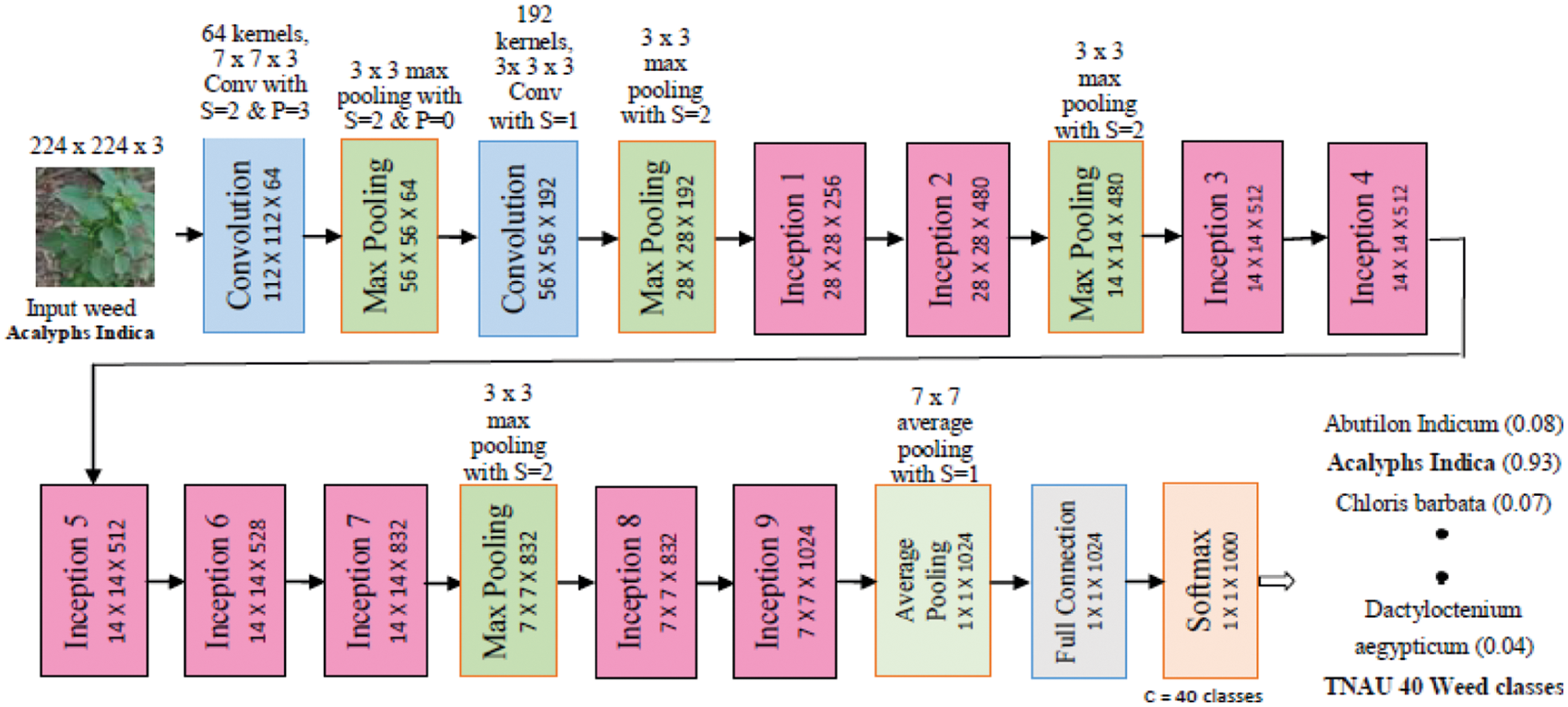
Figure 5: Transfer learning based weed classification using GoogLeNet architecture
The AlexNet input layer is given an input weed image of size 224 × 224 with 3 color planes of TNAU weed dataset. AlexNet consisting of 5 convolution layers, 3 max pooling layers, 3 full connection layers and ReLU is added between every convolution and fully connected layers to increase the non-linearity of the network [18]. The input image is convolved with 96 different 1st layer filters each of the sizes 11 × 11 using a 4 stride in both x and y. Output feature maps are then: (i.) passed through ReLU, (ii.) maxpooling with 3 × 3 regions using stride 2 and (iii.) normalization across feature maps to give 96 different 55 × 55 element feature maps. Same task is repeated in layers 2, 3, 4 and 5. Cross channel normalization is applied before the max pooling layers 1 and 2. The network is actually a larger model and has many parameters, so to minimize over-fitting and training time, dropout regularization with the ratio of 0.5 is applied to first and second fully connected layers. Final layer is the C-way softmax function.
The last three layers of pre-trained AlexNet model is fine-tuned by replacing them with fully connected layer, softmax layer, and an output layer for the weed classification task. The fine-tuned fully connected layer is set to 40 and 50 classes of weeds for TNAU and ICAR-DWR datasets respectively. Accordingly the model is trained with weed image dataset by setting the learning rate, number of epochs, mini-batch size and validation items. To quicken the learning operation, bias learn rate and weight learn rate factors are increased in fully connected layer. The AlexNet network model based on transfer learning is shown in Fig. 6.
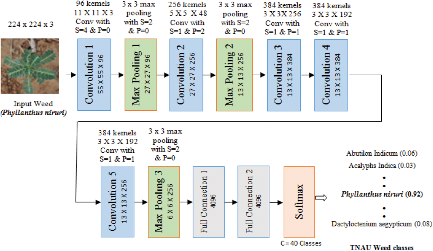
Figure 6: Transfer learning based weed classification using AlexNet architecture
Deep ResNet architecture proves good performance by creating a direct path for spreading information throughout the network. ResNet has skip connections parallel to the normal convolution layers that help the network to learn global features. The skip connection is connected to add the input x to the output after the weight layers. This skip connection enables the model to skip the layers that are not useful and leads optimal tuning for quick training. ResNet allows the blocks for parameterization relative to an identity function and the output H(x) is defined in Eq. (9).
where, F(x) refers the non-linear weight layers.
Two types of residual networks are evaluated for weed classification: ResNet – 50 and ResNet 101. The first two layers of ResNet-50 are same as GoogLeNet which has 7 × 7 convolution layer with 64 kernels, two strides followed by 3 × 3 max pooling layers with a stride of 2. ResNet – 50 has 16 residual building blocks and ResNet – 101 consists 33 residual blocks as seen in Fig. 7. Batch normalization layer is added after each convolution layer in ResNet. The output layer is set to 40, represents the number of weed classes of TNAU dataset.
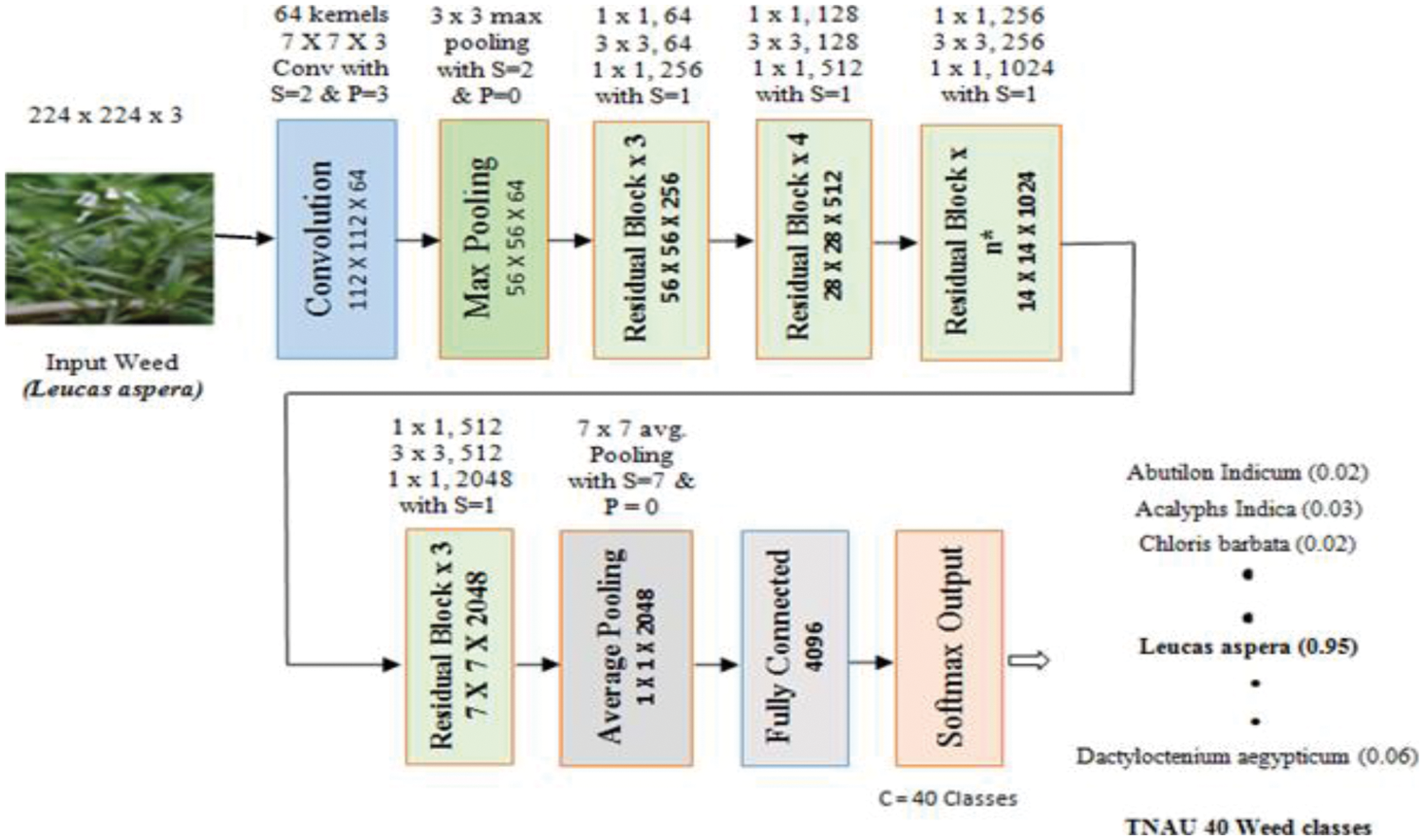
Figure 7: ResNet-50 and ResNet-101 architecture using transfer learning (n* is set to 6 for ResNet-50 and 23 for ResNet-101)
VGGNet was introduced with VGG – 16 and VGG – 19 to improve the training time and to reduce the number of parameters in convolution layers by using 3 × 3 convolution filters [18]. The VGG −16 structure is shown in Fig. 8.
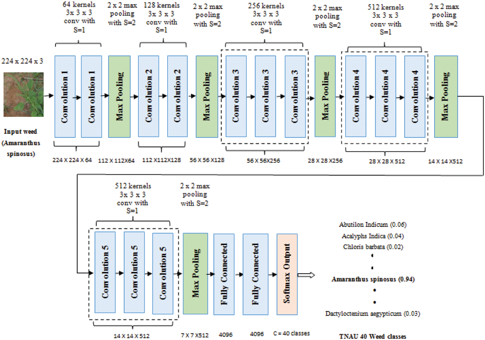
Figure 8: Weed classification using transfer learning with VGGNet model
VGGNet consists of consecutive 3 × 3 convolution layers, 2 × 2 max pooling layers with stride of two, two fully connected layers and finally a softmax output layer. Both VGG-16 and VGG19 variants of VGGNet are used here for the weed image classification which differs only in the total number of layers. The working of VGG – 19 is similar to VGG – 16 model with four 3 × 3 convolution layers in convolution blocks 3, 4 and 5 which is marked by black color dotted blocks in Fig. 8.
4.1 CNN Hyperparameters in Training and Testing
Important hyperparameters such as number of epochs, momentum, learning rate, mini-batch size are applied with specific values in the proposed CNN and the performance metrics are analyzed in the following section.
4.1.1 Effects of Epochs and Momentum
A single unit of epoch is tantamount to doing one-step training on the entire network model. All training samples passes through the deep learning algorithm simultaneously in one epoch before the weights are updated. The training process should always be more than one epoch, increasing the number of epochs would increase the accuracy rate. While fitting the data set to the CNN model, the number of epochs is set as 100 for both the TNAU and ICAR – DWR datasets. But after 30 epochs, the accuracy remains invariable for both the datasets as seen in Fig. 9. The maximum accuracy of 98.58% for the TNAU weed dataset and 97.79% of accuracy for ICAR-DWR weed dataset was achieved due to deep layered structure of the proposed architecture, which gives better weed classification.
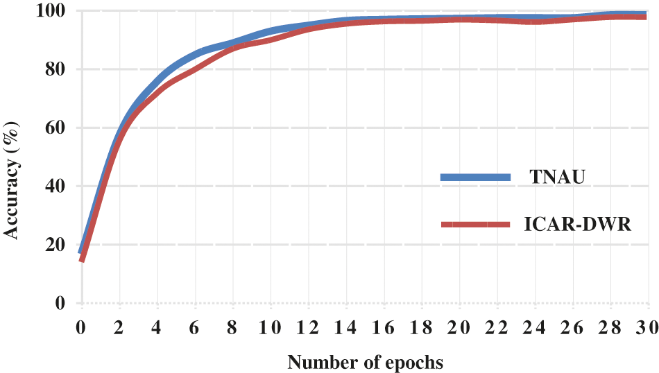
Figure 9: Accuracy rate with number of epochs
Defining the right momentum in the proposed CNN architecture to train the dataset will smooth the learning progress and accelerate training process. Taking into account the number of epochs, the momentum values are evaluated between 0.8 and 0.99 to optimize the training and testing processes. The momentum value 0.99 provided the best results over 0.8 and 0.9; however, the momentum as 0.99 takes more iteration as compared to other values.
4.1.2 Effects of Learning Rate and Batch Size
In training the proposed CNN, the optimal learning rate must be chosen to reduce the loss function in classification of weed. The learning process can be fast due to higher learning rate but increases the loss function. Setting the small learning rate slowly reduces the loss function and prevents the issue of over-fitting. The proposed model is investigated with 0.0001, 0.001 and 0.01 as learning rates and mini-batch size as 64. Based on the classification accuracy as shown in Fig. 10. (i), the better results were achieved while the learning rate was 0.001.
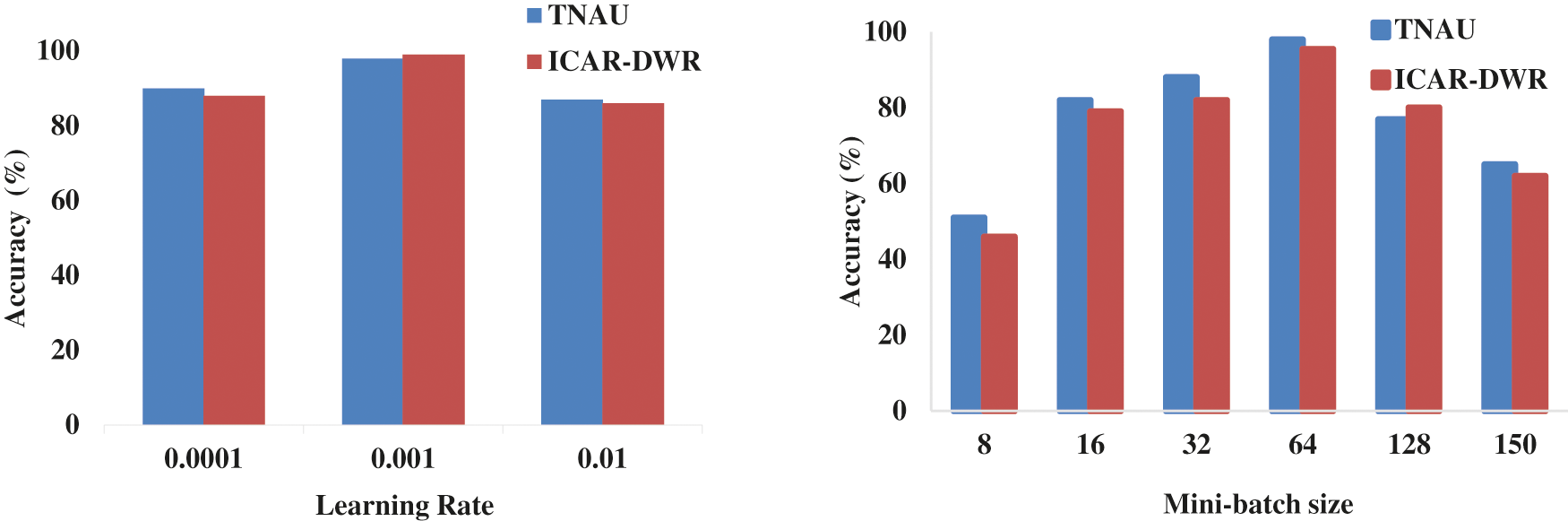
Figure 10: Classification accuracy for different learning rates (i) and mini-batch sizes (ii)
Mini-batch is an important parameter that determines how many samples the model propagates. The model trains the dataset faster and improves the quality with the correct mini-batch size which requires much less memory over larger batch size. For 30 epochs the proposed CNN model is experimented with a batch size of 8, 16, 32, 64, 128 and 150 with the learning rate of 0.001. The efficiency of the model is increased by increasing the batch size from 8 to 64 but it decreased for the batch sizes 128 and 150. As a result, the mini-size batch size of 64 has been set to train the entire model. Fig. 10. (ii) contrasts model performance for TNAU dataset and ICAR-DWR dataset with different mini-batch size.
The performance of the proposed CNN model can be validated by other transfer learning models such as AlexNet, GoogLeNet, ResNet and VGGNet. The specifications of the best hyperparameters as described in Section 3.1 are as follows: Number of epochs – 30, momentum value – 0.99, learning rate – 0.001 and the mini – batch size is 64. Pre-trained transfer learning models perform the feature learning task as much more quickly as possible to perform a classification on weed datasets. Fully connected layers multiply the input matrix with weight matrix in these fine-tuned models, and apply the bias vector. And the weight and bias learn rate factor values of the fully connected layer are increased to accomplish the learning quickly at the new final layers. The PSO parameters are set as follows: inertia weight (w) is 0.729, acceleration coefficient c1 and c2 are 1.496, velocity range is from −10.5 to 10.5, population and generation sizes are 30 and 50 respectively. The transfer learning models were tested using the same hyperparmaeters that were applied to the CNN model being proposed. Fig. 11 shows the overall classification performance of the pre-trained transfer learning models and the proposed CNN model on two weed datasets.
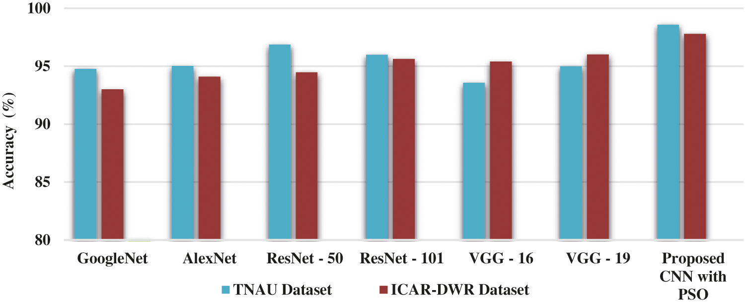
Figure 11: Overall classification accuracies
Among the pre-trained transfer learning models, it can be clearly seen that ResNet – 50 delivers high performance for TNAU (96.88%) and VGGNet −19 performs well for ICAR-DWR (96.02%) weed datasets. ResNet – 50 and ResNet −100 work well with both the weed datasets and are superior to GoogLeNet and AlexNet. From the experiments, the results show that the proposed CNN model has the higher accuracy rate of 98.58% for TNAU weed dataset and 97.79% for ICAR-DWR dataset after performing the hyperparameter tuning and batch normalization processes with six convolution layers. The proposed CNN includes the batch normalization layer between each convolution and the ReLU layers to reduce the over-fitting and improve training performance.
The presence of weeds in the farm is one of the main factors affecting the crop quality and yield. Important goal of this work is to develop the most suitable ways to guarantee a healthy environment and the least impact of troubling weeds. In this work, a deep CNN model is proposed and built to classify the weed. To compare the performance of the proposed CNN model with GoogLeNet, AlexNet, ResNet-50, ResNet-101, VGG-16, and VGG-19, the transfer learning model is implemented. Model hyperparameters such as learning rate, epochs, momentum, mini-batch size have been examined. The proposed CNN uses an effective PSO algorithm to evolve and optimize its classification performance. CNN’s classification accuracy is up to 98.58% for the TNAU dataset and 97.79% for the ICAR-DWR dataset when weeds are classified over 100 different runs. The proposed research is beneficial to farmers in identifying and classifying weeds in the farmland and assists them in taking the required measures to improve crop quality and yield. This approach could be strengthened in the future with more weed classes along with the validation dataset, and combined with an autonomous vehicle’s vision control system to automatically track and eliminate weeds.
Funding Statement: The authors received no specific funding for this study.
Conflicts of Interest: The authors declare that they have no conflicts of interest to report regarding the present study.
1. J. L. Tang, X. Q. Chen, R. H. Miao and D. Wang, “Weed detection using image processing under different illumination for site-specific areas spraying,” Computers and Electronics in Agriculture, vol. 122, pp. 103–111, 2016. [Google Scholar]
2. A. Bakhshipour and A. Jafari, “Evaluation of support vector machine and artificial neural networks in weed detection using shape features,” Computers and Electronics in Agriculture, vol. 145, pp. 153–160, 2018. [Google Scholar]
3. W. Strothmann, A. Ruckelshausen, J. Hertzberg, C. Scholz and F. Langsenkamp, “Plant classification with in-field-labeling for crop/weed discrimination using spectral features and 3D surface features from a multi-wavelength laser line profile system,” Computers and Electronics in Agriculture, vol. 134, pp. 79–93, 2017. [Google Scholar]
4. B. Liu and R. Bruch, “Weed detection for selective spraying: A review,” Current Robotics Reports, vol. 1, no. 1, pp. 19–26, 2020. [Google Scholar]
5. A. Kamilaris and F. X. Prenafeta-Boldú, “Deep learning in agriculture: A survey,” Computers and Electronics in Agriculture, vol. 147, pp. 70–90, 2018. [Google Scholar]
6. M. Mehdipour Ghazi, B. Yanikoglu and E. Aptoula, “Plant identification using deep neural networks via optimization of transfer learning parameters,” Neurocomputing, vol. 235, pp. 228–235, 2017. [Google Scholar]
7. K. He, X. Zhang, S. Ren and J. Sun, “Deep residual learning for image recognition,” in Proc. IEEE CVPR, Las Vegas, NV, USA, pp. 770–778, 2016. [Google Scholar]
8. G. Huang, Z. Liu, L. Van Der Maaten and K. Q. Weinberger, “Densely connected convolutional networks,” in Proc. IEEE CVPR, Honolulu, HI, USA, pp. 2261–2269, 2017. [Google Scholar]
9. M. Dyrmann, H. Karstoft and H. S. Midtiby, “Plant species classification using deep convolutional neural network,” Biosystems Engineering, vol. 151, pp. 72–80, 2016. [Google Scholar]
10. E. Real, A. Aggarwal, Y. Huang and Q. V. Le, “Regularized evolution for image classifier architecture search,” in Proc. AAAI Conf. on Artificial Intelligence, Hawaii, USA, pp. 4780–4789, 2019. [Google Scholar]
11. B. Wang, B. Xue and M. Zhang, “Particle swarm optimisation for evolving deep neural networks for image classification by evolving and stacking transferable blocks,” in Proc. IEEE Congress on Evolutionary Computation (CEC), Glasgow, UK, pp. 1–8, 2020. [Google Scholar]
12. B. Espejo-Garcia, N. Mylonas, L. Athanasakos, S. Fountas and I. Vasilakoglou, “Towards weeds identification assistance through transfer learning,” Computers and Electronics in Agriculture, vol. 171, pp. 105306, 2020. [Google Scholar]
13. Y. Shi and R. Eberhart, “A modified particle swarm optimizer,” in Proc. IEEE Int. Conf. on Evolutionary Computation Proc., Anchorage, AK, USA, pp. 69–73, 1998. [Google Scholar]
14. A. Farooq, J. Hu and X. Jia, “Analysis of spectral bands and spatial resolutions for weed classification via deep convolutional neural network,” IEEE Geoscience and Remote Sensing Letters, vol. 16, no. 2, pp. 183–187, 2019. [Google Scholar]
15. M. Fawakherji, A. Youssef, D. Bloisi, A. Pretto and D. Nardi, “Crop and weeds classification for precision agriculture using context-independent pixel-wise segmentation,” in Proc. Third IEEE Intl. Conf. on Robotic Computing (IRC), Naples, Italy, pp. 146–152, 2019. [Google Scholar]
16. S. H. Lee, C. S. Chan, S. J. Mayo and P. Remagnino, “How deep learning extracts and learns leaf features for plant classification,” Pattern Recognition, vol. 71, pp. 1–13, 2017. [Google Scholar]
17. S. Veeragandham and H. Santhi, “A detailed review on challenges and imperatives of various CNN algorithms in weed detection,” in Proc. Int. Conf. on Artificial Intelligence and Smart Systems, Coimbatore, India, pp. 1068–1073, 2021. [Google Scholar]
18. A. S. M. M. Hasan, F. Sohel, D. Diepeveen, H. Laga and M. G. K. Jones, “A survey of deep learning techniques for weed detection from images,” Computers and Electronics in Agriculture, vol. 184, pp. 106067, 2021. [Google Scholar]
19. A. Milioto, P. Lottes and C. Stachniss, “Real-time semantic segmentation of crop and weed for precision agriculture robots leveraging background knowledge in CNNs,” in Proc. IEEE ICRA, Brisbane, QLD, Australia, pp. 2229–2235, 2018. [Google Scholar]
 | This work is licensed under a Creative Commons Attribution 4.0 International License, which permits unrestricted use, distribution, and reproduction in any medium, provided the original work is properly cited. |