Computer Systems Science & Engineering DOI:10.32604/csse.2023.022047
Article

Designing Bayesian Two-Sided Group Chain Sampling Plan for Gamma Prior Distribution

Waqar Hafeez1 and Nazrina Aziz1,2,*

1School of Quantitative of Sciences, Universiti Utara Malaysia, Sintok, 06010, Malaysia
2Institute of Strategic Industrial Decision Modelling (ISIDM), Universiti Utara Malaysia, Sintok, 06010, Malaysia
*Corresponding Author: Nazrina Aziz. Email: nazrina@uum.edu.my
Received: 26 July 2021; Accepted: 27 August 2021

Abstract: Acceptance sampling is used to decide either the whole lot will be accepted or rejected, based on inspection of randomly sampled items from the same lot. As an alternative to traditional sampling plans, it is possible to use Bayesian approaches using previous knowledge on process variation. This study presents a Bayesian two-sided group chain sampling plan (BTSGChSP) by using various combinations of design parameters. In BTSGChSP, inspection is based on preceding as well as succeeding lots. Poisson function is used to derive the probability of lot acceptance based on defective and non-defective products. Gamma distribution is considered as a suitable prior for Poisson distribution. Four quality regions are found, namely: (i) quality decision region (QDR), (ii) probabilistic quality region (PQR), (iii) limiting quality region (LQR) and (iv) indifference quality region (IQR). Producer’s risk and consumer’s risk are considered to estimate the quality regions, where acceptable quality level (AQL) is associated with producer’s risk and limiting quality level (LQL) is associated with consumer’s risk. Moreover, AQL and LQL are used in the selection of design parameters for BTSGChSP. The values based on all possible combinations of design parameters for BTSGChSP are presented and inflection points’ values are found. The finding exposes that BTSGChSP is a better substitute for the existing plan for industrial practitioners.

Keywords: Bayesian acceptance sampling; poisson distribution; gamma distribution; producer’s risk; consumer’s risk

1  Introduction

Acceptance sampling is a process of testing and deciding to accept or reject the lot as a quality standard. The main purpose of the acceptance sampling is to distinguish between good and poor lots. We have two methods one is 100 percent inspection and the other is sampling inspection. Sampling is more realistic, quicker and cheaper than 100 percent inspection. In sampling inspection, a lot is accepted or rejected based on the number of defective items in the random sample from the lot [1]. Unless the number of defective items exceeds the maximum quantity allowed, the lot is approved.

Bayesian sampling schemes require the user to specifically define the distribution from lot to lot of defects. The prior distribution of the sampling plan is the expected distribution of product quality [2]. The mixture of the prior distribution and evidential skill based on the sample information to the decisiveness of the lot.

Epstein [3], suggested a single sampling plan (SSP) based on the exponential distribution of a submitted lot as a lifetime distribution. Dodge [4] introduced the chain-sampling plan based on SSP by considering multiple samples. It is assumed that the cost is linear in p, which is a fraction of defectives. Hald [5] provided a process for the attribute single sampling plan obtained by minimizing the average cost. Using a gamma prior, Latha et al. [6] addressed a Bayesian chain sampling plan for construction and performance measures.

Mughal et al. [7]; assessed the design parameters for the group acceptance sampling plan (GASP). GASP is evaluated in groups form by using several numbers of testers at a time. Mughal et al. [8] developed an economic reliability GASP by using a group sampling plan for the Pareto 2nd kind distribution. They used Poisson for the biased data theory in finding the necessary design parameters and weighted Poisson distributions. The proposed designs were found to require a minimum testing time.

Mughal et al. [9] developed a GChSP for a product lifetime following the Pareto distribution of the 2nd kind. To satisfy pre-assumed design parameters at several quality stages, lot acceptance probability was obtained. Mughal [10] expanded on and introduced a traditional two-sided group chain sampling plan (TSGChSP) based on [9]. Through considering multiple values of the defective proportion, the minimum sample size and the probability of lot acceptance were found to satisfy the pre-specified consumer’s risk.

Hafeez et al. [11] proposed a Bayesian group chain sampling plan (BGChSP) by considering only preceding lots. They considered binomial distribution and estimate the average probability of acceptance for average proportion of defective. Later, the plan was extended for an average number of defectives by using Poisson distribution and gamma distribution as a prior distribution [12].

Based on [9] and [12] plans, this study concerns the development of a Bayesian two-sided group chain sampling plan (BTSGChSP) that considers preceding as well as succeeding lots. Poisson distribution function is used to estimate the probability of lot acceptance based on conforming and non-conforming products and gamma distribution is used as a suitable prior for Poisson distribution. Also, the plan indexed parameters for acceptable quality level (AQL) and limiting quality level (LQL) are designed. Four quality regions are found, namely: (i) quality decision region (QDR), (ii) probabilistic quality region (PQR), (iii) limiting quality region (LQR) and (iv) indifference quality region (IQR) for the specified values of the number of testers (r), shape parameter (s), preceding i and succeeding j lots. Also, numerical illustrations are provided for the parameters of prior distribution.

2  Methodology

2.1 Operating Procedure

The operating procedure for TSGChSP is based on the following steps:

1.    Select an ideal number of g groups for each lot and assign r items to each group which is the sample size (n = g * r) required.

2.    Count the total number of defectives Nd that are d in current lot, di in preceding i lots and dj in succeeding j lots.

3.    Accept the lot if no defective is found in total Nd = 0, from the current sample, immediately preceding i and succeeding j samples.

4.    Reject the lot if more than one defective is found in the current lot immediately preceding i and succeeding j samples (Nd > 1).

5.    If no defective is found in current sample (d = 0) and the preceding i and succeeding j samples have only one defective in total (di + dj = 1), accept the lot; that means  Nd=1 .

All the above steps can be summarized in a flow chart presented in Fig. 1.

Figure 1: Operating procedure for TSGChSP

For TSGChSP, the above procedure can also be shown through a tree diagram for i = j = 1 in Fig. 2, where D denotes the defective and D¯ denotes non-defective products.

Figure 2: Tree diagram for the proposed sampling plan

From the tree diagram in Fig. 2, it is clear that TSGChSP contains three acceptance criteria (AC). The possible outcomes which comply with the acceptance criteria of chain sampling are {DD¯D¯,D¯D¯D,D¯D¯D¯} . To estimate the probability of acceptance the outcomes can be written in the form of probabilities.

L(p)=P1P0P0+P0P0P1+P0P0P0; (1)

L(p)=2P1(P0)2+(P0)3. (2)

For TSGChSP, the general expression of the probability of acceptance for i = j = 1 from Eq. (3) is:

L(p)=(i+j)P1(P0)i+j+(P0)i+j+1. (3)

When developing the procedures, L(p) can be calculated for the chain acceptance sampling plans, with the assumption that the underlying distribution for the plan is following either binomial or Poisson distribution [1,11–15]. For the average number of defectives, this paper considers Poisson distribution, such that:

p(c)=μcc!e−μ. (4)

For group chain sampling, replace mean μ = np and n = r * g in Poisson probability distribution function (PDF) and solve for c = 0 and c = 1. After solving the probability of lot acceptance for zero and one defective product from Eq. (4), we obtain:

P0=e−(r∗g)p; (5)

P1=(r∗g)pe−(r∗g)p. (6)

After replacing Eqs. (5) and (6) in Eq. (3), we get:

L(p)=e−rgp(i+j+1)+(i+j)rgpe−rgp(i+j+1). (7)

For the equal number of preceding and succeeding lots i = j, Eq. (7) can be written as:

L(p)=e−rgp(2i+1)+2irgpe−rgp(2i+1). (8)

Let us consider gamma distribution as a suitable prior for the Poisson distribution, with PDF:

f(p)=tsΓ(s)ps−1e−tp, (9)

where the shape parameter s > 0, shape and the rate parameter t > 0 with mean μ=st under the proposed sampling plan. For the average probability of lot acceptance, the general expression used in Bayesian [12] is:

P=∫0∞⁡L(p)f(p)dp. (10)

After replacing Eqs. (8) and (9) in Eq. (10) and then from simplification, we get:

P=tsΓ(s)[Γ(s)(rg(2i+1)+t)s+2irgΓ(s+1)(rg(2i+1)+t)s+1]; (11)

P=(trg(2i+1)+t)s+2irgsts(rg(2i+1)+t)s+1. (12)

Upon Replace mean μ=st that gives t=sμ in Eq. (12) and simplifying:

P=(srgμ(2i+1)+s)s+2irgμ(srgμ(2i+1)+s)s+1. (13)

Now simplifying Eq. (13), for s = 1, 2, 3, we get:

P=1rgμ(2i+1)+1+2irgμ1(rgμ(2i+1)+1)2; (14)

P=4(rgμ(2i+1)+2)2+irgμ16(rgμ(2i+1)+2)3; (15)

P=27(rgμ(2i+1)+3)3+irgμ162(rgμ(2i+1)+3)4. (16)

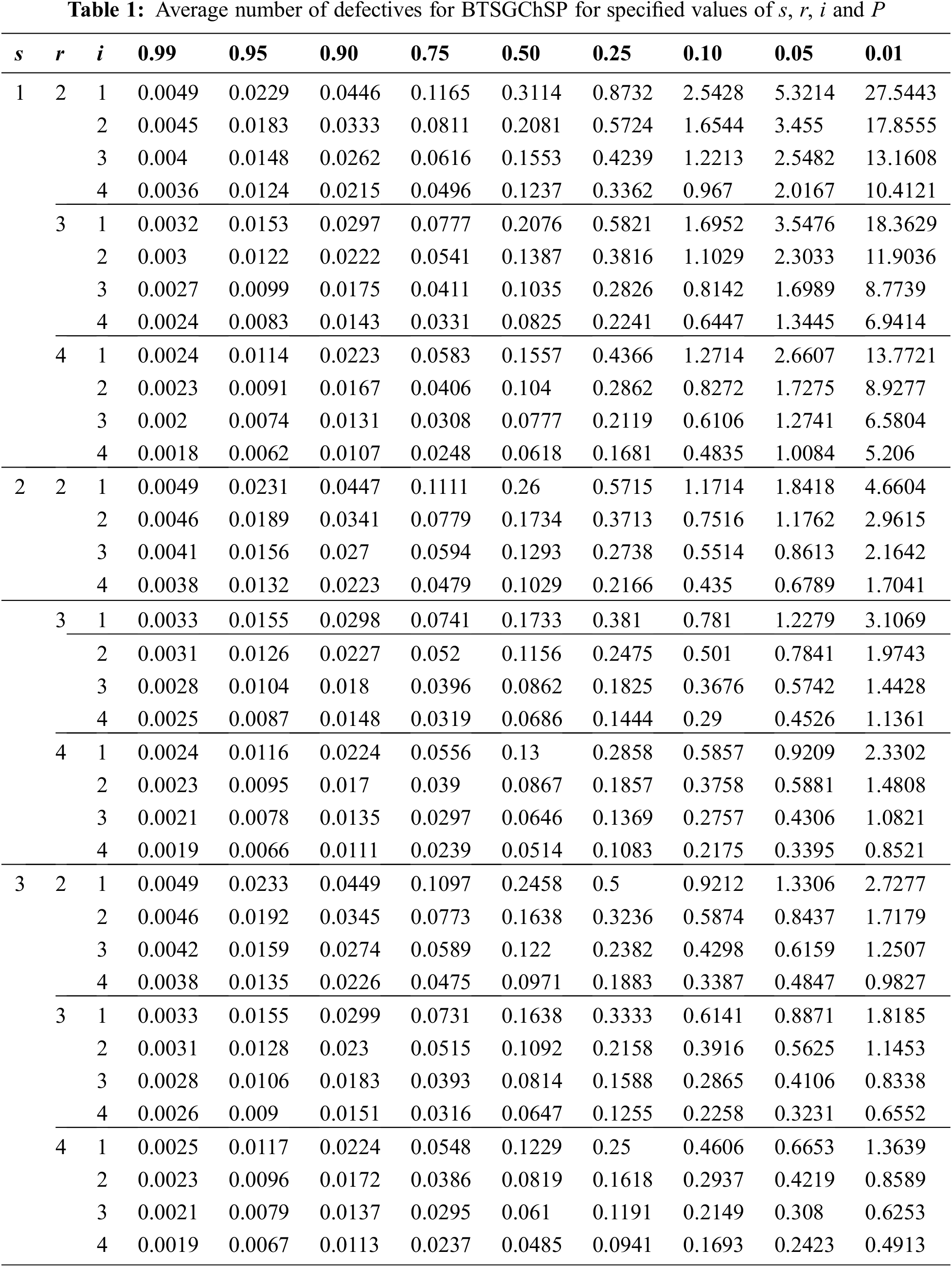
To estimate the quality regions for BTSGChSP, Newton’s approximation is used in Eqs. (14)–(16), where μ is used as a point of control by reducing P. Tab. 1 represents the average number of defectives, for the specified values of shape parameter s = 1, 2, 3; the number of testers r = 2, 3, 4 and number of preceding and succeeding lots i = 1, 2, 3, 4.

2.2 Construction of Quality Regions

2.2.1 Quality Decision Region (QDR)

In this quality region, the product is accepted with the specified quality average by the engineer. Quality is reliably maintained up to μ∗ LQL and a sudden decline in quality are expected. It is defined as (μ1<μ<μ∗) and denoted by d1=μ∗−μ1 derived from the equation of average probability of acceptance, as given in Eq. (13).

P(μ1<μ<μ∗)=(srgμ(2i+1)+s)s+2irgμ(srgμ(2i+1)+s)s+1 (17)

Therefore, gamma is prior distribution with the mean μ=st be the approximate average quality of the product.

2.2.2 Probabilistic Quality Region (PQR)

In PQR the product is accepted with a minimum probability of 0.10 and a maximum probability of 0.95. PQR is defined as (μ1 < μ < μ2) and its range is denoted by d2 = μ2 − μ1 derived from the equation of average probability of acceptance.

2.2.3 Limiting Quality Region (LQR)

The product is accepted with a minimum and maximum probability of 0.1 and 0.9. LQR is defined as an interval like (μ∗<μ<μ2) and denoted by d3=μ2−μ∗ . It is derived from the equation of the average probability of acceptance.

2.2.4 Indifference Quality Region (IQR)

In this quality region, the product is accepted with a minimum probability 0.50 and a maximum of 0.9. IQR is described as (μ1 < μ < μ0) and the range is denoted by d0 = μ0 − μ1. It is derived from the equation of the average probability of acceptance.

2.3 Selection of Sampling Plans

In Tab. 2, the ranges of QDR (gd1), PQR (gd2), LQR (gd3) and IQR (gd0), are shown with corresponding design parameters s, r and i. The defined operating ratios T=μ∗−μ1μ2−μ1=gμ∗−gμ1gμ2−gμ1 , T1=μ∗−μ1μ2−μ∗ and T2=μ∗−μ1μ0−μ1 , are used to characterize the sampling plan. For any given values of QDR (d1), PQR (d2), LQR (d3) and IQR (d0), we can find the operating ratios T=d1d2 , T1=d1d3 and T2=d1d0 . Find the value corresponding to the design parameters s, r and i which is equal to or just less than the specified ratio under the column of T, T1 and T2 in Tab. 2. From this ratio, we can determine the minimum number of groups g and other design parameters for the BTSGChSP.

3  Numerical Examples

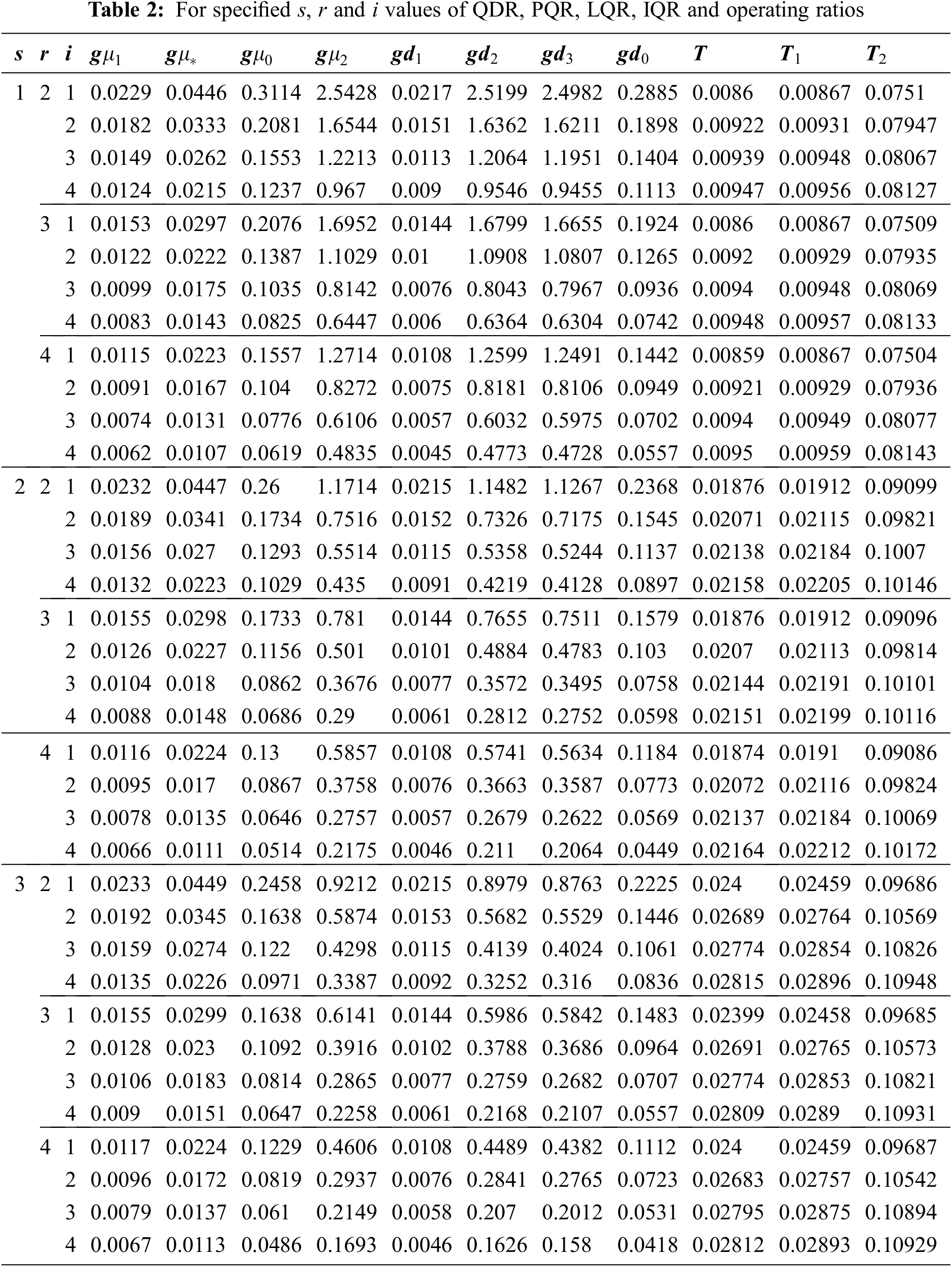
Given that μ1 = 0.01, r = 2, s = 2 and i = 4, compute the respective values of QDR, PQR, LQR, IQR, T, T1 and T2 from Tab. 2. The corresponding values are gd1 = 0.0091, gd2 = 0.4291, gd3 = 0.4128, gd0 = 0.0897 and the ratios T = 0.02158, T1 = 0.02205, T2 = 0.10146. From Tab. 1, the corresponding value of gμ1 = 0.0132 from which the required minimum number of groups can be obtained: g=gμ1μ1=0.01320.01=1.32≅2 . Thus, the selected parameters for BTSGChSP are r = 2, s = 2 and i = 4 with a minimum number of groups g = 2. Also, the values of QDR d1 = 0.0069, PQR d2 = 0.3251, LQR d3 = 0.3127, IQR d0 = 0.0680, and the ratios T = 0.02158, T1 = 0.02205, T2 = 0.10146.

3.1 For Specified QDR and PQR

When QDR and PQR are specified, then Tab. 2 is used to construct the plan for any values of d1 and d2 we can find the ratio T=d1d2 which is monotonic increasing function. Find the value which is equal to or just less than the specified ratio under column T in Tab. 2 and note the corresponding values of s, r and i. By this procedure, we can find all parameter values for BTSGChSP with a minimum number of groups g.

Suppose a manufacturing company required QDR d1 = 0.002 and PQR d2 = 0.07, then the calculated operating ratio is T = 0.02857. From Tab. 2, the value is just less than found to be T = 0.02815, with corresponding values of design parameters s = 3, r = 2 and i = 4. So, for this operating ratio gd1 = 0.0092 and gd2 = 0.3252, then the value of g=gd1d1=0.00920.002=4.6≅5 . Hence for the required QDR d1 = 0.002 and PQR d2 = 0.07 design parameters of BTSGChSP are s = 3, r = 2 and i = 4 with a minimum number of groups g = 5.

3.2 For Specified QDR and LQR

Let in a manufacturer company required QDR d1 = 0.002 and LQR d3 = 0.09, then the calculated operating ratio is T1 = 0.0222. From Tab. 2, the value is found to be T1 = 0.02212, with corresponding values of design parameters s = 2, r = 4 and i = 4. So, for this operating ratio gd1 = 0.0046 and gd3 = 0.2064, then the value of g=gd1d1=0.00460.002=2.3≅3 . Hence for the required QDR d1 = 0.002 and LQR d3 = 0.09 design parameters of BTSGChSP are s = 2, r = 4 and i = 4 with a minimum number of groups g = 3.

3.3 For Specified QDR and IQR

Let in a manufacturer company required QDR d1 = 0.01 and IQR d0 = 0.09, then the calculated operating ratio is T2 = 0.1111. From Tab. 2, the value is found to be T2 = 0.10948, with corresponding values of design parameters s = 3, r = 2 and i = 4. So, for this operating ratio gd1 = 0.0092 and gd0 = 0.0836, then the value of g=gd1d1=0.00920.01=0.92≅1 . Hence for the required QDR d1 = 0.01 and LQR d0 = 0.09 design parameters of BTSGChSP are s = 3, r = 2 and i = 4 with a minimum number of groups g = 1.

4  Graphs

Consider shape parameter s = 2 and number of testers r = 3, then for the number of preceding and succeeding lots i, j = 1, 2, 3, 4, the OC curves are shown in Fig. 3.

Figure 3: OC curves for i, j = 1, 2, 3, 4

Consider shape parameter s = 2, preceding and succeeding lots i = j = 3 are considered, then for the different number of testers r = 2, 3, 4, the OC curves are displayed in Fig. 4.

Figure 4: OC curves for r = 2, 3, 4

When the number of testers r = 4, preceding and succeeding lots i = j = 3 are considered, then OC curves for different values of shape parameters s = 1, 2, 3 are shown in Fig. 5.

Figure 5: OC curves for s = 1, 2, 3

From Figs. 3–5, we can conclude that the ideal OC curve can be achieved by increasing the value of the shape parameter, the number of testers and the number of preceding or succeeding lots.

For comparison purposes, BTSGChSP is compared with the existing BGChSP [12] for the same values of design parameters. For the specified design parameters, s = 2, r = 3 and i = j = 2, the average number of defectives is plotted against the average probability of acceptance in Fig. 6.

Figure 6: OC curves for BGChSP and BTSGChSP

From Fig. 6, it can conclude that the BTSGChSP OC curve is more ideal than the existing BGChSP [12]. For both plans, if the values of all design parameters are the same, BTSGChSP gives a smaller number of defectives than BGChSP.

5  Conclusion

The presented work in this paper is limited to BTSGChSP and four quality regions are estimated for the specified producer’s and consumer’s risks. This plan gives protection to both producer and consumer. Many electronic components such as transport electronics systems, wireless systems, global positioning systems, and computer-supported and integrated manufacturing systems can be evaluated by using the proposed plan. Many other distributions and other quality and reliability characteristics can be explored in the future.

Funding Statement: This research was supported by the Ministry of Higher Education (MoHE) through Fundamental Research Grant Scheme (FRGS/1/2020/STG06/UUM/02/2).

Conflicts of Interest: The authors declare that they have no conflicts of interest to report regarding the present study.

References

 1.  D. C. Montgomery, “Statistical Quality Control a Modern Introduction,” New York: John Wiley and Sons, Inc., 2009. [Google Scholar]

 2.  M. Latha and S. Jeyabharathi, “Performance measures for Bayesian chain sampling plan using binomial distribution,” International Journal of Advanced Scientific and Technical Research, vol. 1, no. 4, pp. 156–161, 2014. [Google Scholar]

 3.  B. Epstein, “Truncated life tests in the exponential case,” The Annals of Mathematical Statistics, vol. 1, no. 1, pp. 555–564, 1954. [Google Scholar]

 4.  H. F. Dodge, “Chain sampling plan,” Industrial Quality Control, vol. 11, no. 1, pp. 10–13, 1955. [Google Scholar]

 5.  A. Hald, “Bayesian single sampling plans for discrete prior distribution,” Danske Videnskabernes Selskab, vol. 3, no. 2, pp. 88, 1965. [Google Scholar]

 6.  M. Latha and K. K. Suresh, “Construction and evaluation of performance measures for Bayesian chain sampling plan (BChSP-1),” For East Journal of Theoretical Statistics, vol. 6, no. 2, pp. 129–139, 2002. [Google Scholar]

 7.  A. R. Mughal, M. Aslam, J. Hussain and A. Rehman, “Economic reliability group acceptance sampling plans for lifetimes following a Marshall-olkin extended distribution,” Middle Eastern Finance and Economics, vol. 7, pp. 87–93, 2010. [Google Scholar]

 8.  A. R. Mughal, Z. Zain and N. Aziz, “Economic reliability GASP for pareto distribution of the 2nd kind using poisson and weighted poisson distribution,” Research Journal of Applied Sciences, vol. 10, no. 8, pp. 306–310, 2015. [Google Scholar]

 9.  A. R. Mughal, Z. Zain and N. Aziz, “Time truncated group chain sampling strategy for pareto distribution of the 2(nd) kind,” Research Journal of Applied Sciences Engineering and Technology, vol. 10, no. 4, pp. 471–474, 2015. [Google Scholar]

10. A. R. Mughal, “A family of group chain acceptance sampling plans based on truncated life test,” Ph.D. dissertation, Universiti Utara Malaysia, Malaysia, 2018. [Google Scholar]

11. W. Hafeez and N. Aziz, “Bayesian group chain sampling plan based on beta binomial distribution through quality region,” International Journal of Supply Chain Management, vol. 8, no. 6, pp. 1175–1180, 2019. [Google Scholar]

12. W. Hafeez and N. Aziz, “Bayesian group chain sampling plan for poisson distribution with gamma prior,” Computers, Materials & Continua, vol. 67, no. 3, pp. 165–174, 2021. [Google Scholar]

13. K. Rosaiah and R. Kantam, “Acceptance sampling based on the inverse Rayleigh distribution,” Economic Quality Control, vol. 20, no. 2, pp. 277–286, 2005. [Google Scholar]

14. K. K. Suresh and V. Sangeetha, “Construction and selection of Bayesian chain sampling plan (BChSP-1) using quality regions,” Modern Applied Science, vol. 5, no. 2, pp. 226–234, 2011. [Google Scholar]

15. M. Latha and R. Arivazhagan, “Selection of Bayesian double sampling plan based on beta prior distribution index through quality region,” International Journal of Recent Scientific Research, vol. 6, no. 5, pp. 4328–4333, 2015. [Google Scholar]

This work is licensed under a Creative Commons Attribution 4.0 International License, which permits unrestricted use, distribution, and reproduction in any medium, provided the original work is properly cited.