Computer Systems Science & Engineering DOI:10.32604/csse.2023.025420
Article

Trend Autoregressive Model Exact Run Length Evaluation on a Two-Sided Extended EWMA Chart

Kotchaporn Karoon, Yupaporn Areepong* and Saowanit Sukparungsee

Department of Applied Statistics, King Mongkut's University of Technology, North Bangkok, Bangkok, 10800, Thailand
*Corresponding Author: Yupaporn Areepong. Email: yupaporn.a@sci.kmutnb.ac.th
Received: 23 November 2021; Accepted: 09 February 2022

Abstract: The Extended Exponentially Weighted Moving Average (extended EWMA) control chart is one of the control charts and can be used to quickly detect a small shift. The performance of control charts can be evaluated with the average run length (ARL). Due to the deriving explicit formulas for the ARL on a two-sided extended EWMA control chart for trend autoregressive or trend AR(p) model has not been reported previously. The aim of this study is to derive the explicit formulas for the ARL on a two-sided extended EWMA control chart for the trend AR(p) model as well as the trend AR(1) and trend AR(2) models with exponential white noise. The analytical solution accuracy was obtained with the extended EWMA control chart and was compared to the numerical integral equation (NIE) method. The results show that the ARL obtained by the explicit formula and the NIE method is hardly different, but the explicit formula can help decrease the computational (CPU) time. Furthermore, this is also expanded to comparative performance with the Exponentially Weighted Moving Average (EWMA) control chart. The performance of the extended EWMA control chart is better than the EWMA control chart for all situations, both the trend AR(1) and trend AR(2) models. Finally, the analytical solution of ARL is applied to real-world data in the health field, such as COVID-19 data in the United Kingdom and Sweden, to demonstrate the efficacy of the proposed method.

Keywords: Average run length; explicit formula; extended EWMA chart; trend autoregressive model

1  Introduction

The Control chart is one of the statistical process control instruments and has been applied in many fields such as finance, economics, industry, health, and medicine (see [1–5]). The concept of the control chart was initially introduced in 1931 by Shewhart [6]. The Shewhart control chart is more efficient in detecting large shifts in the processes. Next, the cumulative sum (CUSUM) [7] and the exponentially weighted moving average (EWMA) [8] control charts show that both are effective in detecting small shifts. After that, the EWMA control chart has been improved by many researchers, such as the modified exponentially weighted moving average (Modified EWMA) control chart that was originally presented by Patel et al. [9] and developed by Khan et al. [10]. These are effective in detecting small shifts quickly for observations with both autocorrelation and independently normal distribution. The extended exponentially weighted moving average (extended EWMA) control chart was proposed by Neveed et al. [11], and it is a good performance control chart for detecting small shifts in the monitored process.

The average run length (ARL) [12] can be used to evaluate the efficiency of control charts. It is divided into two states. For example, ARL0 is the expected number of observations before an in-control process is taken to signal to be out of control and should be large, whereas ARL1 is the expected number of observations taken from out of control and should be as small as possible. Previous research has shown that the ARL can be computed using various techniques. For instance, Areepong et al. [13] proposed the ARL by using the Martingale approach on the EWMA chart for exponential distribution. Chananet et al. [14] developed the ARL of the EWMA and CUSUM charts with a Markov chain approach based on the zero-inflated negative binomial (ZINB) model. Zhang et al. [15] proposed the ARL of a multivariate EWMA chart with Monte Carlo simulation. Karoon et al. [16] developed the numerical integral equation (NIE) method for evaluating the ARL on the extended EWMA chart for the AR(p) process.

There is a body of literature on evaluating the ARL with explicit formulas. Suriyakat et al. [17] derived the explicit formula for the ARL on the trend exponential AR(1) process in the EWMA chart. Phanyaem et al. [18] derived the ARL for the ARMA process via the explicit formula and the NIE method of the EWMA chart. Petcharat [19] analyzed the ARL by using the explicit formula on the EWMA chart for a seasonal moving average model of order q with exponential white noise. Sukparungsee et al. [20] solved the explicit formula of the ARL for the AR(p) model on the EWMA chart. Sunthornwat et al. [21] found the explicit formula and the optimal parameters to evaluate the ARL for a long-memory ARFIMA process on the EWMA chart. Recently, Supharakonsakun et al. [22] presented the exact solution of the ARL on the modified EWMA chart for the MA(1) process. Saghir et al. [23] proposed a modified EWMA chart that deduce the existing chart from its special cases. Aslam et al. [24] improved the Bayesian Modified EWMA location chart and its applications in the mechanical and sport industry. Phanthuna et al. [25] derived the explicit formula for the ARL on a modified EWMA chart for the trend stationary AR(1) model and a two-sided modified EWMA chart under the observations of AR(1) process [26]. Besides, the outbreak of COVID-19 has become a major problem facing humans all around the world. There are many literatures about control chart with the application to COVID-19 situation, such as Areepong et al. [27] derived by using quantile functions to monitor COVID-19 outbreaks via the EWMA chart based on the first hitting time of the total number of COVID-19 cases. Inkelas et al. [28] developed control charts at the country and city/neighborhood level within one state (California) to illustrate their potential value for decision-makers. However, the derivation of the explicit formula for the ARL on a two-sided Extended EWMA control chart for the trend AR(p) model has not been reported previously. Hence, the aim of this study is to derive the explicit formula of the ARL on a two-sided Extended EWMA control chart for the trend AR(p) model as well as the trend AR(1) and trend AR(2) models. The explicit formula for the ARL was compared with the NIE method for benchmarking. Furthermore, the explicit formulas capability for deriving the ARL on a two-sided Extended EWMA control chart was compared with the EWMA control chart for both simulated data and real-world data in the health field about COVID-19 data and compared.

2  Materials and Methods

2.1 Exponentially Weighted Moving Average (EWMA) Control Chart

The EWMA control chart was initially proposed by Roberts [8]. It is usually used to monitor and detect small shifts in the process. The EWMA statistic can be expressed as follows:

Zt=(1−λ)Zt−1+λXt,t=1,2,… (1)

where Xt is a process with mean, λ is an exponential smoothing parameter with λ ∈ (0, 1] and Z0 is the initial value of the EWMA statistic, Z0 = u. The upper control limit (UCL) and the lower control limit (LCL) are

UCL=μ+Lσλ2−λandLCL=μ−Lσλ2−λ (2)

where L is a suitable control limit width, μ is a process mean and σ is a process standard deviation.

The stopping time is given by

τa,h=inf{t≥0:Zt<a,Zt>h} (3)

where h is UCL and a is LCL.

2.2 Extended Exponentially Weighted Moving Average (Extended EWMA) Control Chart

The extended EWMA control chart was proposed by Neveed et al. [11]. It is developed from the EWMA control chart. That is a good performance control chart for detecting small shifts in the monitored process. The extended EWMA statistic can be expressed as follows:

Et=λ1Xt−λ2Xt−1+(1−λ1+λ2)Et−1,t=1,2,… (4)

where Xt is a process with mean, λ1 and λ2 are exponential smoothing parameters with λ1 ∈ (0, 1) and λ2 ∈ (0, λ1), E0 is the initial value of the extended EWMA statistic, E0 = u . The upper and lower control limits (UCL and LCL) are

UCL=μ0+Qσλ12+λ22−2λ1λ2(1−λ1+λ2)2(λ1−λ2)−(λ1−λ2)2andLCL=μ0−Qσλ12+λ22−2λ1λ2(1−λ1+λ2)2(λ1−λ2)−(λ1−λ2)2 (5)

where Q is a suitable control limit width, μ is a process mean and σ is a process standard deviation.

The stopping time is given by

τa,b=inf{t≥0:Et<a,Et>b} (6)

where b is UCL and a is LCL.

3  Analytical Solution of ARL on a Two-Sided Extended EWMA Chart for the Trend AR(p) Model

The observations equation for the autoregressive with trend or the trend AR(p) model in the case of exponential while noise is defined as

Xt=η+γt+ϕ1Xt−1+ϕ2Xt−2+⋯+ϕpXt−p+ϵtorXt=η+γt+∑i=1pϕiXt−i+ϵt (7)

where η is a suitable constant, γ is a slop, ϕi is an autoregressive coefficient at i = 1, 2, …, p such that |ϕp| < 1 and ɛt is white noise sequence of exponential (ɛt ∼ Exp(α)). The probability density function of ɛt is given by f(x)=1αe−xα where x ≥ 0. The extended EWMA statistics Et can be written as

Et=λ1(η+γt+∑i=1pϕiXt−i+ϵt)−λ2Xt−1+(1−λ1+λ2)Et−1

Et=λ1η+λ1γt+λ1∑i=1pϕiXt−i+λ1ϵt−λ2Xt−1+(1−λ1+λ2)Et−1

Et=λ1η+λ1γt+(1−λ1+λ2)Et−1+(λ1ϕ1−λ2)Xt−1+λ1∑i=2pϕiXt−i+λ1ϵt. (8)

If a and b are the lower and upper control limits of Et for in-control process, then a < Et < b.

Consequently, the extended EWMA statistics Et can be written as

a≤Et≤b

a<λ1η+λ1γt+(1−λ1+λ2)u+(λ1ϕ1−λ2)Xt−1+λ1∑i=2pϕiXt−i+λ1ϵt<b

a−λ1η−λ1γt−(1−λ1+λ2)u−(λ1ϕ1−λ2)Xt−1−λ1∑i=2pϕiXt−i<λ1ϵt<b−λ1η−λ1γt−(1−λ1+λ2)u−(λ1ϕ1−λ2)Xt−1−λ1∑i=2pϕiXt−i

a−λ1η−λ1γt−(1−λ1+λ2)u−(λ1ϕ1−λ2)Xt−1−λ1∑i=2pϕiXt−iλ1<ϵt<b−λ1η−λ1γt−(1−λ1+λ2)u−(λ1ϕ1−λ2)Xt−1−λ1∑i=2pϕiXt−iλ1

a−(1−λ1+λ2)u−(λ1ϕ1−λ2)Xt−1λ1−∑i=2pϕiXt−i−η−γt<ϵt<b−(1−λ1+λ2)u−(λ1ϕ1−λ2)Xt−1λ1−∑i=2pϕiXt−i−η−γt.

Let LE(u) denote the ARL on a two-sided extended EWMA control chart for the trend AR(p) model. The function LE(u) can be derived by Fredholm integral equation of the second kind [29], LE(u) is defined as follows:

LE(u)=1+∫L(E1)f(ϵ1)dϵ1 (9)

So, the function LE(u) is obtained as follows:

LE(u)=1+∫a−(1−λ1+λ2)u−(λ1ϕ1−λ2)Xt−1λ1−∑i=2pϕiXt−i−η−γtb−(1−λ1+λ2)u−(λ1ϕ1−λ2)Xt−1λ1−∑i=2pϕiXt−i−η−γtL(λ1η+λ1γt+(1−λ1+λ2)u+(λ1ϕ1−λ2)Xt−1+λ1∑i=2pϕiXt−i+λ1y)f(y)dy. (10)

Next step, Eq. (10) is changed by the variable of integration, and then LE(u) is obtained as:

LE(u)=1+1λ1∫abL(k)f(k−(1−λ1+λ2)u−(λ1ϕ1−λ2)Xt−1λ1−∑i=2pϕiXt−i−η−γt)dk. (11)

If ɛt ∼ Exp(α), then

LE(u)=1+e(1−λ1+λ2)u+(λ1ϕ1−λ2)Xt−1λ1α+∑i=2pϕiXt−i+η+γtαλ1α∫abL(k)e−kλ1αdk. (12)

when H(u)=e(1−λ1+λ2)u+(λ1ϕ1−λ2)Xt−1λ1α+∑i=2pϕiXt−i+η+γtα , K=∫abL(k)e−kλ1αdk .

Consequently,

LE(u)=1+H(u)λ1αK. (13)

Consider the constant K and take turn L(k) with Eq. (13),

K=−λ1α(e−bλ1α−e−aλ1α)1+1λ1−λ2⋅e(λ1ϕ1−λ2)Xt−1λ1α+∑i=2pϕiXt−i+η+γtα⋅(e−(λ1−λ2)bλ1α−e−(λ1−λ2)aλ1α). (14)

Substituting constant K form Eq. (14) into Eq. (13), then LE(u) can be written as

LE(u)=1−(λ1−λ2)e(1−λ1+λ2)uλ1α⋅(e−bλ1α−e−aλ1α)(λ1−λ2)e−{(λ1ϕ1−λ2)Xt−1λ1α+∑i=2pϕiXt−i+η+γtα}+(e−(λ1−λ2)bλ1α−e−(λ1−λ2)aλ1α). (15)

Finally, the solution of Eq. (15) is the explicit formula of ARL on a two-sided extended EWMA control chart for the trend AR(p) model. The process is in-control with the exponential parameter α = α0, whereas the process is out-of-control with the exponential parameter α = α1, and then α1 = (1 + δ)α0 where α1 > α0 and δ is the shift size.

4  NIE Method of ARL on a Two-Sided Extended EWMA Chart for the Trend AR(p) Model

The NIE method is one of the techniques that is used to approximate the ARL on a two-sided Extended EWMA chart for the trend AR(p) model. Let LN(u) be the estimated value of the ARL with the m linear equation systems by using the composite midpoint quadrature rule [16].

The ARL approximating NIE method on a two-sided extended EWMA chart is evaluated as follows:

∫abL(k)f(k)dk≈∑j=1mwjf(xj) (16)

The system of m linear equation is showed as:

Lm×1=1m×1+Rm×mLm×1or(Im−Rm×m)Lm×1=1m×1orLm×1=(Im−Rm×m)−11m×1

Lm×1=(Im−Rm×m)−11m×1,Lm×1=[LNIE(x1),LNIE(x2),…,LNIE(xm)]T,Im=diag(1,1,…,1)and1m×1=[1,1,…,1]T.

Let Rm×m be a matrix, the definition of the m to mth element of the matrix R is given by

[Rij]≈1λ1wjf(xj−(1−λ1+λ2)xi−(λ1ϕ1−λ2)Xt−1λ1−∑i=2pϕiXt−i−η−γt)

So, the solution of numerical integral equation can be explained as

LN(u)=1+1λ1∑j=1mwjL(xj)f(xj−(1−λ1+λ2)u−(λ1ϕ1−λ2)Xt−1λ1−∑i=2pϕiXt−i−η−γt) (17)

where xj is a set of the division point on the interval [a, b] as xj=(j−12)wj+a,j=1,2,…,m , wj is a weight of the composite midpoint formula wj=b−am .

5  Existence and Uniqueness of ARL

By using the Banach's Fixed-Point Theorem, the ARL solution demonstrates that the integral equation for explicit formulas exists only once. Let T be an operation in the class of all continuous functions.

T(LE(u))=1+1λ1∫abL(k)f(k−(1−λ1+λ2)u−(λ1ϕ1−λ2)Xt−1λ1−∑i=2pϕiXt−i−η−γt)dk (18)

If an operator T is a contraction, then the fixed-point equation T(LE(u)) = LE(u) has a unique solution. To show that Eq. (18) exists and has a unique solution, theorem can be used as follows below.

Theorem 1 Banach's Fixed-point Theorem: Let X be a complete metric space and T:X → X be a contraction mapping with contraction constant r ∈ [0, 1) such that ‖T(L1) − T(L2)‖ ≤ r‖L1 − L2‖, ∀L1,L2∈X . Then there exists a unique L( ⋅ ) ∈ X such that T(LE(u)) = LE(u), i.e., a unique fixed-point in X .

Proof: Let T defined in Eq. (18) is a contraction mapping for L1, L2 ∈ u[a, b], such that ‖T(L1) − T(L2)‖ ≤ r‖L1 − L2‖, ∀L1,L2∈u[a,b] with r ∈ [0, 1) under the norm ‖L‖∞=supu∈[a,b]⁡|L(u)| , so

‖T(L1)−T(L2)‖∞=supu∈[a,b]⁡|1λ1αe(1−λ1+λ2)u+(λ1ϕ1−λ2)Xt−1λ1α+∑i=2pϕiXt−i+η+γtα∫ab(L1(k)−L2(k))e−bλ1αdk|≤supu∈[a,b]⁡|‖L1−L2‖1λ1αe(1−λ1+λ2)u+(λ1ϕ1−λ2)Xt−1λ1α+∑i=2pϕiXt−i+η+γtα⋅(−λ1α)(e−bλ1α−e−aλ1α)|=‖L1−L2‖∞supu∈[a,b]⁡|e(1−λ1+λ2)u+(λ1ϕ1−λ2)Xt−1λ1α+∑i=2pϕiXt−i+η+γtα||e−aλ1α−e−bλ1α|≤r‖L1−L2‖∞

6  Comparing the ARL Results

According to Eq. (17), the ARL of the NIE method is approximated by division points m = 1,000 nodes. The solution of the NIE method is compared to the explicit formula for the trend AR(p) model on the extended EWMA chart by using the computation time (CPU time) and the absolute percentage relative error (APRE) [30], which can be computed as

APRE(%)=|LE(u)−LN(u)|LE(u)×100(19)

The speed test results were computed by the CPU time (PC System: windows10, 64-bit, Intel® Core™ i5-8250U 1.60, 1.80 GHz, RAM 4 GB) in seconds. In addition, the numerical results were computed by MATHEMATICA. The initial parameter value was studied at ARL0 = 370 on a two-sided extended EWMA chart for the trend AR(p) model namely the trend AR(1) and trend AR(2) models with exponential white noise and given λ1 = 0.05, λ2 = 0.01. The in-control process was presented a parameter value as α = α0 with shift size (δ = 0). On the other hand, the out-of-control process was presented parameter values as α1 = (1 + δ)α0 with shift sizes (δ = 0.001, 0.003, 0.005, 0.010, 0.030, 0.050, 0.100, 0.500, 1.000). Moreover, the coefficient parameters of the process (ϕ1 = 0.1, − 0.1) and (ϕ1 = 0.1, ϕ2 = 0.1, − 0.1) were used for the trend AR(1) model, and the trend AR(2) model, respectively. The process has determined that slope γ equals 0.1.

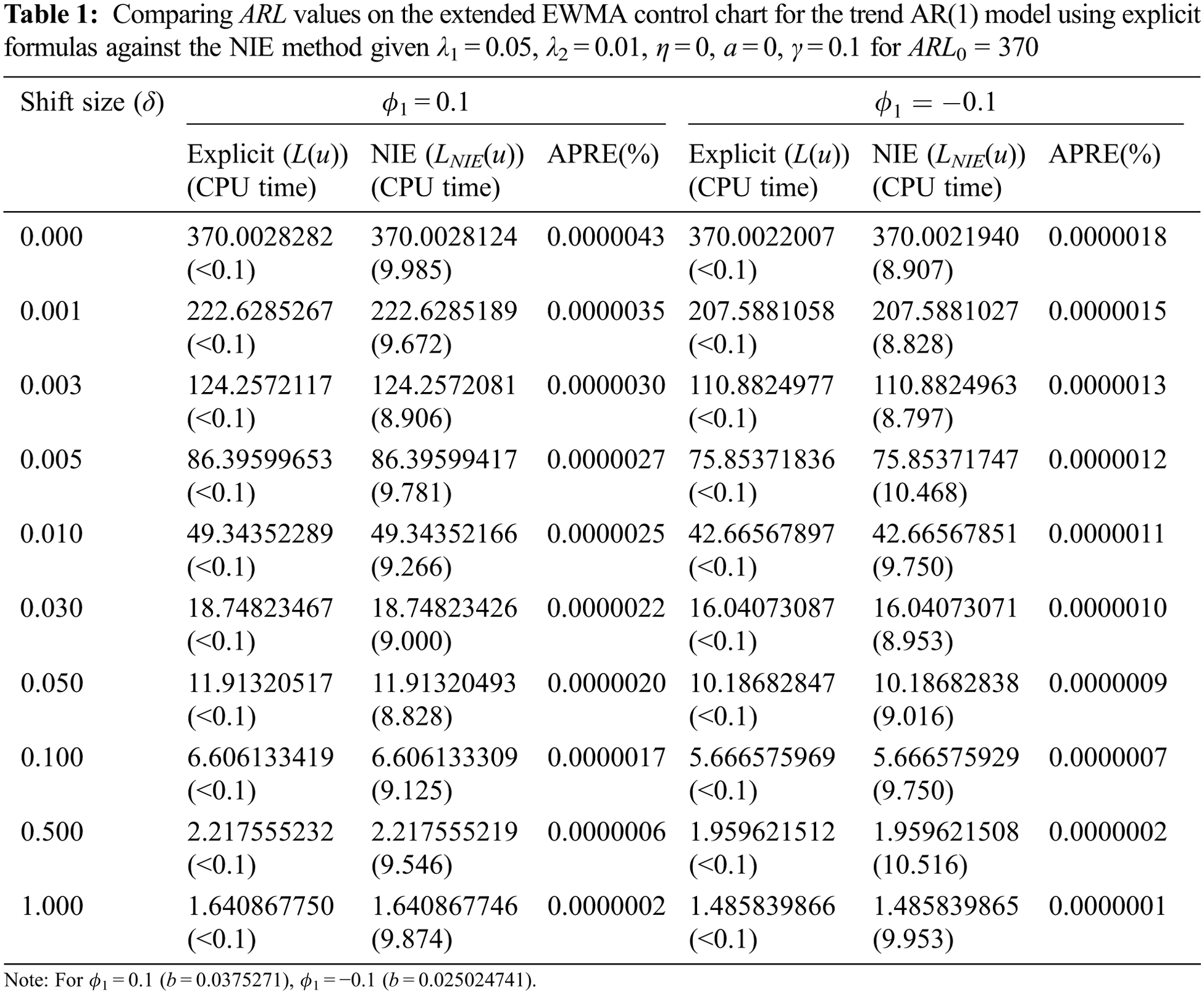
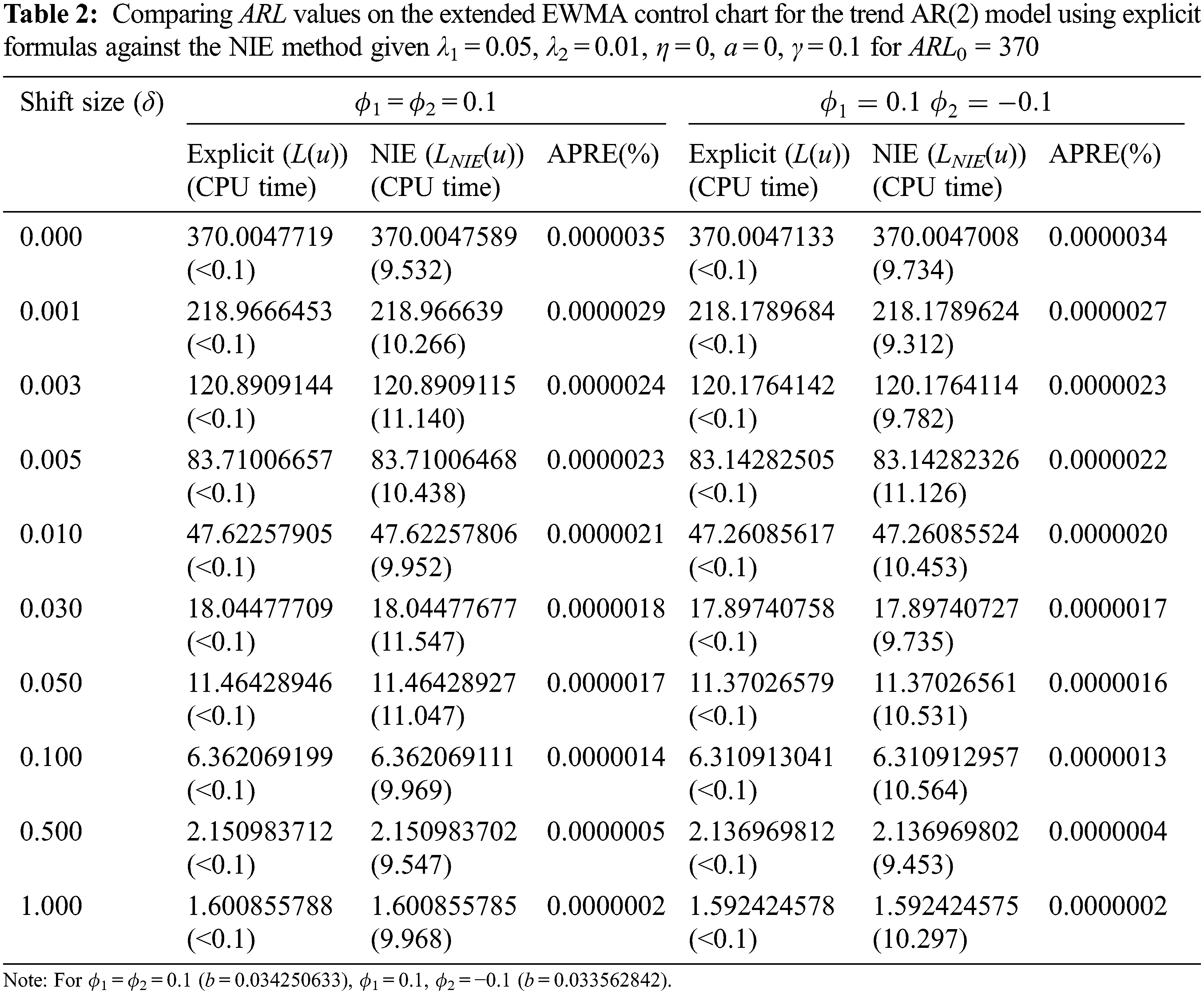
The performance comparisons of the explicit formula (as Eq. (15)) and NIE method (as Eq. (17)) are explained with ARL. In Tabs. 1 and 2, the ARL values derived from the explicit formula can help decrease the CPU time. The analytical results agree with NIE approximations with an APRE(%) less than 0.0000043% and 0.0000035%, and then the CPU time of approximately 8.8–10.5 and 9.3–11.5 s, for the trend AR(1) and trend AR(2) models, respectively, whereas the CPU time of the explicit formulas is less than 0.1 s, as well as the trend AR(1) and trend AR(2) models

7  Performance Comparing the ARL Results

The relative mean index (RMI) [31] is used to test the performance of a two-sided extended EWMA control chart on different bound control limits [a, b] and the comparative performance of the ARL under various λ conditions. The RMI can be computed as

RMI=1n∑i=1n[ARLi(c)−ARLi(s)ARLi(s)] (20)

where ARLi(c) is the ARL of the control chart for the shift size of row i, ARLi(s) is the smallest ARL of all of the control chart for the shift size of row i. The control chart's RMI value was the lowest, indicating that the control chart had the best performance at change detection.

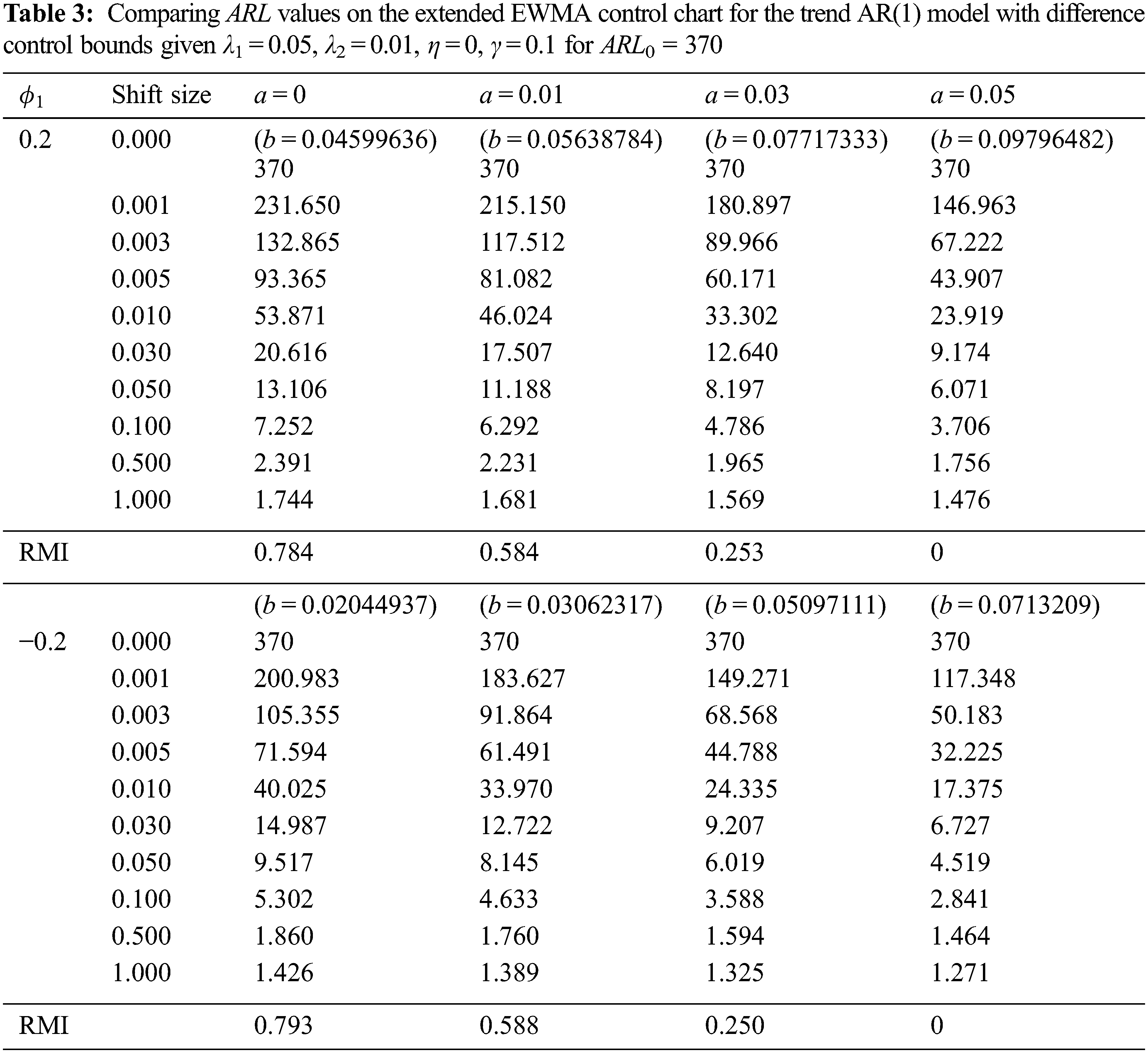
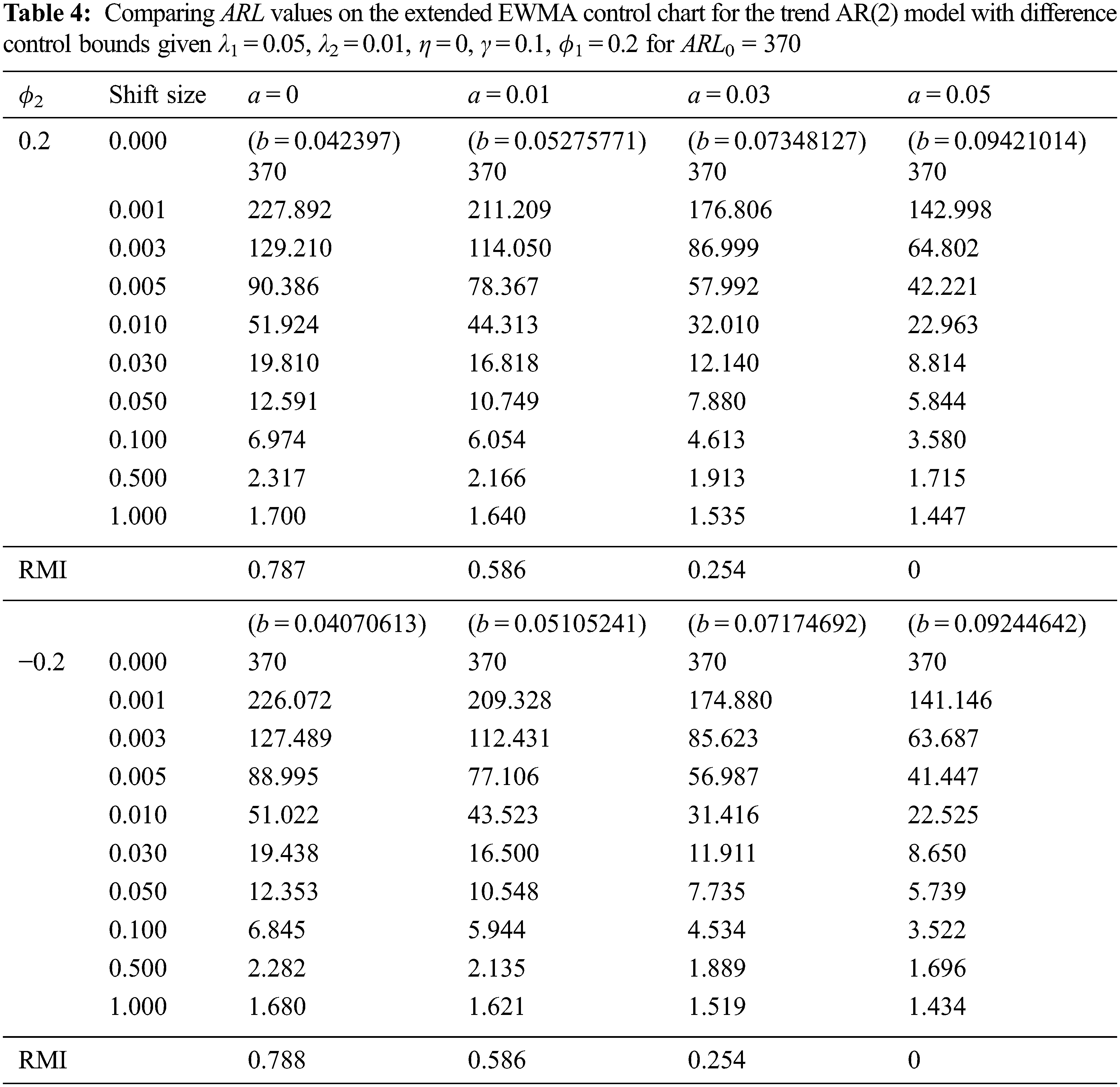
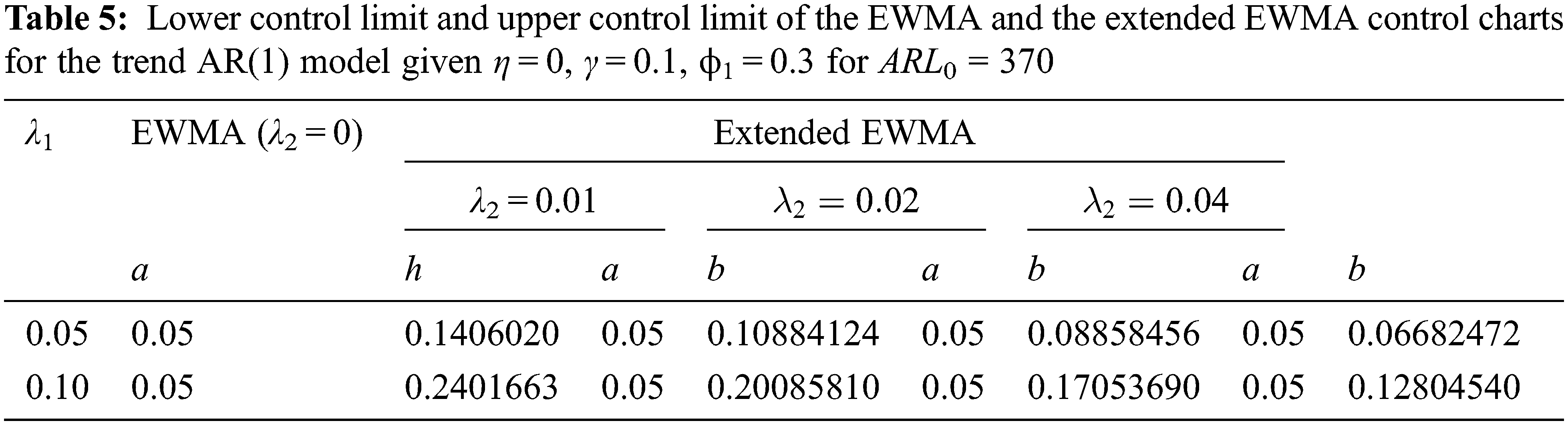
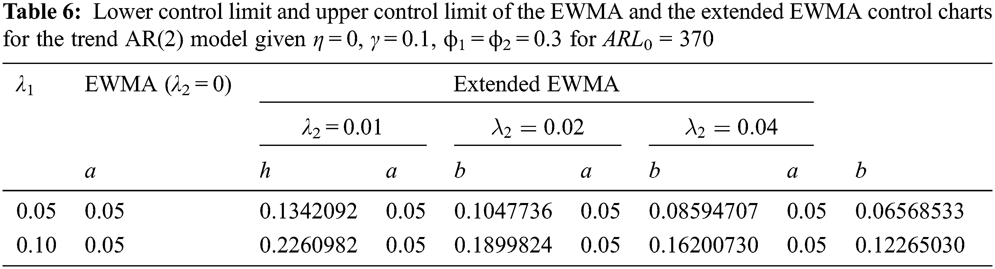
For Tabs. 3 and 4, the ARL results with λ1 = 0.05, λ2 = 0.01, γ = 0.1, η = 0 and ARL0 = 370 show that the performance of a two-sided extended EWMA control chart under various bound control limits [a, b], that were compared for, a = 0, 0.01, 0.03, 0.05 and ϕ1 = 0.2, − 0.2( as the trend AR(1) model) and ϕ1 = 0.2, ϕ2 = 0.2, − 0.2 (as the trend AR(2) model). The RMI values of the lower bound a = 0.05 are 0. The lower bound is higher indicated that the extended EWMA chart is more efficient for detecting shifts both two models.

Besides, a two-sided extended EWMA control chart under various conditions (λ2 = 0.01, 0.02, 0.04) are compared to the EWMA control chart (λ2 = 0) at λ1 = 0.05, 0.10, γ = 0.1, η = 0, a = 0.05 and ARL0 = 370 for ϕ1 = 0.3 (as the trend AR(1) model) and ϕ1 = ϕ2 = 0.3 (as the trend AR(2) model). The lower and upper control limits of the EWMA and extended EWMA control charts for the trend AR(1) and trend AR(2) models are obtained in Tabs. 5 and 6. The results in Tabs. 7 and 8 show that the RMI value of λ1 = 0.05 is equal to 0. The exponential smoothing parameter of 0.05 is recommended. In addition, the RMI results show that the extended EWMA chart with λ2 = 0.04(EEWMA0.04), (RMI = 0) had fewer RMI values than the extended EWMA chart with either λ2 = 0.01(EEWMA0.01) or λ2 = 0.02(EEWMA0.02) and the EWMA(λ2 = 0) control chart for all situations, both the trend AR(1) and the trend AR(2) models.

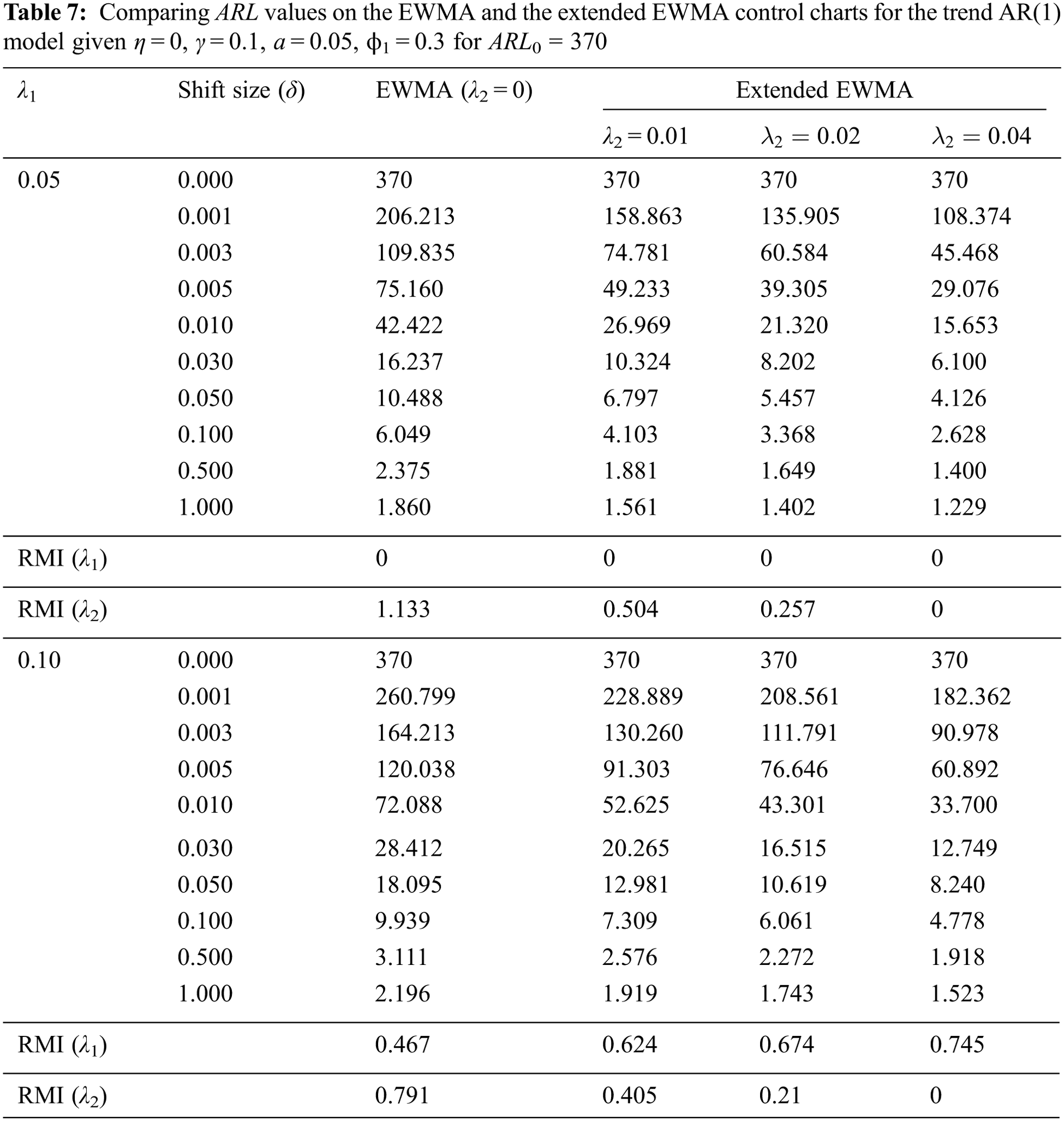
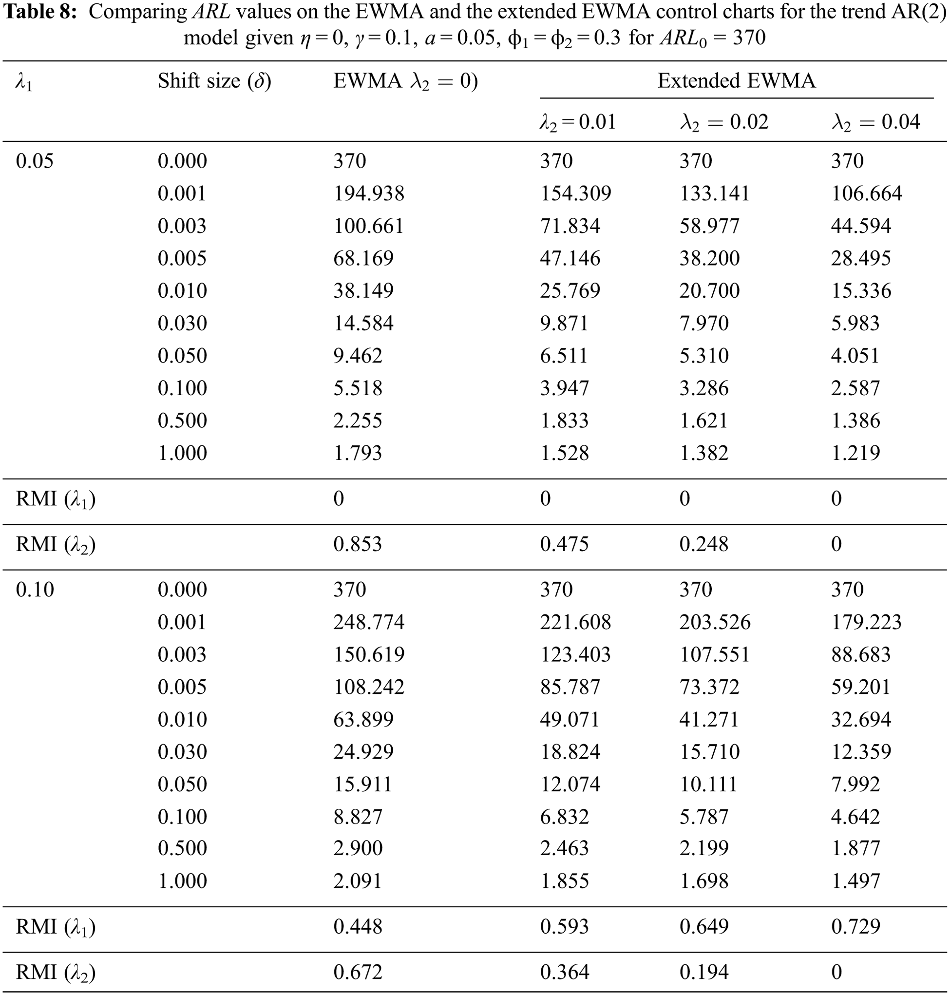
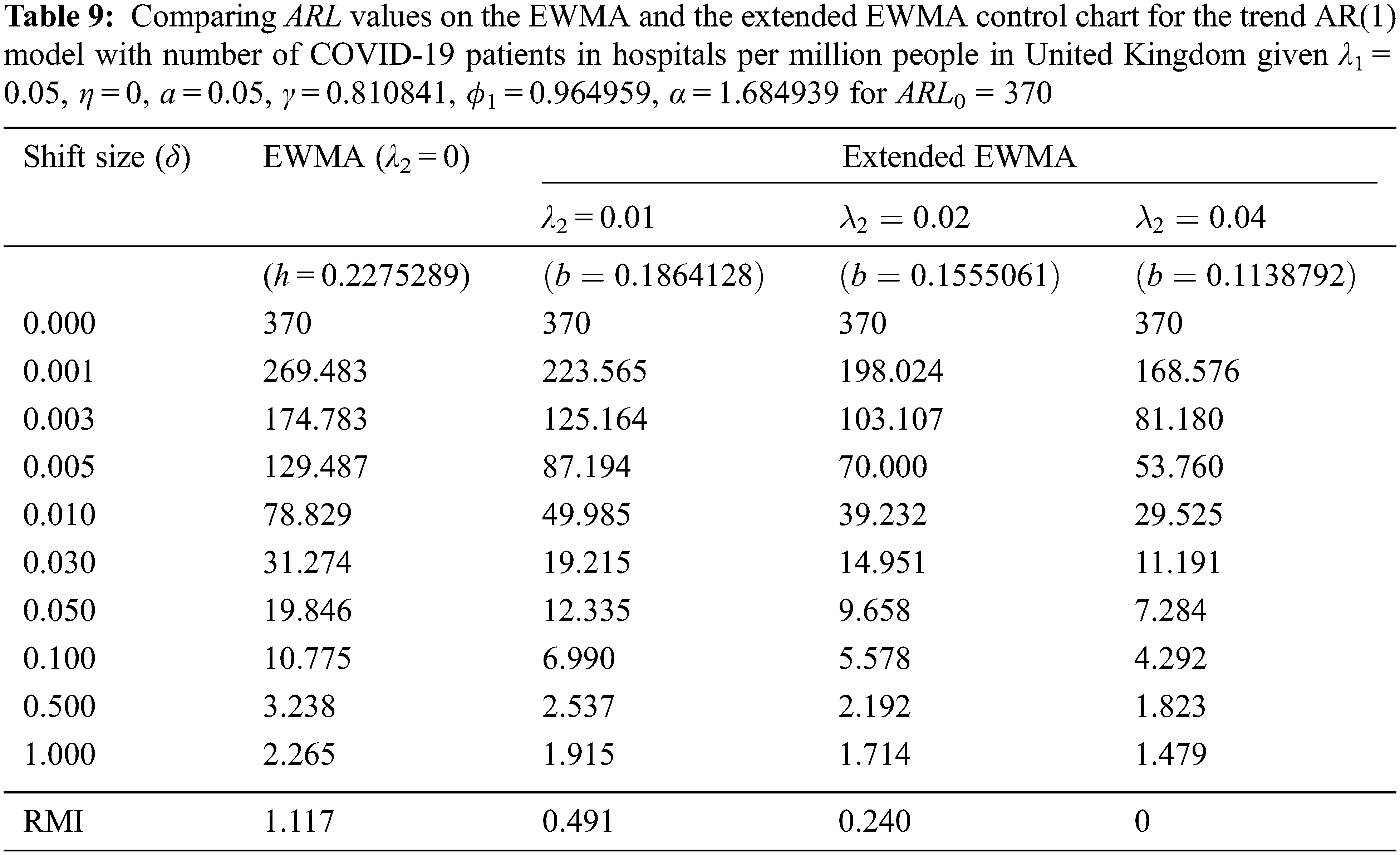
The results indicate that the performances of the control charts were, in ascending order, the extended EWMA with λ2 = 0.04, extended EWMA with λ2 = 0.02, extended EWMA with λ2 = 0.01 and EWMA control charts, as illustrated in Figs. 1 and 2.

Figure 1: ARL values on the EWMA and the extended EWMA control charts for the trend AR(1) model with ARL0 = 370; (a) λ1 = 0.05 and (b) λ1 = 0.10

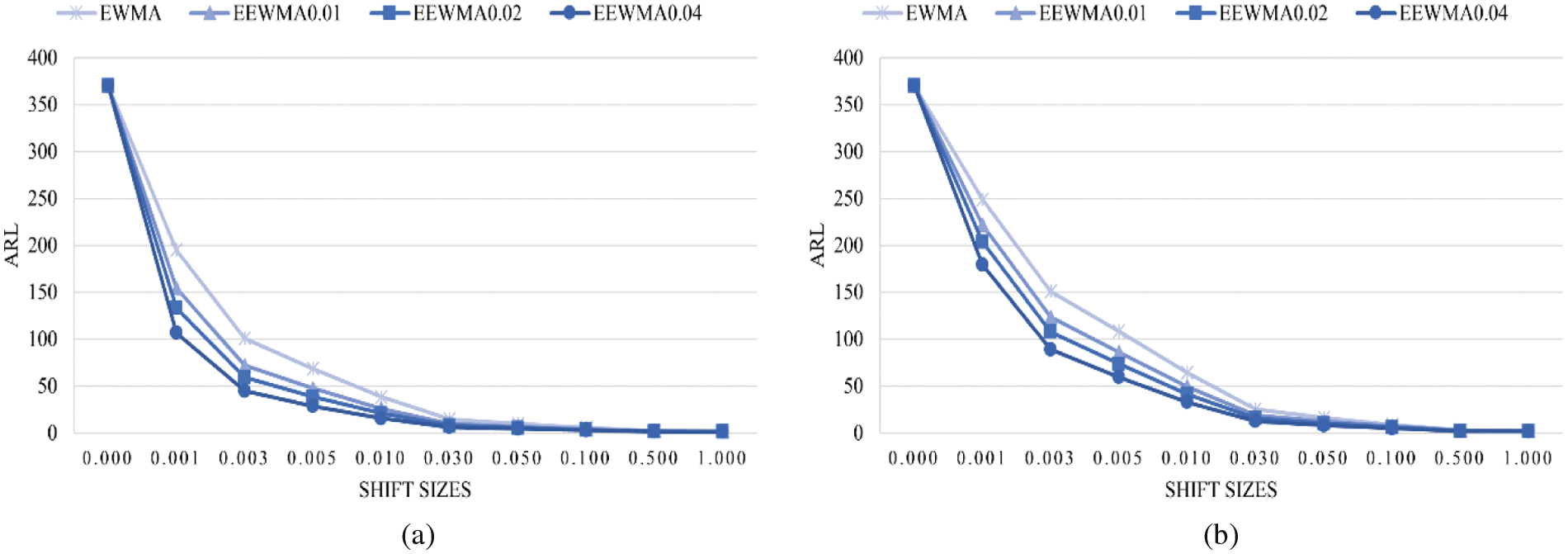
Figure 2: ARL values on the EWMA and the extended EWMA control charts for the trend AR(2) model with ARL0 = 370; (a) λ1 = 0.05 and (b) λ1 = 0.10

8  Application to Real Data

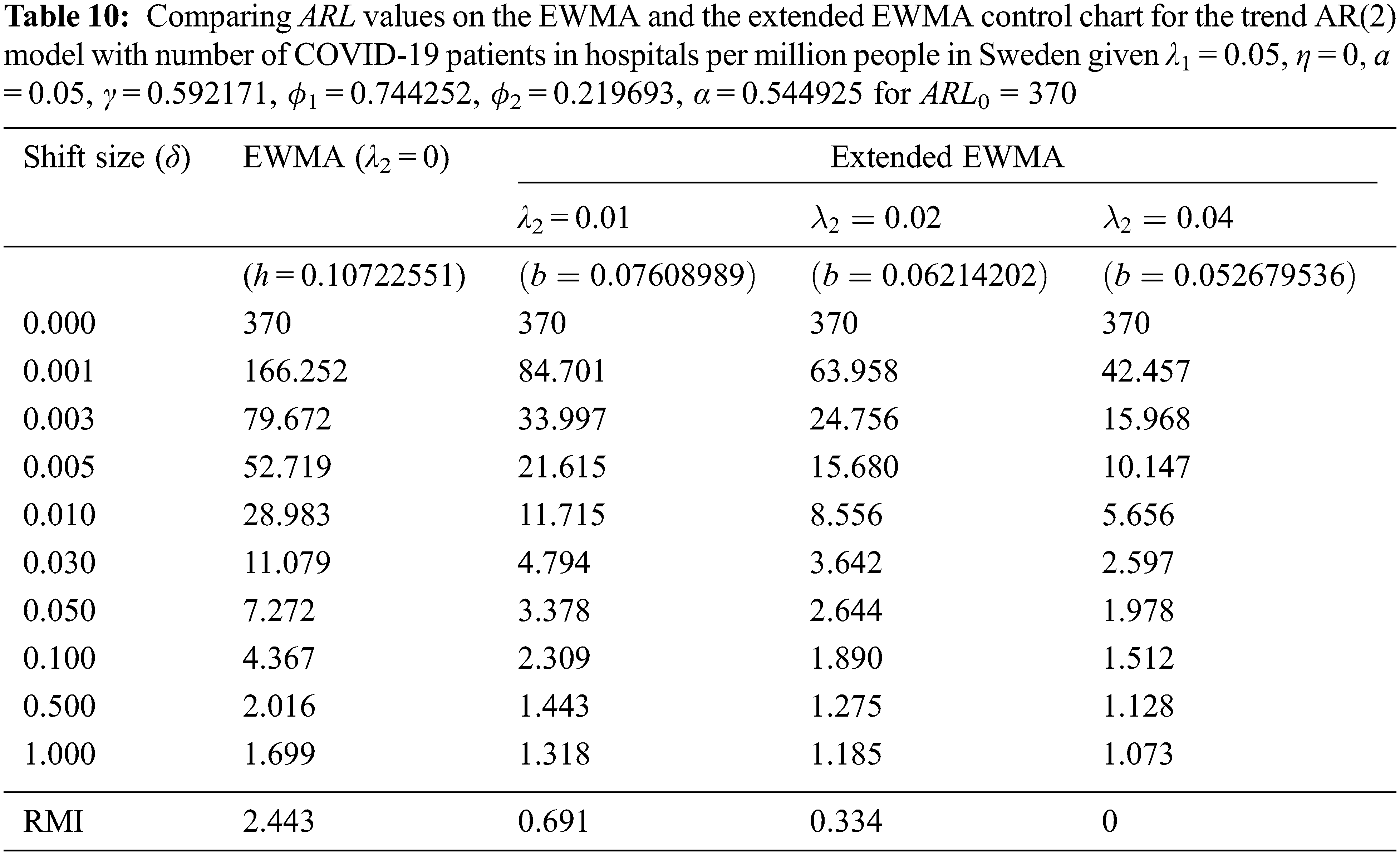
The ARL was constructed using explicit formulas on a two-sided extended EWMA control chart with ARL0 = 370 for λ1 = 0.05 and various λ2 = 0.01, 0.02, 0.04, and its performance was compared with the EWMA (λ2 = 0) control chart using data on the number of COVID-19 patients in hospitals per million people in the United Kingdom and Sweden. The observations were made daily from June 26th to September 10th, 2021 and from January 24th to April 20th, 2021, respectively. This data is a stationary time series by looking at the autocorrelation function (ACF) and partial autocorrelation function (PACF). The dataset for the trend AR(1) model was assigned as the significance of the mean and standard deviation were 79.32026 and 27.69376, respectively. The trend AR(p) model in Eq. (7), the observations of the trend AR(1) model was defined as Xt = (0.810841)t + (0.964959)Xt−1 + ɛt and the error was exponential white noise (α0 = 1.684939). Meanwhile, the observations of the trend AR(2) model was defined as Xt = (0.592171)t + (0.744252)Xt−1 + (0.219693)Xt−2 + ɛt and the error was exponential white noise (α0 = 0.544925). The RMI results show that the extended EWMA with λ2 = 0.04 chart reduced the RMI values more than the extended EWMA chart with either λ2 = 0.01 or λ2 = 0.02 and the EWMA control chart for all situations, both the trend AR(1) and trend AR(2) models. The results in Tab. 9 agree with the simulation results in Tab. 7. Similarly, the results in Tab. 10 agree with the simulation results in Tab. 8.

Hence, the extended EWMA (λ2 = 0.04) and EWMA (λ2 = 0) control charts were plotted by calculating Et and Zt for the two datasets when given λ1 = 0.05. Detecting the process with real data of the number of COVID-19 patients in hospitals per million people in the United Kingdom and Sweden were shown in Figs. 3 and 4, respectively. In Fig. 3, the ARL of the extended EWMA and EWMA control charts indicates that, the process was signaled as out-of-control at the 7th and 13th observations, respectively. In Fig. 4, the ARL of the extended EWMA and EWMA control charts indicates that the process was signaled as out-of-control at the 1st and 27th observations, respectively. As a result, a two-sided extended EWMA control chart can detect shifts faster than the EWMA control chart.

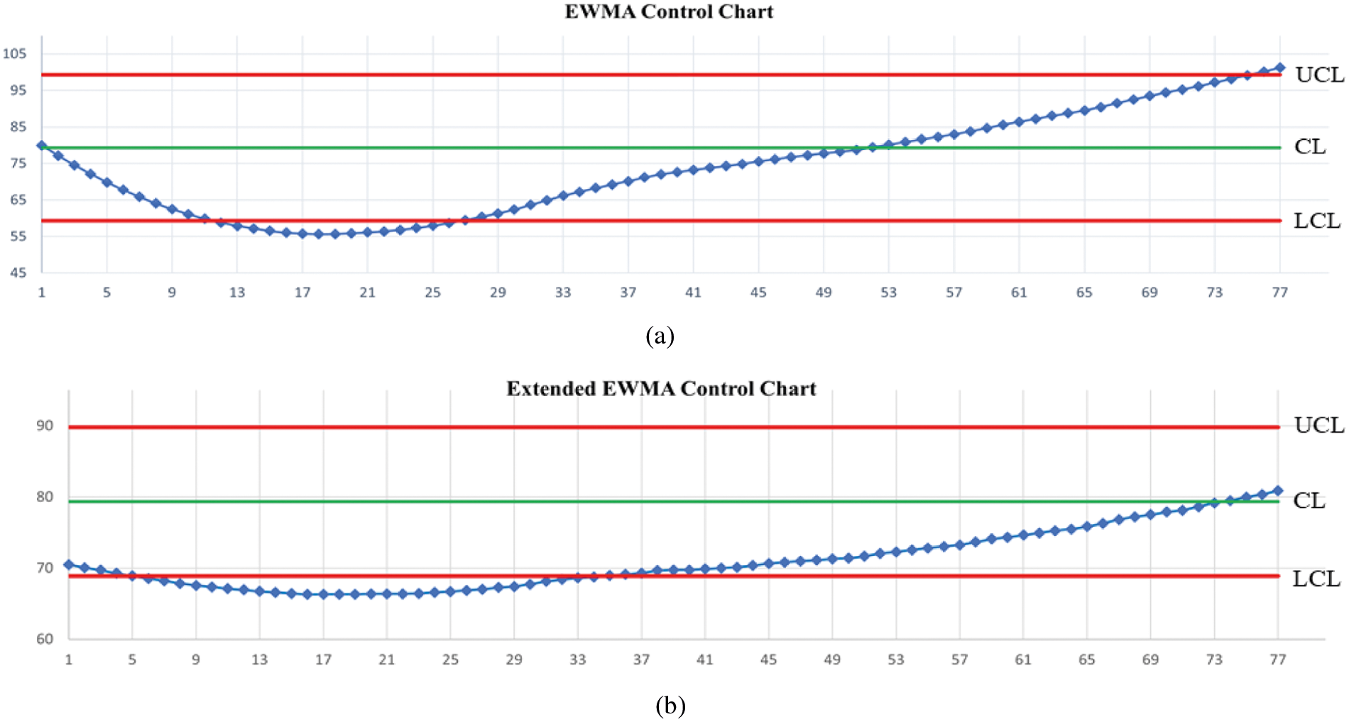
Figure 3: Detecting the number of COVID-19 patients in hospitals in the United Kingdom when given ARL0 = 370 under the trend AR(1) model on (a) EWMA chart and (b) Extended EWMA chart at λ2 = 0.04.

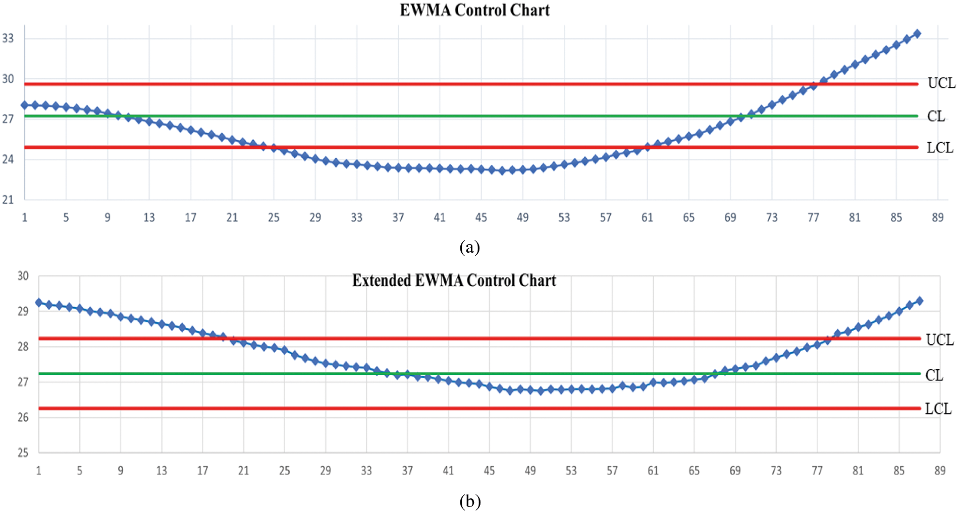
Figure 4: Detecting the number of COVID-19 patients in hospitals in Sweden when given ARL0 = 370 under the trend AR(2) model on (a) EWMA chart and (b) Extended EWMA chart at λ2 = 0.04.

9  Discussions and Conclusions

The performances of control charts were evaluated by using ARL. The explicit formulas comprise a good alternative to the NIE method for constructing the ARL, both the trend AR(1) and trend AR(2) models. The performance comparison of the ARL using explicit formulas on a two-sided extended EWMA on different bound control limits [a, b] and the comparative performance of the ARL under various λ conditions is further tested by using the relative mean index (RMI). The RMI values of the lower bound (a = 0.05) are 0. The extended EWMA control chart has given a higher capability for detecting shifts if the lower bound has been higher. When the comparative performance of the ARL under various λ1 conditions is examined, the RMI value with λ1 = 0.05 is equal to 0. So, the exponential smoothing parameter of 0.05 is recommended. Furthermore, the extended EWMA control chart has a higher efficiency if λ2 is increased. After that, the extended EWMA control can detect shifts faster than the EWMA control chart when the datasets were verified by calculating the control charts. Finally, the simulation study and the performance illustration with real data using data on the number of COVID-19 patients in hospitals per million people in the United Kingdom and Sweden provided similar results.

Acknowledgement: We are grateful to the referees for their constructive comments and suggestions which helped to improve this research.

Funding Statement: Thailand Science Research and Innovation Fund, and King Mongkut's University of Technology North Bangkok Contract No. KMUTNB-FF-65-45.

Conflicts of Interest: The authors declare that they have no conflicts of interest to report regarding the present study.

References

 1.  M. Kovarik and L. Sarga, “Implementing control charts to corporate financial management,” WSEAS Transactions on Mathematics, vol. 13, pp. 246–255, 2014. [Google Scholar]

 2.  M. Alsaid, R. M. Kamal and M. M. Rashwan, “The performance of control charts with economics-statistical design when parameters and estimated,” Review of Economics and Political Science, vol. 6, no. 2, pp. 142–160, 2021. [Google Scholar]

 3.  S. M. Anwar, M. Aslam, S. Ahmad and M. Riaz, “A modified-mxEWMA location chart for the improved process monitoring using auxiliary information and its application in wood industry,” Quality Technology and Quantitative Management, vol. 17, no. 5, pp. 561–579, 2020. [Google Scholar]

 4.  S. Ozigen, “Statistical quality control charts: New tools for studying the body mass index of populations from the young to the elderly,” The Journal of Nutrition, Health and Aging, vol. 15, no. 5, pp. 333–334, 2011. [Google Scholar]

 5.  S. H. Steiner, K. Grant, M. Coory and H. A. Kelly, “Detecting the start of an influenza outbreak using exponentially weighted moving average charts,” BMC Medical Informatics and Decision Making, vol. 10, no. 37, pp. 1–8, 2010. [Google Scholar]

 6.  W. A. Shewhart, Economic Control of Quality of Manufactured Product, NY, USA: Van Nostrand, 1931. [Google Scholar]

 7.  E. S. Page, “Continuous inspection schemes,” Biometrika, vol. 41, no. 1–2, pp. 100–115, 1954. [Google Scholar]

 8.  W. S. Roberts, “Control chart tests based on geometric moving averages,” Technometrics, vol. 1, no. 3, pp. 239–250, 1959. [Google Scholar]

 9.  A. K. Patel and J. Divecha, “Modified exponentially weighted moving average (EWMA) control chart for an analytical process data,” Chemical Engineering and Materials Science, vol. 2, pp. 12–20, 2011. [Google Scholar]

10. N. Khan, M. Alsam and C. H. Jun, “Design of a control chart using a modified EWMA statistics,” Quality and Reliability Engineering International, vol. 33, no. 5, pp. 1095–1104, 2017. [Google Scholar]

11. M. Neveed, M. Azam, N. Khan and M. Aslam, “Design a control chart using extended EWMA statistic,” Technologies, vol. 6, no. 4, pp. 108–122, 2018. [Google Scholar]

12. H. Khusna, M. Mashuri, S. Suhartono, D. D. Prastyo and M. Ahsan, “Multioutput least square SVR-based multivariate EWMA control chart: The performance evaluation and application,” Cogent Engineering, vol. 5, no. 1, pp. 1–14, 2018. [Google Scholar]

13. Y. Areepong and A. Novikov, “Martingale approach to EWMA control chart for changes in exponential distribution,” Journal of Quality Measurement and Analysis, vol. 4, no. 1, pp. 197–203, 2008. [Google Scholar]

14. C. Chananet, Y. Areepong and S. Sukparungsee, “A markov chain approach for average run length of EWMA and CUSUM control chart based on ZINB model,” International Journal of Applied Mathematics and Statistics, vol. 53, no. 1, pp. 126–137, 2015. [Google Scholar]

15. J. Zhang, Z. Li and Z. Wang, “Control chart based on likelihood ration for monitoring linear profiles,” Computational Statistics and Data Analysis, vol. 53, no. 4, pp. 1440–1448, 2009. [Google Scholar]

16. K. Karoon, Y. Areepong and S. Sukparungsee, “Numerical integral equation methods of average run length on extended EWMA control chart for autoregressive process,” in Proc. of Int. Conf. on Applied and Engineering Mathematics, London, England, pp. 51–56, 2021. [Google Scholar]

17. W. Suriyakat, Y. Areepong, S. Sukparungsee and G. Mititelu, “Analytical method of average run length for trend exponential AR(1) processes in EWMA procedure,” IAENG International Journal of Applied Mathematics, vol. 42, no. 4, pp. 250–253, 2012. [Google Scholar]

18. S. Phanyaem, Y. Areepong, S. Sukparungsee and G. Mititelu, “Explicit formulas of average run length for ARMA(1, 1),” International Journal of Applied Mathematics and Statistics, vol. 43, no. 13, pp. 392–405, 2013. [Google Scholar]

19. K. Petcharat, “Explicit formula of ARL for SMA(Q)L with exponential white noise on EWMA chart,” International Journal of Applied Physics and Mathematics, vol. 6, no. 4, pp. 218–225, 2016. [Google Scholar]

20. S. Sukparungsee and Y. Areepong, “An explicit analytical solution of the average run length of an exponentially weighted moving average control chart using an autoregressive model,” Chiang Mai Journal of Science, vol. 44, no. 3, pp. 1172–1179, 2017. [Google Scholar]

21. R. Sunthornwat, Y. Areepong and S. Sukparungsee, “Average run length with a practical investigation of estimating parameters of the EWMA control chart on the long memory AFRIMA process,” Thailand Statistician, vol. 16, no. 2, pp. 190–202, 2018. [Google Scholar]

22. Y. Supharakonsakun, Y. Areepong and S. Sukparungsee, “The exact solution of the average run length on a modified EWMA control chart for the first-order moving average process,” ScienceAsia, vol. 46, no. 1, pp. 109–118, 2020. [Google Scholar]

23. A. Saghir, M. Aslam, A. Faraz, L. Ahmad and C. Heuchenne, “Monitoring process variation using modified EWMA,” Quality and Reliability Engineering International, vol. 36, pp. 328–339, 2020. [Google Scholar]

24. M. Alsam and S. M. Anwar, “An improved bayesian modified EWMA location chart and its applications in mechanical and sport industry,” PLOS ONE, vol. 15, pp. e0229422, 2020. [Google Scholar]

25. P. Phanthuna, Y. Areepong and S. Sukparungsee, “Detection capability of the modified EWMA chart for the trend stationary AR(1) model,” Thailand Statistician, vol. 19, no. 1, pp. 70–81, 2021. [Google Scholar]

26. P. Phanthuna, Y. Areepong and S. Sukparungsee, “Exact run length evaluation on a two-sided modified exponentially weighted moving average chart for monitoring process mean,” Computer Modeling in Engineering and Sciences, vol. 1271, no. 1, pp. 23–40, 2021. [Google Scholar]

27. Y. Areepong and R. Sunthornwat, “EWMA control chart based on its first hitting time and coronavirus alert levels for monitoring symmetric COVID-19 cases,” Asian Pacific Journal of Tropical Medicine, vol. 14, no. 8, pp. 364–374, 2021. [Google Scholar]

28. M. Inkelas, C. Blair, D. Furukawa, V. G. Manuel, J. H. Malenfant et al., “Using control charts to understand community variation in COVID-19,” PLOS ONE, vol. 16, no. 4, pp. e0248500, 2021. [Google Scholar]

29. C. W. Champ and S. E. Rigdon, “A comparison of the markov chain and the integral equation approaches for evaluating the run length distribution of quality control charts,” Communications in Statistics-Simulation and Computation, vol. 20, no. 1, pp. 191–203, 1991. [Google Scholar]

30. Q. T. Nguyen, K. P. Tran, P. Castagliola, G. Celano and S. Lardiane, “One-sided synthetic control charts for monitoring the multivariate coefficient of variation,” Journal of Statistical Computation and Simulation, vol. 89, no. 1, pp. 1841–1862, 2019. [Google Scholar]

31. A. Tang, P. Castagliola, J. Sun and X. Hu, “Optimal design of the adaptive EWMA chart for the mean based on median run length and expected median run length,” Quality Technology and Quantitative Management, vol. 16, no. 4, pp. 439–458, 2018. [Google Scholar]

This work is licensed under a Creative Commons Attribution 4.0 International License, which permits unrestricted use, distribution, and reproduction in any medium, provided the original work is properly cited.