Computer Systems Science & Engineering DOI:10.32604/csse.2023.025594
Article

Big Data Analytics with Optimal Deep Learning Model for Medical Image Classification

Tariq Mohammed Alqahtani*

Department of Medical Equipment Technology, College of Applied Medical Sciences, Majmaah University, Al Majmaah, 11952, Saudi Arabia
*Corresponding Author: Tariq Mohammed Alqahtani. Email: talqahtani@mu.edu.sa
Received: 29 November 2021; Accepted: 09 February 2022

Abstract: In recent years, huge volumes of healthcare data are getting generated in various forms. The advancements made in medical imaging are tremendous owing to which biomedical image acquisition has become easier and quicker. Due to such massive generation of big data, the utilization of new methods based on Big Data Analytics (BDA), Machine Learning (ML), and Artificial Intelligence (AI) have become essential. In this aspect, the current research work develops a new Big Data Analytics with Cat Swarm Optimization based deep Learning (BDA-CSODL) technique for medical image classification on Apache Spark environment. The aim of the proposed BDA-CSODL technique is to classify the medical images and diagnose the disease accurately. BDA-CSODL technique involves different stages of operations such as preprocessing, segmentation, feature extraction, and classification. In addition, BDA-CSODL technique also follows multi-level thresholding-based image segmentation approach for the detection of infected regions in medical image. Moreover, a deep convolutional neural network-based Inception v3 method is utilized in this study as feature extractor. Stochastic Gradient Descent (SGD) model is used for parameter tuning process. Furthermore, CSO with Long Short-Term Memory (CSO-LSTM) model is employed as a classification model to determine the appropriate class labels to it. Both SGD and CSO design approaches help in improving the overall image classification performance of the proposed BDA-CSODL technique. A wide range of simulations was conducted on benchmark medical image datasets and the comprehensive comparative results demonstrate the supremacy of the proposed BDA-CSODL technique under different measures.

Keywords: Big data analytics; healthcare; deep learning; image classification; biomedical imaging; machine learning

1  Introduction

Big data originally demonstrates the variety, volume, and velocity of data acquired during different data production times. Medical big data, acquired at healthcare providers, contains data relevant to patient care such as diagnoses, demographics, medications, medical procedures, immunizations, vital signs, radiology images, laboratory results and so on [1]. With technological improvements made in medical data collection through healthcare devices, automated healthcare resources like streaming machines, high throughput instruments, and sensor devices have increased. This sort of health care big data has different applications to its credit such as drug discovery, diagnosis, disease prediction, precision medicine, and so on. Big data plays a significant role in several environments like scientific research, healthcare, social networking, public administration, industry etc., [2]. Big data can be determined by 5Vs. When big data is leveraged appropriately, it provides a wide range of novel opportunities for widening the knowledge base and creating advanced techniques to enhance the quality of healthcare. Few important applications of healthcare big data are medical operation, research and development, public healthcare, remote monitoring, evidence-based medicine, patients profile analysis, and so on. Big Data Analytics (BDA) is the application of innovative analytical methods against extremely complicated large datasets including structured, unstructured, and semi-structured data, collected from various resources, in varying sizes from terabytes to zettabytes [3]. In terms of healthcare, BDA encompasses analytics and integration of a huge number of complicated heterogeneous data like different—omics data (epigenomics, genomics, pharmacogenomics, transcriptomics, metabolomics, diseasomics, proteomics, interactomics), EHR (Electronic Health Record), and biomedical data. Amongst these, EHR plays an important role in today's healthcare settings and is being currently adopted across several countries [4]. The primary objective of EHR is to obtain actionable big data insight from healthcare workflows.

The huge amount of health care data constitute the images acquired through medical imaging techniques (Echography, Computed Tomography Scan, MRI, Mammography, and so on.). In order to perform a comprehensive analysis and achieve biomedical image management, each step in healthcare process should be automated [5]. When image classification is executed appropriately, it produces better and automated diagnosis of the disease from the captured image. The diagnostic algorithm can adopt consequently to the image group which results in classification. Hence, classification is one of the key steps in biomedical automation scheme [6]. Machine Learning is one of the artificial intelligence methods which represents the capacity of IT system to individually find solutions for the problems through identification of patterns in datasets. ML algorithm allows the IT systems to identify patterns according to the present algorithm and datasets. Afterwards, it improves the concept of satisfactory solution. Thus, in ML techniques, artificial knowledge is created on the basis of experience. Mathematical and statistical models are applied in ML to learn from datasets. There are two major methods followed in ML techniques such as symbolic approach and sub-symbolic approach [7]. Symbolic system is otherwise called as propositional system in which the knowledge content i.e., induced rules and instances are explicitly represented. While, sub-symbolic system is otherwise named as artificial neuronal network that works on the principle of human brain i.e., here, the knowledge content is implicitly represented. Machine Learning techniques face key challenges such as high-speed streaming data, largescale data, distinct kinds of data, incomplete and uncertain data [8].

ML and DL methods (i.e., CNN, SVM, and NN) have attained outstanding performances in biomedical image classification [9]. Classification process assists in a wide range of processes such as organization of biomedical image databases to image classifications, before diagnostics. Several researches have been conducted earlier to improve the quality of biomedical image classification.

In this background, the current study presents a new Big Data Analytics with Cat Swarm Optimization based Deep Learning (BDA-CSODL) technique for medical image classification on Apache Spark environment. The proposed BDA-CSODL technique involves Bilateral Filtering (BF)-based noise removal technique as a preprocessing step. Moreover, the proposed BDA-CSODL technique involves multi-level thresholding-based image segmentation too with deep convolutional neural network-based Inception v3 technique as a feature extractor. Furthermore, Stochastic Gradient Descent (SGD) model is used for parameter tuning process. Finally, CSO with Long Short-Term Memory (CSO-LSTM) method is utilized as a classifier to allot proper class labels to it. In order to showcase the improved performance of the proposed BDA-CSODL technique, a comprehensive experimental analysis was conducted against benchmark medical images.

2  Literature Review

In Ashraf et al. [10], a new image depiction algorithm was presented. In this study, the model is trained to classify the medicinal images by following DL approaches. A pre-trained DCNN model is employed for last three layers of DNN model using the fine-tuned approaches. The experimental result showed that this approach is appropriate for the classification of different medical images for different body parts. Yadav et al. [11] employed a CNN-based method on chest X-ray datasets for the classification of pneumonia. Three methods were evaluated in this study that include linear SVM classifiers using orientation-free and local rotation features, TL on two CNN methods: Visual Geometry Group viz., InceptionV3 and VGG16, and a capsule network training from scratch. In this study, data augmentation, a data pre-processing model was also employed for all three models.

In Tan et al. [12], a new multimodal medicinal image fusion method was presented to overcome a broad variety of medicinal diagnostic problems. This method is based on the application of energy attribute fusion approach and boundary-measured pulse-coupled NN fusion approach in a non-subsampled shearlet transform domain. The researchers authenticated the method using a dataset of various diseases, i.e., metastatic bronchogenic carcinoma, glioma, and Alzheimer's, that contains over 100 image pairs. In Gao et al. [13], a new technique was presented to enable the DL algorithm for optimal learning of single-class relevant inherent imaging features by leveraging difficult imaging concept. The study compared and investigated the effect of simple, yet efficient perturbing operation employed to capture complex images and to improve feature learning.

Wang et al. [14] presented a self-training method on the basis of repeated labelling approach to resolve the mislabeled instance problems since it weakens the performances of the classifier. Aimed at achieving medicinal data management, this study extracted the features with higher relation of classification result. According to the domain expert's knowledge, the unlabeled medicinal record data is selected later with high confidence to extend the training set. Then the performances of the classifier of tri-training model that employs supervised learning model for training three fundamental classifications, is optimized. Zhang et al. [15] introduced different ResNet models by exchanging global average pooling with an adoptive dropout for medicinal image classification. The aim is to identify various diseases (viz., multilabel classifications). Then, multilabel classifications are transformed to N binary classification by training the parameters of the proposed method for N times.

3  The Proposed Model

In this study, a new BDA-CSODL technique is presented for biomedical image classification on Apache Spark environment. The proposed BDA-CSODL technique encompasses BF-based preprocessing, Otsu-based segmentation, Inception v3-based feature extraction, SGD-based hyperparameter optimization, LSTM-based classification, and CSO-based parameter tuning. Fig. 1 depicts the overall processes involved in the proposed BDA-CSODL model. The presented BDA-CSODL technique is executed on Apache Spark environment whereas the detailed working mechanisms of these processes are discussed herewith.

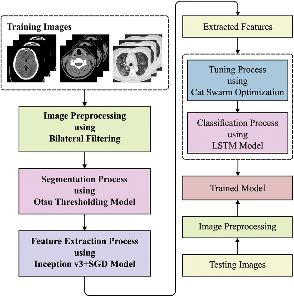
Figure 1: Overall processes involved in BDA-CSODL model

3.1 Modeling of Spark Environment

Apache Spark is a distributed computing system utilized in big data environment and is the most effective framework developed in this regard. Spark provides a complete and unified structure for managing differential needs to big data processing with different types of datasets (text data, graph data, image/video, and so on.) collected from various sources (realtime streaming, batch, etc.). Spark has been developed to resolve the problem encountered in Hadoop frameworks. Indeed, Spark frameworks have demonstrated its fast-execution potentials than Hadoop frameworks under different scenarios (over 100 times in memory).

Apache Spark framework involves several phases as shown in Fig. 2. The key role of the feature in image biomedical classification is to convert visual data into vector space so that it could execute mathematical models on them and detect the same vector. In feature selection process, the basic challenge is to find the feature on biomedical images [16].

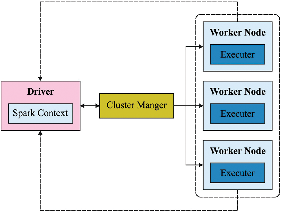
Figure 2: Apache spark structure

Since the number of features could be dissimilar based on the image, some clauses can be included so as to make these feature vectors are of similar size. Next, vector descriptors are constructed according to this feature; all the descriptors are of similar size. In this method, it has to be pointed out that the feature extraction from labeled/unlabeled images is executed by several images in big data context, regarding distinct V's of big data (velocity, volume, variability, veracity, and variety). But the performance of Spark algorithm gets reduced at few scenarios, particularly during feature extraction when few smaller images exist under the datasets (labeled biomedical images or unlabeled biomedical image). In order to resolve this problem, the researchers proposed two approaches such as feature extraction by segmentation and sequence in feature extraction. The performance of one of these two approaches could solve the problems faced in unbalanced loading, while the execution time of every task could be a similar process. The classification procedure is initiated, once the novel unlabeled data comes to the scheme.

In this method, both query and prediction are implemented during MapReduce stage itself. The adoption of Spark frameworks comes with advantage to process in a big data platform and uses their embedding libraries, for instance MLlib (Machine Learning library).

3.2 BF-Based Preprocessing

For a non-linear, edge preserving image filtering model, BLF treats the intensity values of all the pixels as weighted average of its adjacent pixels’ intensity value [17]. BLF can resolve Gaussian blur problems faced in conventional Gaussian convolution-based image filter method, since it integrates two modules such as radiometric difference and Euclidean distance which is formulated herewith.

D(p)=kp−1∑q∈RP⁡Ws(dpq)Wr(fpq)I(q) (1)

kp=∑q∈RP⁡Ws(dpq)Wr(fpq) (2)

Here,  I(q) & D(p) denote the image intensity of pixel q in input image and pixel p in output image, correspondingly. Rp represents a collection of pixels adjacent to pixel p.Wr & Ws denote range kernel and spatial kernel respectively whereas the weight is calculated from photometric difference fpq and Euclidean distance dpq between the pixels, q and p, correspondingly. The latter is generally calculated with image features like texture/intensity. kp−1 is a standardization term calculated using (2). In (1), Wr and Ws take an inverse value to the equivalent input and is formulated normally as a Gaussian function. For instance, Ws is computed as follows.

Ws(dpq)=exp(−dpq22σs2) (3)

In (3), σs represents the scale variables that determine the weight distribution patterns of the kernel. A large σs implies that the Gaussian range fattens as well as widens.

3.3 Multi-level Thresholding Based Segmentation

Next to preprocessing, Otsu technique is employed to segment the medical images and determine the affected regions. Otsu is a generally-employed image thresholding method that was originally proposed by Otsu in 1979. At present, Otsu criterion is commonly used in defining the optimum threshold model which can offer histogram-based image segmentation using acceptable results. For simple bi-level threshold, the original method in Otsu can be determined as following: initially, an image is assumed to have N pixel of grey level from 0  to L − 1. The numbers in ith gray level pixels is represented by h(i), & PRi represents the likelihood of i. Next, the grey level histogram for an image can be standardized and determined as given herewith.

PRi=hiN,0≤i≤t,t+1≤i≤L−1 (4)

When the threshold is t, the original images are categorized under two groups such as C0 & C1:C0 for [0, …, t],C1 , for [t+1, …, L−1].  The increasing probability of class existence can be stated as follows.

ω0=P(C0)=∑i=1t⁡PRi,  ω1=P(C1)=∑i=t+1L−1⁡PRi (5)

The mean intensity values for bi-level threshold of all the classes are shown in the following equation

μ0=∑i=0t⁡iPRiω0,  μ1=∑i=t+1L−1⁡iPRiω1 (6)

After calculating this value, class variance σB2 is determined as follows.

σB2=σ02+σ12 (7)

Whereas σ02 & σ12 represent the variances of C0 & C1 correspondingly which are determined as given herewith.

σ02=ω0(μ0−μT)2,  σ12=ω1(μ1−μT)2 (8)

Whereas μT denotes the overall mean intensity of original images determined by μT = ω0μ0 + ω1μ1 and ω0 + ω1 = 1. Based on the aforementioned analyses [18], the class variance depends on a binary classification as expressed in the following equation:

σB2(t∗)=max{σB2(t)},  0≤t≤L−1 (9)

Eqs. (5) to (9) are used to determine bi-level threshold problems and are easily expanded to multi-level threshold of the images as follows.

σB2(t1∗, t2∗, …, tn−1∗)=max{σB2(t1, t2, …, tn−1)} (10)

Whereas 1 ≤ t1 < t2 < ⋅ ⋅ ⋅ < tn−1 < L.

3.4 Inception v3 Based Feature Extraction

During feature extraction, Inception v3 model is executed to produce a useful set of feature vectors. In line with GoogLeNet (Inception-v1), Inception-v3 has progressed well in recent years with each update being incorporated in Inception-v2. During classification, LSR (Label Smoothing Regularization) is included after fully-connected layers. In convolution layer, 7 × 7 kernels are substituted by 3 × 3 kernels. Also, regularization is utilized and normalization is included in loss function to avoid overfitting. Initially, three convolution layers, two pooling layers, one pooling layer and two convolution layers are fixed. At last, elven dropout layer, mixed layers, softmax layer, and fully connected layer are followed. Padding and convolution operations are performed continuously on the images, in all the layers [19]. Then, data conversion is proposed. Beforehand softmax layer, the images are transformed to 2,048 dimensional vectors. At many instances of applying machine learning techniques, the method is determined from the scratch although a method already exists based on equivalent data. The continuous development of new methods drains the resources. Taking the comparison of distinct methods into account and based on the knowledge acquired so far, TL method can be employed for establishing novel models. In the meantime, there have been two challenges experienced in DL training models; the data is frequently inadequate and the computational becomes slower. But, great performances can be achieved from small data and pre-trained models. The TL model can determine many such novel models based on the relationship between target and source domains.

Since hyperparameter tuning process affects the classification performance considerably, it is performed using SGD optimizer. With reference to determination of mean variance portfolio optimization problems, an augmented objective function fa(w) can be defined as follows.

fa(w)=12wTΣw+λ1(R−wTμ)+λ2(1−wT1)+λ3TW (11)

with w=(w1, …,wn)T . As far as the presence of uncertainty is concerned, the augmented objective function fa(w), determined in (11), is expressed as the projected objective function,

E[fa(w)]=1n∑i=1n⁡fa,i(w) (12)

Whereas fa,i(w),  i = 1, …, n, represents the augmented objective function fa(w) component which is uniformly sampled while E [•] denotes the expectation operator. According to this, the sampled gradient ∇fa,i(w) is represented as un-biased estimator as per the literature [20].

E[∇fa(w)]=1n∑i=1n⁡∇fa,i(w) (13)

Note that the first order necessary condition for (11) is equal to first order necessary condition. In other terms,

∂fa(w)∂w=∂L(w,λ)∂w (14)

for ease of use, the stochastic gradient is determined.

g(w)=∂L∂w (15)

e update rule of SGD method is estimated as defined earlier.

w(k+1)=w(k)−α⋅gj(w(k)) (16)

The step size α is called as learning rate while k denotes the number of iteration, and arbitrary index j is the gradient.

3.5 Image Classification Using CSO-LSTM Model

In final stage, image classification process is perfumed using CSO-LSTM model. Traditional neural networks such as CNN perform better in extracting invariant feature. However, when it comes to prediction of present output condition on long distance features, RNN performs well than CNN. In each RNN unit, the input represents the feature at time t while the dimension is denoted as feature size. Hidden state ℎ−T represents the memory beforehand in this unit. With ℎ−T and input, one can compute and transfer the novel memory ℎ to the succeeding RNN unit. Thus, RNN has a problem in exploiting and finding long term dependency in the dataset. While handling sequential data, RNN occasionally meets challenges such as gradient vanishment and gradient explosion. LSTM is a technique designed from RNN that produce outstanding performances when handling long term memory. As displayed, i implies input gate, o denotes output gate, f represents forget gate and c indicates the cell vector [21]. LSTM memory cell can be measured using the following equations.

σ(x)=11+e−x (17)

it=σ(Wxixt+Whiht−1+Wcict−1+bi) (18)

ft=σ(Wxfxt+Whfht−1+Wcfct−1+bf) (19)

ct=ftct−1+ittanh(Wxcxt+Whcht−1+bc) (20)

Ot=σ(Wxoxt+Whoht−1+Wcoct+bo)  (21)

ht=ottanh⁡(ct) (22)

The matrix, in the previous equation, has the same meaning as its name. E.g., Who implies hidden input gate matrix. After processing in LSTM unit, it passes the hidden state ℎt to the following LSTM unit. It is accountable for resolving the signal of upcoming time slice and sending its output to the following layer. Since LSTM continues to have certain units such as forget gate, this technique could remember significant long-term memory while it can also adopt to short-term memory as well that has significant data.

In order to determine the parameters involved in LSTM model optimally, CSO algorithm is used. In spite of spending most of its time taking rest, cats exhibit high curiosity and awareness regarding moving objects and surroundings in their environments. Such behaviors help cats in locating prey and hunt them down. In comparison with the time devoted to their resting, cats use minimal time to chase their prey and save their energy. Stimulated by these hunting patterns, Chu et al. [22] proposed CSO under two modes such as “tracing mode” i.e., when cats chase their prey, and “seeking mode” i.e., when cats take rest. These populations are separated under two subclasses. The cat in initial subclass (i.e., seeking mode) take rest and keep track of their surrounding, whereas the cat in tracing mode begins to move from place to place and start chasing their prey. Since the cat spends very short time in tracing, the numbers of cats in tracing subclass need to be lesser. These numbers are determined as Mixture Ratio (MR) that has a smaller value. After arranging the cat to these two modes, fitness functions and new positions are accessible. The cats with optimal solution gets stored in the memory. This process is continued till the end conditions are fulfilled.

Next, the computation procedure of CSO is described in a step-wise fashion herewith.

Step1. Generate the first population of cats and separate them into M-dimension solution space (Xi,d) and arbitrarily allocate a velocity to every cat in the range of maximal velocity value (vi,d).

Step2. Based on the value of MR, allocate a flag to every cat so as to sort it out to tracing/seeking mode.

Step3. Compute the fitness value of all the cats and save the cat with optimal FF. The location of the optimal cat (Xbest) represents the optimal solutions.

Step4. According to their flag, the cats are to be employed under tracing/seeking modes as follows.

Step5. Once the end conditions are fulfilled, end the procedure. Or else repeat the steps 2 via 5.

3.5.1 Seeking Mode (Resting)

In seeking mode, the cats tend to take rest, while it also keeps a track of their surroundings. When it senses a prey or a danger, cats decide their next move. Similar to resting, in this seeking mode, the cat observes M-dimension solution space to decide its next move. During these situations, the cat remains alert of its own environment, its situation, and the decision it could make, for its movement [23]. This can be determined through CSO model using four variables such as seeking range of the selected dimension (SRD), seeking memory pool (SMP), self-position consideration (SPC), and count of dimension to change (CDC). SMP denotes the amount of copies developed by every cat under this seeking mode. SRD also highlights the maximal differences between old and new values under the dimension selected for mutation. CDC states that several dimensions remain mutated. This parameter defines the seeking mode. SPC is the Boolean parameter that represents the present location of cats as a candidate location for movement. SPC does not affect the SMP values.

Next, the seeking mode is determined as follows.

Step 1: Create SMP copy of every cati. When the values of SPC is accurate, SMP-I copy is created and the present location of the cat remains as one of the copies.

Step 2: For all the copies, evaluate a novel location via Eq. (23) based on CDC.

Xcn=(1±SRD×R)×Xc (23)

where Xc denotes the present location; Xcn corresponds to a novel location; and R denotes an arbitrary value that differs between zero & one.

Step 3: Calculate the Fitness Value (FS) for novel position. When each FS value is just the same, set the electing possibility to one for each candidate point. Or else evaluate the electing possibility of all the candidate points via Eq. (24).

Step 4: With roulette wheel, the points are arbitrarily selected to move towards the candidate point and the location of cati is replaced.

Pi=|FSi−FSb||FSmax−FSmin|, where 0<i<j (24)

where Pi Probability of present candidate cati; FSi The fitness value of cati; FSmax Maximal value of FF; FSmin Minimal value of FF; and FSb = FSmax for minimalization problem and FSb = FSmin for maximization problem.

3.5.2 Tracing Mode (Movement)

This mode simulates how cat chases its prey. Afterward detecting a prey when resting (seeking), the cat decides their motion direction and speed according to the prey's speed and position. In CSO, the velocity of cat k in d dimension can be expressed as follows.

vk,d=vk,d+r1×c1(Xbest,d−Xk,d) (25)

where, vk,d = velocity of cat k in d dimension  ; Xbest,d = location of the cat with optimal solution; Xk,d = location of the catk; c1 = a constant; and r1 = a random number between zero and one. With this velocity, the cat transfers in M-dimension decision space and each novel location taken by the cat is reported. When the velocity of cat becomes higher than the maximal velocity, its velocity is fixed to the maximal velocity. The novel location of all the cats are evaluated as follows.

Xk,d,new=Xk,d,old+vk,d (26)

where Xk,d,new denotes the novel location of cat k in d dimension; and Xk,d,old corresponds to the present location of cat k in d dimension.

The termination criteria is defined, once the process is ended. The selection of an end condition plays a significant role in guaranteeing accurate convergence. The number of iterations, number of development, and the execution time are general end conditions for CSO algorithm.

4  Performance Validation

This section details about the results achieved from experimental validation of the proposed BDA-CSODL technique on applied CT brain, chest, and cervical images. For simulation, a set of 10,000 images under every dataset was applied. The results were investigated in terms of two measures namely, kappa and accuracy.

Tab. 1 and Fig. 3 demonstrate the accuracy analysis results achieved by BDA-CSODL technique on test dataset. The results exhibit that the proposed BDA-CSODL technique accomplished effectual outcomes with maximum accuracy on test samples. For instance, for 2,000 samples, BDA-CSODL technique gained accuracy values such as 70.10%, 63.84%, and 80.21% on brain, chest, and cervical datasets respectively. Moreover, for 6,000 samples, the proposed BDA-CSODL technique accomplished accuracy values namely, 89.22%, 87.64%, and 89.27% on brain, chest, and cervical datasets respectively. Furthermore, for 10,000 samples, the proposed BDA-CSODL technique obtained accuracy values such as 99.78%, 94.49%, and 98.96% on brain, chest, and cervical datasets respectively.

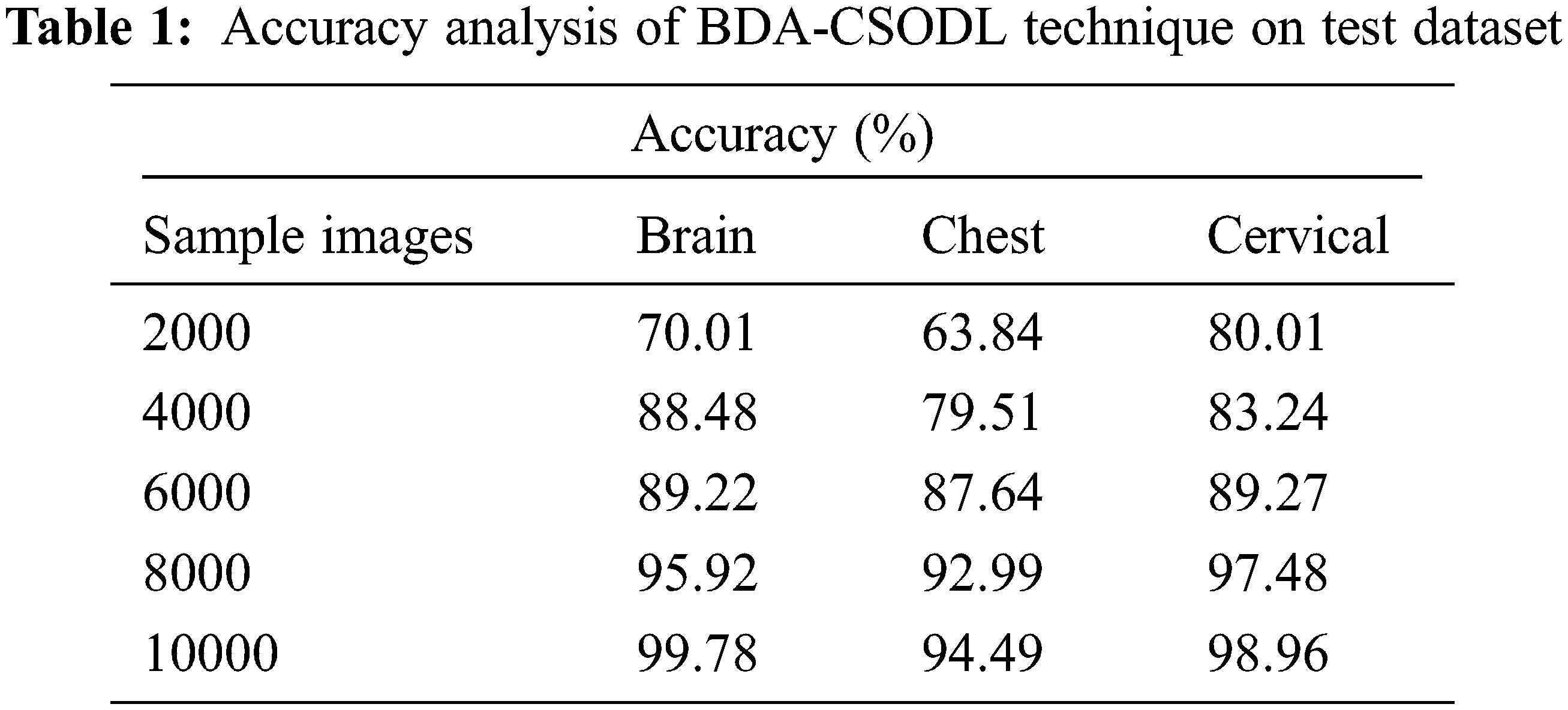
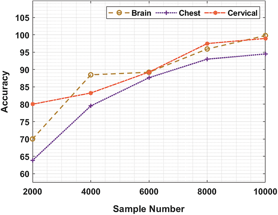
Figure 3: Result analysis of BDA-CSODL model in terms of accuracy

Tab. 2 and Fig. 4 showcase the results of kappa analysis accomplished by BDA-CSODL method on test dataset. The outcomes show that the proposed BDA-CSODL technique produced effective results with maximum kappa values on test samples. For instance, in case of 2,000 samples, BDA-CSODL approach reached kappa values such as 64.87%, 63.81%, and 74.71% on brain, chest, and cervical dataset correspondingly. Followed by, for 6,000 samples, BDA-CSODL methodology accomplished kappa values namely, 90.08%, 85.62%, and 87.86% on brain, chest, and cervical dataset correspondingly. However, in case of 10,000 samples, the proposed BDA-CSODL methodology attained kappa values such as 99.67%, 92.84%, and 98.85% on brain, chest, and cervical datasets correspondingly.

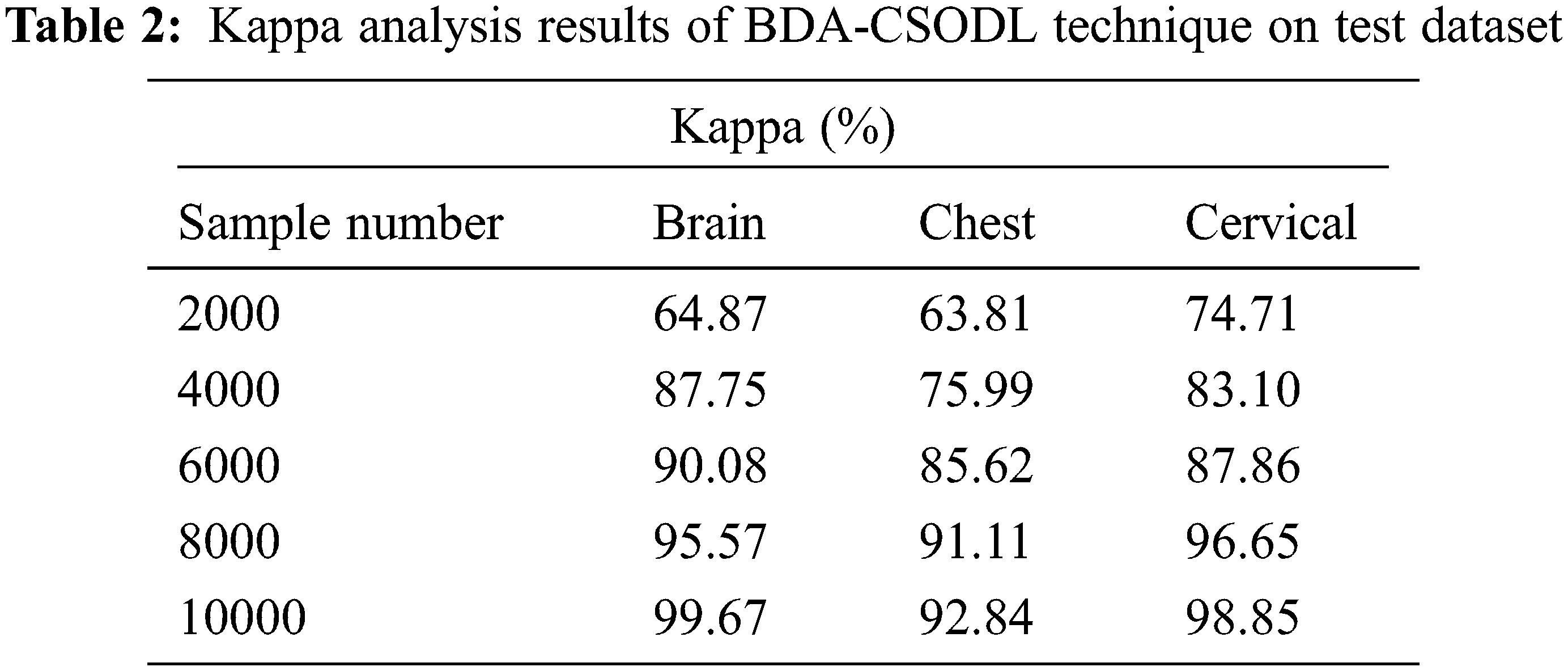
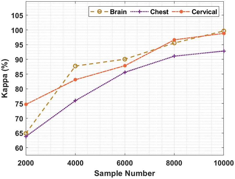
Figure 4: Analysis results of BDA-CSODL model in terms of kappa value

A brief comparison study was conducted between BDA-CSODL technique against existing approaches on brain dataset and the results are shown in Tab. 3 and Figs. 5–6. The results demonstrate that the proposed BDA-CSODL technique showcased better outcomes than other techniques in terms of accuracy and kappa under different images. With respect to accuracy, BDA-CSODL technique accomplished the maximum performance whereas CNNSVM, FR-CNN, and SVM techniques obtained minimum performance. For instance, with I-2000 samples, the proposed BDA-CSODL technique accomplished an effectual outcome with high accuracy of 0.700, whereas DL-GAN, DL-CNN, FR-CNN, CNNSVM, and SVM techniques obtained low accuracy values such as 0.695, 0.585, 0.547, 0.537, and 0.562 respectively. Additionally, with I-6000 samples, the proposed BDA-CSODL approach accomplished an effective outcome with superior accuracy of 0.892, whereas DL-GAN, DL-CNN, FR-CNN, CNNSVM, and SVM methodologies gained minimum accuracy values such as 0.889, 0.788, 0.863, 0.858, and 0.820 correspondingly. Besides, with I-10000 samples, the proposed BDA-CSODL method accomplished efficient outcomes with a high accuracy of 0.998, whereas other techniques such as DL-GAN, DL-CNN, FR-CNN, CNNSVM, and SVM produced less accuracy values such as 0.996, 0.988, 0.981, 0.884, and 0.975 correspondingly.

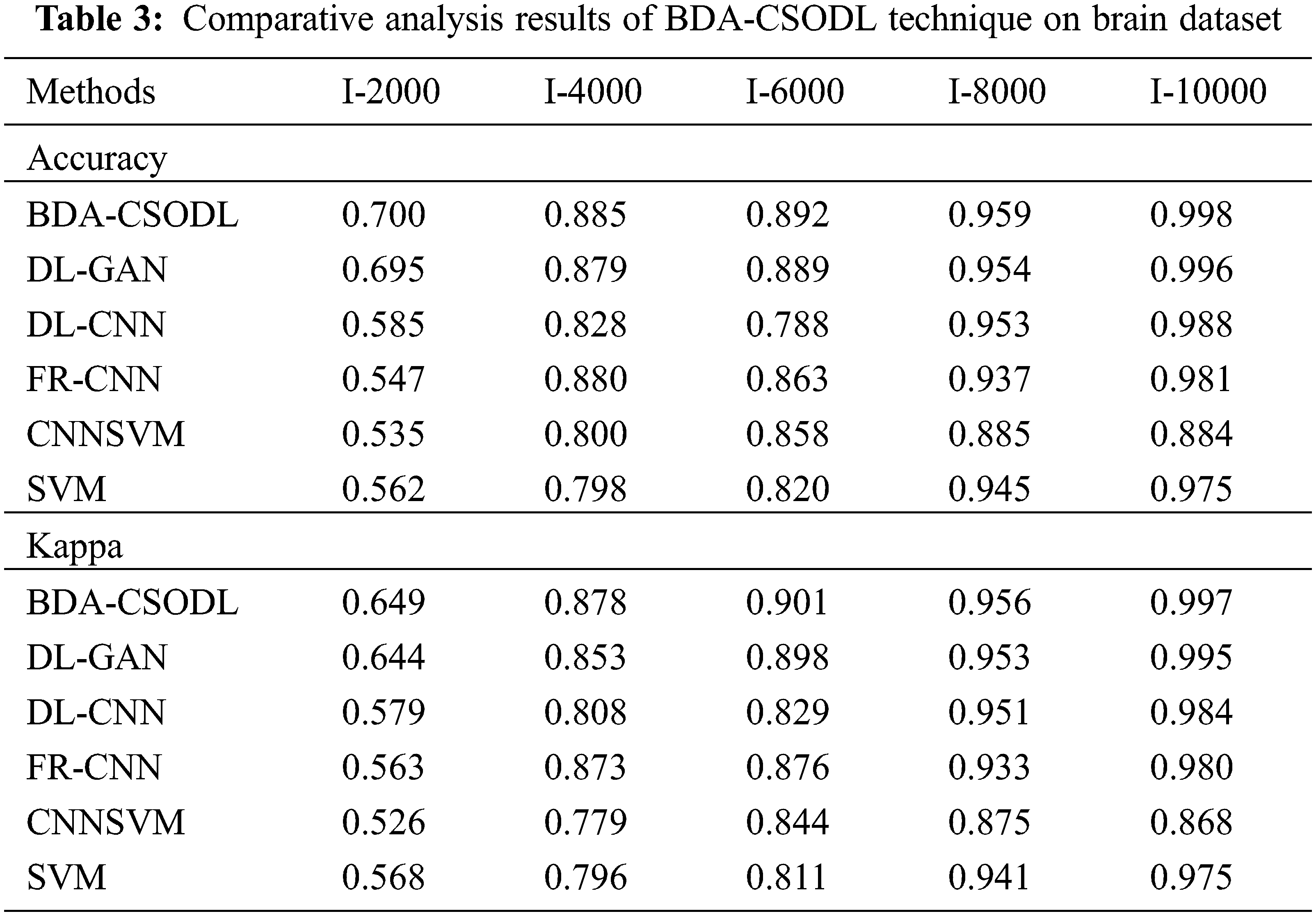
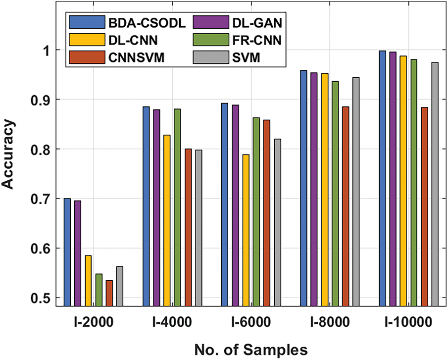
Figure 5: Accuracy analysis results of BDA-CSODL model on brain dataset

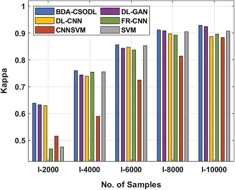
Figure 6: Kappa analysis results of BDA-CSODL model on brain dataset

With respect to kappa, the proposed BDA-CSODL algorithm accomplished the maximum performance, whereas CNNSVM, FR-CNN, and SVM methods gained the least performance. For instance, for I-2000 samples, BDA-CSODL method accomplished effectual results with a maximum kappa of 0.649, whereas DL-GAN, DL-CNN, FR-CNN, CNNSVM, and SVM methods achieved low kappa values such as 0.644, 0.579, 0.563, 0.526, and 0.568 respectively. In the meantime, with I-6000 samples, BDA-CSODL system accomplished an effective outcome with a high kappa value i.e., 0.901. However, DL-GAN, DL-CNN, FR-CNN, CNNSVM, and SVM approaches gained minimal kappa values namely, 0.898, 0.829, 0.876, 0.844, and 0.811. Eventually, with I-10000 samples, the proposed BDA-CSODL method accomplished an efficient outcome with high kappa of 0.997, whereas other techniques such as DL-GAN, DL-CNN, FR-CNN, CNNSVM, and SVM methods achieved minimum kappa values namely, 0.995, 0.984, 0.980, 0.868, and 0.975 correspondingly.

A detailed comparative analysis was conducted between BDA-CSODL approach and existing methods on chest dataset and the results are shown in Tab. 4. The outcomes showcase that the proposed BDA-CSODL algorithm produced excellent results than other methodologies with respect to accuracy and kappa in different samples.

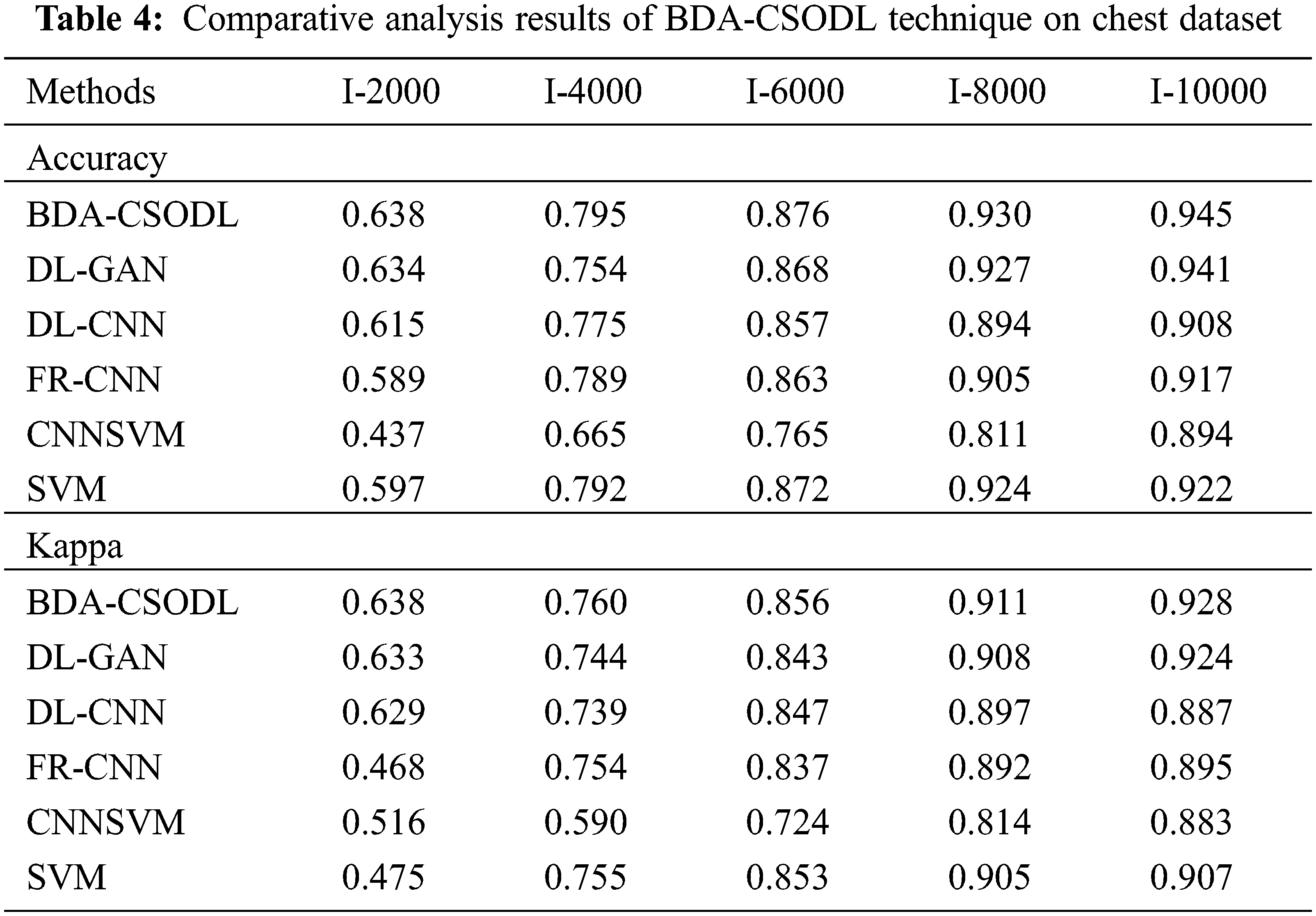
In terms of accuracy, the proposed BDA-CSODL method accomplished a high efficiency whereas CNNSVM, FR-CNN, and SVM methods gained low performance. For instance, with I-2000 samples, the proposed BDA-CSODL algorithm accomplished effectual results with a maximum accuracy of 0.638, whereas other techniques such as DL-GAN, DL-CNN, FR-CNN, CNNSVM, and SVM gained minimal accuracy values such as 0.634, 0.615, 0.589, 0.437, and 0.597 correspondingly. In addition, with I-6000 samples, BDA-CSODL algorithm accomplished effectual results with a high accuracy of 0.876, whereas DL-GAN, DL-CNN, FR-CNN, CNNSVM, and SVM systems obtained the least accuracy values such as 0.868, 0.857, 0.863, 0.765, and 0.872 correspondingly. Also, with I-10000 samples, the proposed BDA-CSODL technique accomplished an effectual outcome with a high accuracy of 0.945, whereas DL-GAN, DL-CNN, FR-CNN, CNNSVM, and SVM algorithms gained minimum accuracy values namely, 0.941, 0.908, 0.917, 0.894, and 0.922.

With respect to kappa, BDA-CSODL approach accomplished the maximal performance whereas other techniques such as CNNSVM, FR-CNN, and SVM achieved minimal performance. For instance, with I-2000 samples, the proposed BDA-CSODL system accomplished effective outcomes with an improved kappa of 0.638, whereas DL-GAN, DL-CNN, FR-CNN, CNNSVM, and SVM methods attained minimum kappa values namely, 0.633, 0.629, 0.468, 0.516, and 0.475 correspondingly. At the same time, with I-6000 samples, the proposed BDA-CSODL approach accomplished efficient outcomes with a high kappa of 0.856, whereas DL-GAN, DL-CNN, FR-CNN, CNNSVM, and SVM methods gained minimal kappa values namely, 0.843, 0.847, 0.837, 0.724, and 0.853. Finally, with I-10000 samples, the presented BDA-CSODL methodology accomplished efficient results with a high kappa of 0.928, whereas other techniques such as DL-GAN, DL-CNN, FR-CNN, CNNSVM, and SVM algorithms gained minimum kappa values such as 0.924, 0.887, 0.895, 0.883, and 0.907 correspondingly.

A brief comparative analysis was conducted between the proposed BDA-CSODL approach against recent algorithms on cervical dataset and the results are shown in Tab. 5. The results depict that the proposed BDA-CSODL methodology produces optimal results than other approaches with respect to accuracy and kappa under set of distinct images.

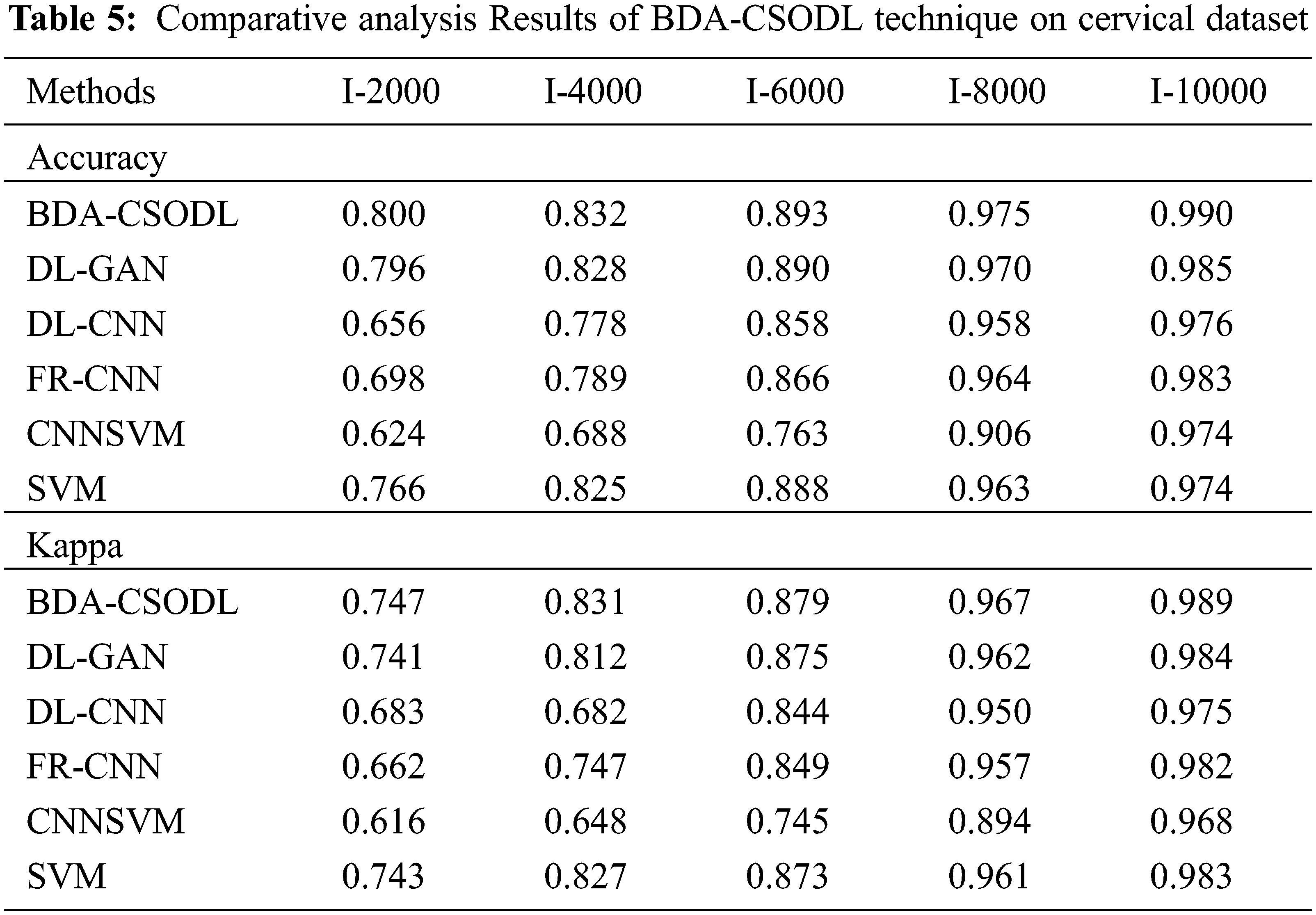
In terms of accuracy, the proposed BDA-CSODL methodology accomplished a maximal performance outcome whereas CNNSVM, FR-CNN, and SVM approaches gained minimal performance outcomes. For instance, with I-2000 samples, BDA-CSODL methodology accomplished an effective outcome with an increased accuracy of 0.800, whereas other techniques such as DL-GAN, DL-CNN, FR-CNN, CNNSVM, and SVM methods gained minimal accuracy values such as 0.796, 0.656, 0.698, 0.624, and 0.766 correspondingly. Along with that, for I-6000 samples, the proposed BDA-CSODL technique accomplished effective results with enhanced accuracy i.e., 0.893, whereas other techniques such as DL-GAN, DL-CNN, FR-CNN, CNNSVM, and SVM approaches achieved the least accuracy values such as 0.890, 0.858, 0.866, 0.763, and 0.888 correspondingly. Meanwhile, with I-10000 samples, the proposed BDA-CSODL system accomplished efficient outcomes with a superior accuracy of 0.990, whereas DL-GAN, DL-CNN, FR-CNN, CNNSVM, and SVM techniques attained minimum accuracy values namely, 0.985, 0.976, 0.983, 0.974, and 0.974.

In terms of kappa, the proposed BDA-CSODL approach accomplished a high efficiency, whereas CNNSVM, FR-CNN, and SVM methodologies gained the least efficiency values. For instance, with I-2000 samples, BDA-CSODL method accomplished effective results with an increased kappa of 0.747, whereas DL-GAN, DL-CNN, FR-CNN, CNNSVM, and SVM systems achieved minimum kappa such as 0.741, 0.683, 0.662, 0.616, and 0.743 correspondingly. Simultaneously, with I-6000 samples, the proposed BDA-CSODL approach accomplished an efficient outcome with a maximum kappa of 0.879, whereas DL-GAN, DL-CNN, FR-CNN, CNNSVM, and SVM techniques gained low kappa values namely, 0.875, 0.844, 0.849, 0.745, and 0.873. Concurrently, with I-10000 samples, the proposed BDA-CSODL method accomplished effectual outcomes with a superior kappa of 0.989. However, other techniques such as DL-GAN, DL-CNN, FR-CNN, CNNSVM, and SVM algorithms achieved low kappa values such as 0.984, 0.975, 0.982, 0.968, and 0.983 correspondingly. From the above discussed results, it is apparent that the proposed BDA-CSODL technique has accomplished effectual medical image classification performance.

5  Conclusion

In this study, a new BDA-CSODL technique is presented for biomedical image classification in Apache Spark environment. BDA-CSODL technique encompasses BF-based preprocessing, Otsu-based segmentation, Inception v3-based feature extraction, SGD-based hyperparameter optimization, LSTM-based classification, and CSO-based parameter tuning. Both SGD and CSO algorithms are designed in such a way that it considerably boosts medical image classification performance. In order to showcase the superior performance of BDA-CSODL approach, a comprehensive experimental analysis was carried out against benchmark medical images. The obtained experimental results showcase the supremacy of the proposed BDA-CSODL technique over other recent techniques under different performance measures. In future, multi-modal fusion-based medical image classification techniques can be designed to accomplish enhanced classification results.

Acknowledgement: The author extends his appreciation to the Deanship of Scientific Research at Majmaah University for funding this study under Project Number (R-2022-61).

Funding Statement: The authors received no specific funding for this study.

Conflicts of Interest: The authors declare that they have no conflicts of interest to report regarding the present study.

This work is licensed under a Creative Commons Attribution 4.0 International License, which permits unrestricted use, distribution, and reproduction in any medium, provided the original work is properly cited.