DOI:10.32604/csse.2023.026018
| Computer Systems Science & Engineering DOI:10.32604/csse.2023.026018 | |
| Article |
An Artificial Neural Network-Based Model for Effective Software Development Effort Estimation
1Department of Computer Science and Engineering, Kongju National University, Cheonan, 31080, Korea
2Department of Computer Science, COMSATS University Islamabad, Wah Campus, Islamabad, 47040, Pakistan
3Centre of AI and Data Science, Edinburgh Napier University, Edinburgh, EH11 4DY, UK
*Corresponding Author: Jungeun Kim. Email: jekim@kongju.ac.kr
Received: 13 December 2021; Accepted: 21 February 2022
Abstract: In project management, effective cost estimation is one of the most crucial activities to efficiently manage resources by predicting the required cost to fulfill a given task. However, finding the best estimation results in software development is challenging. Thus, accurate estimation of software development efforts is always a concern for many companies. In this paper, we proposed a novel software development effort estimation model based both on constructive cost model II (COCOMO II) and the artificial neural network (ANN). An artificial neural network enhances the COCOMO model, and the value of the baseline effort constant A is calibrated to use it in the proposed model equation. Three state-of-the-art publicly available datasets are used for experiments. The backpropagation feedforward procedure used a training set by iteratively processing and training a neural network. The proposed model is tested on the test set. The estimated effort is compared with the actual effort value. Experimental results show that the effort estimated by the proposed model is very close to the real effort, thus enhanced the reliability and improving the software effort estimation accuracy.
Keywords: Software cost estimation; neural network; backpropagation; forward neural networks; software effort estimation; artificial neural network
Effort estimation is the most critical activity in project management to efficiently manage resources through predicting the amount of effort required to perform a given task [1]. Accurate estimation, which influences software development management, increases the likelihood of completing software development tasks quickly and on budget. On the other hand, if the predictions are too low, it will put time pressure on the development team, resulting in residual errors due to incomplete software functionality and insufficient testing. Conversely, suppose the predictions are too high. In that case, it will cause an over-allocation of resources and development staff, which will make a company unable to obtain a contract due to uncompetitive contract offers. The proposed COCOMO II model used the COCOMO II 2000 calibrated post-architecture submodel with 5 SF and 17 EM with standard numerical values [2]. Neural networks are trained using previous data and automatically adjust algorithmic parameter values to reduce prediction errors. Most of the models that are developed using neural networks use backpropagation networks. ANN is encouraged by the characteristics of a biological neural network [3]. Each connecting link that connects one neuron to another is associated with weights. The weights have information about the input signals, and these weights are multiplied by their corresponding inputs to solve a particular problem.
Software project management is an essential activity in estimating the cost of software to perform a specific task. For this reason, studies have focused on presenting models for the relationship between the size and requirements of the software and its cost. However, the software effort estimating process still has gaps and problems, and the first phase of the project life cycle has not provided sufficient data. Finding the best cost estimation results is also a challenging task. The need for improved and accurate software effort estimation methods is a critical problem that software project management companies face.
In this paper, we proposed a novel software development effort estimation model. The proposed model will be a mixture of an algorithmic technique Constructive Cost Model II (COCOMO II) [4] and an artificial intelligence approach Neural Networks (NN). It will improve COCOMO II through ANN, helping project managers make estimates as accurate as possible for the successful execution of software projects. We have calibrated the value of baseline effort constant ‘A’ to use it in the proposed model equation. The proposed model is tested and trained on three publicly available datasets. The proposed model is also compared with the others state-of-the-art models. The backpropagation feedforward procedure is utilized with the iteratively processed training set (TS) for neural network training. Finally, the proposed model is tested on the testing set (VS).
The rest of the paper is organized as follows: Section 2 contains a literature review; Section 3 presents the proposed model, ca libration of constant ‘A’, model equation, and model architecture. Sections 4 and 5 describe the model algorithm and the details of the dataset. Section 6 discusses the data manipulations and the implementation of the model. Section 7 presents the results of the experiments and a discussion. Finally, Section 8 provides a model evaluation and compares the proposed model with other models, and Section 9 concludes the paper.
Several research studies are conducted to measure effort and cost estimation techniques [5–7]. Lawrence H. Putnam developed the Software Life Cycle Model (SLIM), also known as the Putnam model, and his original paper was published in 1978 [8]. To estimate the cost of the software, SLIM uses Source Lines of Code (SLOC). Putnam's life cycle analysis [9] serves as the basis for this model. Code size are the basic inputs for estimating software costs, and the output is effort [10–12]. Howard Rubin pioneered the use of ESTIMACS in the 1970s [13]. Initially developed as a Rapid Estimation System (QUEST), it was later combined with Management and Informatics Services (MACS) to form ESTIMACS. ESTIMACS is a proprietary model, so no internal details are available. Ricardo Valerdi [14] created the COSYSMO cost model for construction systems engineering in 2002. It is the most recent addition to the COCOMO family of cost estimation software models [15]. Barry Boehm and his USC students began work on COCOMO II research in 1994.
The Delphi technique is a well-known expert technique developed in the 1940s by the Rand Corporation as a forecasting method for predicting future events [16,17]. Planning poker estimates effort from expert judgment that was first defined by James Grenning in 2002. By combining the opinions of various experts, this technique generates an estimate of effort [18]. The origins of neural networks (NN) go back to the work of Warren McCulloch and Walter Pitts [19]. In 1979, Allan Albrecht developed the function points (FP) technique, which estimates working hours by counting the number of functions [20]. In 1993, Gustav Karner introduced the case point technique (UCP), which is based on principles similar to the FP estimation technique [21]. There are few studies found in the literature which also use COCOMO and neural networks. In [22] proposed a Neuro-Fuzzy COCOMO, which uses experts’ interpretation and allows input of linguistic values. The neural networks approaches are presented in [23–26]. They are different from our proposed model in many ways, such as the value of the baseline effort constant, the type of activation function used, and some other distinguishing features pointed out in Section 9.
3 Proposed Artificial Neural Network Model
The proposed model is a blend of COCOMO II and neural networks. The COCOMO model is improved by using the neural network approach. The subject model accommodates COCOMO II by using all of its Scale Factors and Effort Multipliers as an input to estimate the Effort.
3.1 Calibration of Constant ‘A’
The main problem of COCOMO II is time of development (TDEV) is not appropriate for small projects. The COCOMO II model is not well performed for small projects. In COCOMO II, most of the extensions are still experimental and have not been fully calibrated.
Eq. (1) of the COCOMO II is as follows:
In COCOMO II.2000, the default value of A is 2.94, but for the current scenario, the value of constant A is calibrated. For calibrating the constant A, at least 5 data points from the projects are recommended to use [2], so we have used 7 data points from NASA projects in the NASA 93 dataset for accurate estimation of results. Tab. 1 shows seven projects that have five attributes. In the first column (PMactual), the actual Effort of the projects in person months is listed. In the second column (EstimatesUnadjusted), the effort estimates are calculated against each corresponding project without using the value of constant A. In the third column ln(PMactual), natural logs (ln–log to the base e) of the actual effort are taken. In fourth column ln(EstimatesUnadjusted), natural logs of the unadjusted estimates is taken. Finally, the difference between ln(PMactual) and ln(EstimatesUnadjusted) is determined in the fifth column.
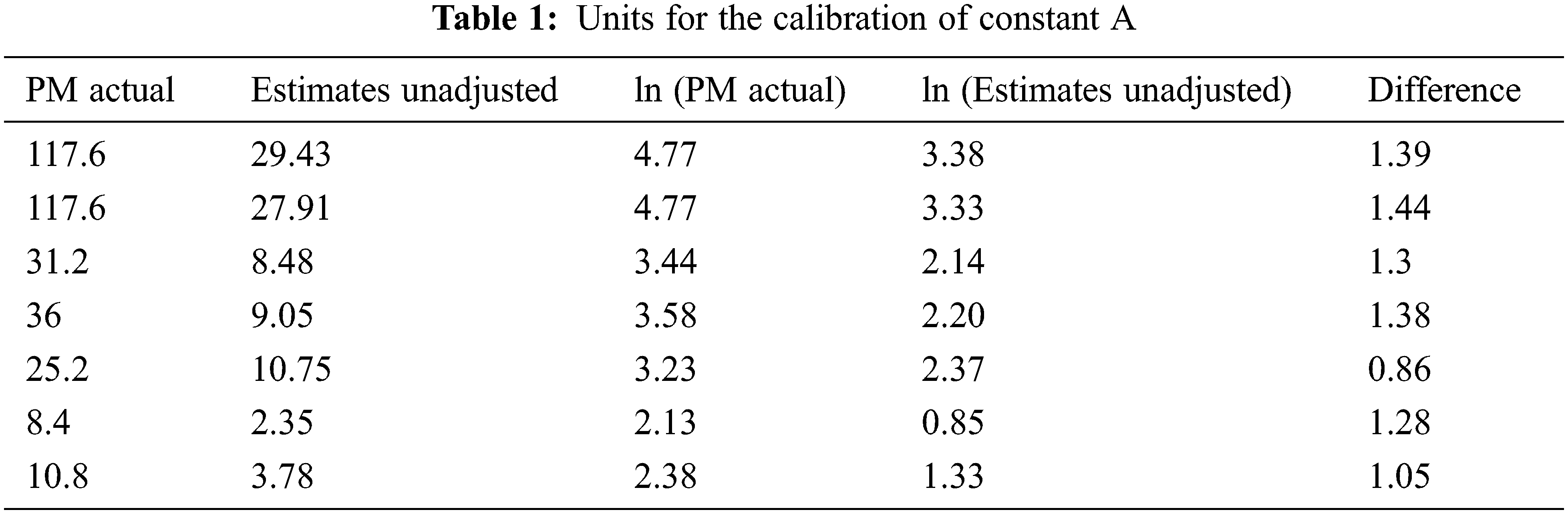
After that, the average of the differences is obtained by:
And finally, the constant A is determined after calculating the anti-log (ex) of average of differences by:
After rounding off the figure, we get the value of 3.47. Hence, instead of using A = 2.94, a locally calibrated constant A = 3.47 is used in the proposed model.
The proposed model accommodates the equation of the COCOMO II model in exponential form, so the natural log (ln) is taken on both sides of Eq. (1) to convert it into linear form. The equation is simplified as stated below:
If we ignore the constants, i.e., ln(A) and value of B, which is 0.91, from the above equation and use them as biases in the neural network, the result is Eq. (2).
The parameters in equation two will be given as inputs to the neural network. Thus, the resulting Eq. (3) is shown below:
where,
WEM1 to WEM17 weights for I1 to I17 and WSF18 + ln (size) to WSF22 + ln (size) weights for I18 to I22. So, here we have the generic Eqs. (4)–(6).
WP and Wq are the weights for CEM and CSF.
The proposed model will get a total of 24 inputs. The neural network model will accommodate COCOMO II to use all of its parameters as an input. There are two biases17 EMs, and 5 SFs. Fig. 1 shows the first part of the proposed model.
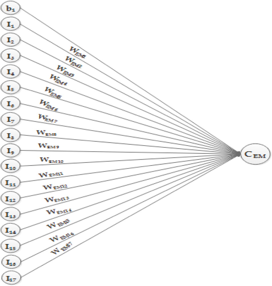
Figure 1: Inputs for CEM
It shows that there are 18 inputs, I1 to I17 and one bias in the input layer, which will contribute to obtaining the value of CEM in the hidden layer. All of these inputs are preprocessed. EMs are given as input after taking the natural log – ln (log to the base e) and bias b1 is assigned the value of multiplicative constant A after taking its natural log ln(A). WEM1 to WEM17 are the weights associated with each connection link. Now, the second part of the proposed model is presented in Fig. 2.
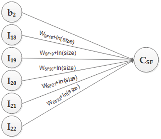
Figure 2: Inputs for CSF
Fig. 2 shows six inputs, I18 to I22 and one bias, which will contribute to obtaining the value of CSF in the hidden layer. All of these inputs are preprocessed. SFs is given as input after multiplying by 0.01, and bias b2 is given the value of B, which is 0.91. The weights associated with each connection link are WSF18 + ln (size) to WSF22 + ln (size). The size is taken to determine the very initial weights of the SFs. Now, the third portion of the proposed model is shown. Fig. 3 shows two neurons in the hidden layer CEM and CSF, providing input signals to the output layer CPM. CEM and CSF will contribute to getting the value of CPM in the output layer. WP and Wq are the weights associated with each connection link. CPM will provide effort as an output in the form of ln(PM) and ln of effort in person-months. The generic architecture is depicted in Fig. 4, through which the complete picture of the proposed model is shown
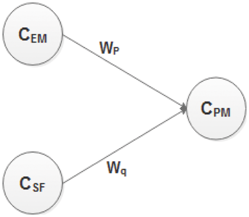
Figure 3: Inputs for CPM
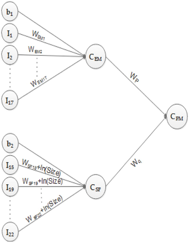
Figure 4: The generic architecture of the proposed model
4 Proposed Artificial Neural Network Model Algorithm
This section provides an algorithm for training neural networks. The backpropagation feedforward procedure is employed for this purpose. The algorithm for training, computing weights for the proposed network, and testing is as follows:
i) Initialize a network.
ii) Assign initial values to weights: WEM = 1, WSF = 0, WP = 1, Wq= 1.
iii) Assign values to biases: b1 = 1.244154594, b2 = 0.91
iv) Set Learning Rate: l_rate = 0.1
v) Set the activations for the input units: Ii = TSj where i = 1 to 22, TS is the training set, and j is the jth data-point.
vi) CEM and CSF calculate the net input by summing up their weighted input signals.
vii) Apply the sigmoid activation function in CEM and CSF. The sigmoid function is defined as
viii) Multiply the output of the two hidden layer neurons with their weights and calculate the weighted sum to obtain CPM.
ix) These are forward propagation steps. Now do the following steps of backpropagation in which error correction terms will be calculated, and then weights will be changed.
x) Calculate error correction term at CPM, CEM, and CSF:
xi) Update the weights for the hidden laer:
xii) Update weights for input layer:
xiii) Update biases:
xiv) These are the training steps; run the training step using two nested loops. The outer loop will iterate 140 times, which is the number of data points in TS. The inner loop will iterate 100 times to adjust the weights according to the actual output.
xv) When training is done, the latest updated weights will be used to test the network.
xvi) Test the network over 28 data points in Testing Set (VS).
Three publicly available datasets are used to test and train the proposed model. These three datasets are NASA 93 dataset, COCOMO 81 dataset, and COCOMO SDR dataset. These data sets are taken from the tera-PROMISE repository [27], an update to the older PROMISE repository for software engineering data.
The NASA 93 dataset contains 93 different NASA projects. This dataset initially has 26 attributes, but it is refined for the current scenario. After refinement, it contains a total of 24 attributes: 5 SFs and 17 EMs in 6 categories: very low (vl), low (l), nominal (n), high (h), very high (vh), extra high (xh); software size, and the actual effort.
The COCOMO 81 dataset contains 63 projects and 26 attributes and is refined for the current scenario. After refinement, it contains 24 attributes: 5 scale factors, 17 cost drivers, size (KDSI), and actual effort.
COCOMO SDR dataset contains 12 projects. This dataset initially has 24 attributes which are taken as it is in the current scenario. The attributes are 5 SFs, 17 EMs, size, and actual effort.
The dataset is split into 83 and 17; the 83% for network training and the remaining 17% to test the proposed network.
6 Dataset Manipulation and Model Implementation
Three publicly available datasets NASA 93, COCOMO 81, and COCOMO SDR, are used. The data of 93 projects, 63 projects, and 12 projects, respectively. These projects are merged into a single Comma-Separated Values file (CSV) consisting of 168 data points.
In the validation, two sets of inputs, EM and SF, are given to the model. EMs is given as input after taking the natural log – ln (log to the base e) and bias b1 is assigned the value of multiplicative constant A after taking its natural log, ln(A). SFs are given as input after multiplying by 0.01, and bias b2 is assigned the value of B, 0.91. The natural log of columns ‘Size’ and ‘Effort’ is also taken. After that, the dataset is divided into Training Set (TS) and Testing Set (VS), with 80% and 20% ratios to get more prediction accuracy. Then, the first 28 rows are used for testing the model, and last, the 140 records are used for model training. The model is implemented through Python programming language [28–30] – version Python 3.6.0 with the open data science platform Anaconda [31] - version 4.3.1. For coding, an open-source web application Jupyter Notebook [32], is used, which is an interactive computational environment. The implementation is done on Microsoft Windows 7 with a 64-bit operating system. The structure of the coding is based on the object-oriented programming paradigm (OOP) [33,34].
7 Experimental Results and Discussion
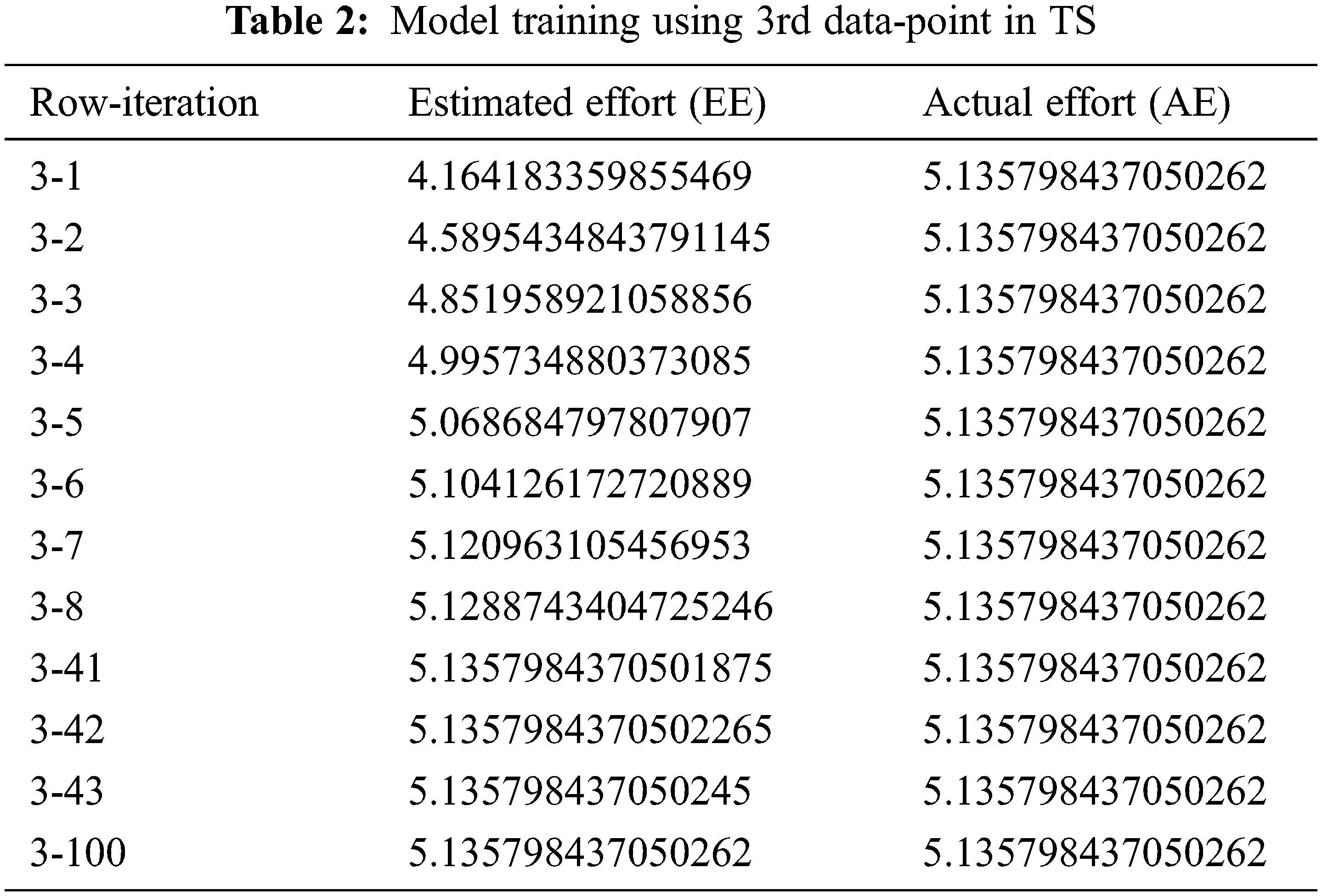
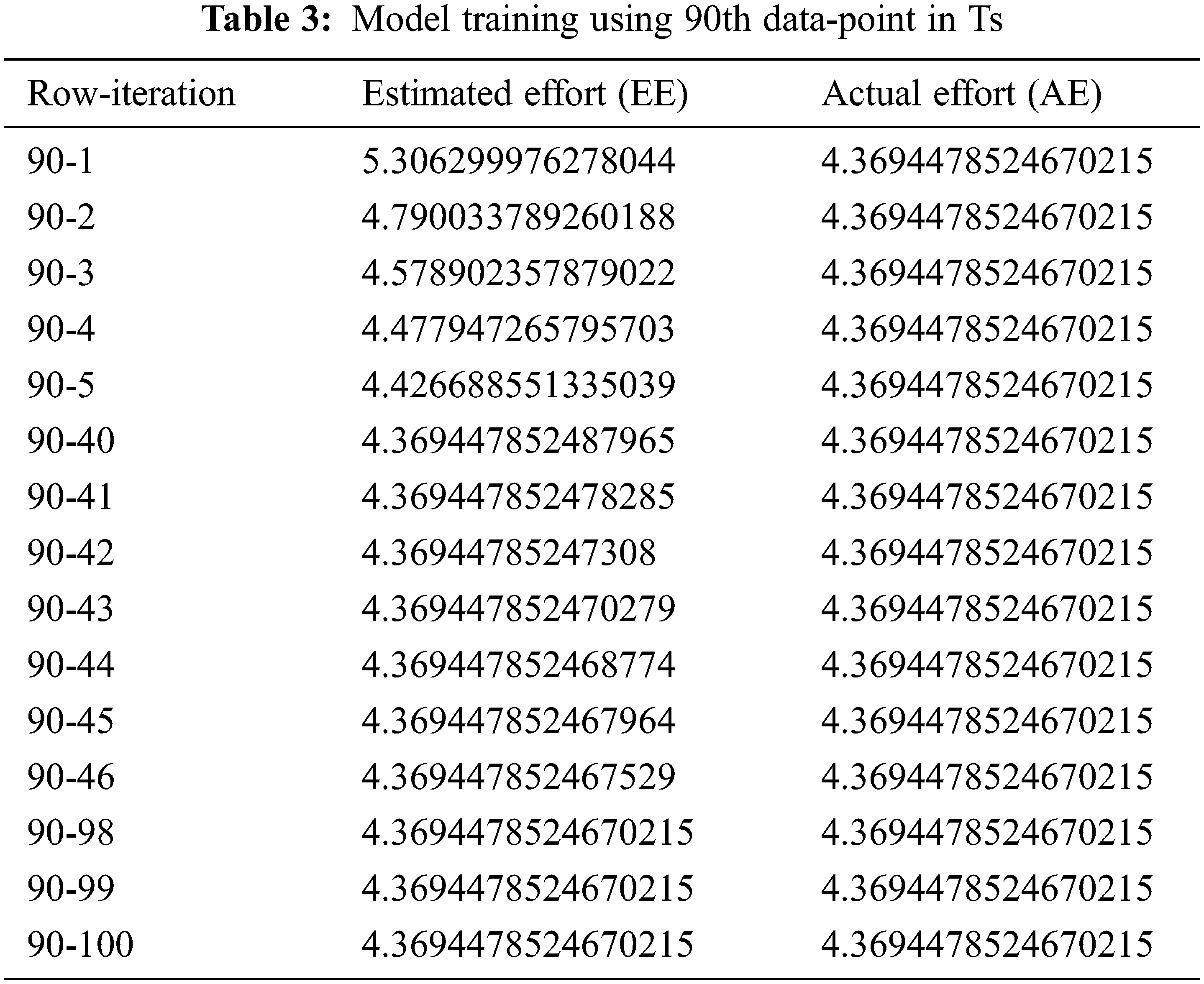
The backpropagation feedforward procedure is used for neural network training. First, training samples Training Set (TS) is processed iteratively to predict the Effort. There are 140 data points in TS and each data point/row is iterated 100 times. The estimated effort (EE) is then compared with the actual effort (AE) value. The error correction term is computed by taking the difference of AE and EE, and then the weights are modified. The weights for each training sample are updated to minimize the difference between EE and the AE. Tabs. 2 and 3 describe how supervised learning is performed on the network. After adjusting its weights, it tries to be close to the actual project effort (only two rows that are row 3 and row 90, with all of their 100 iterations are given as an example).
The proposed model is tested over the Test Set (VS), consisting of 17% of the dataset. There are 28 data points and data for 28 different projects in the testing set. After its training, the proposed model is tested in the testing set. It predicted the effort for the projects. Fig. 5 shows the results of the estimated effort (EE) for software development and the comparison of the actual effort (AE). The EE is very close to the AE, which validates the correctness of the proposed model. The comparison of the estimated effort and the actual effort shows that the proposed model worked well.
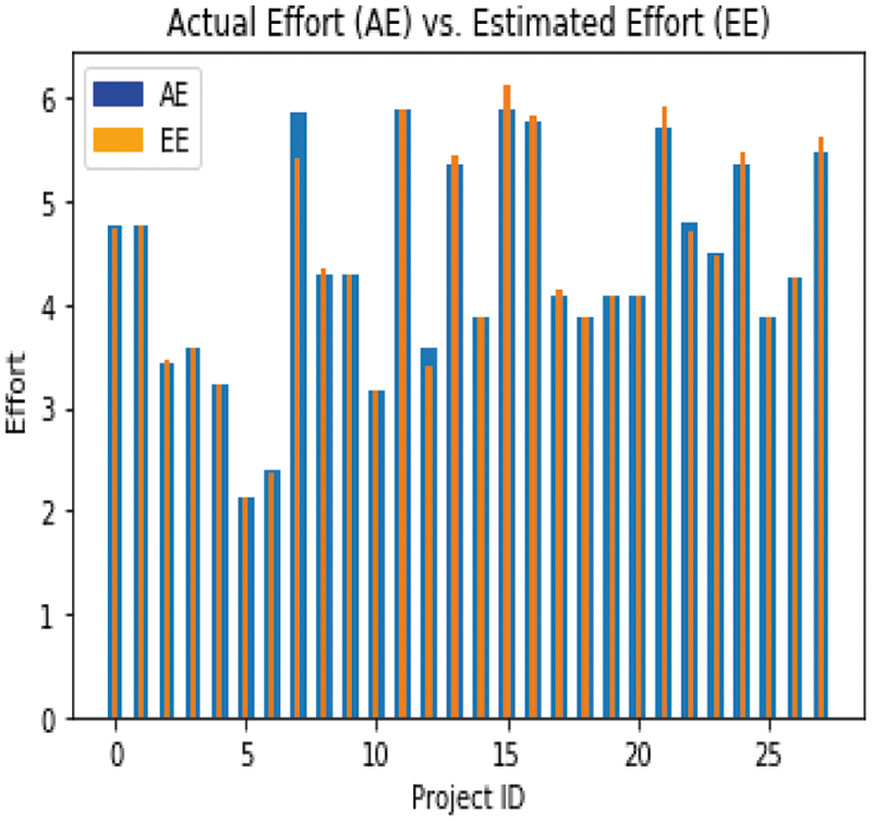
Figure 5: Comparison of AE vs. EE on the VS-bar chart
8 Model Evaluation and Comparison
Model evaluation means comparing the correctness of effort predicted by the proposed model with the actual effort. The proposed model is assessed by the most common and widely accepted evaluation criteria MRE and MMRE [35]. The MRE equation is below:
In the above equation, actual effort is taken from the dataset. The estimated effort is predicted by the proposed model and
The MMRE is defined as follows:
In the above equation, N is 28 - the data points for which the MRE is calculated. Thus, MMRE provides the average of MRE over N data points.
Fig. 6 illustrate the comparison of EE and AE with a bar chart. Therefore, it represents that the proposed model gives improved results than COCOMO II. The results shows that proposed model is more efficient than the COCOMO II model.
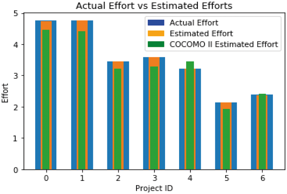
Figure 6: AE vs. Effort estimated by the proposed model and COCOMO-II-bar chart
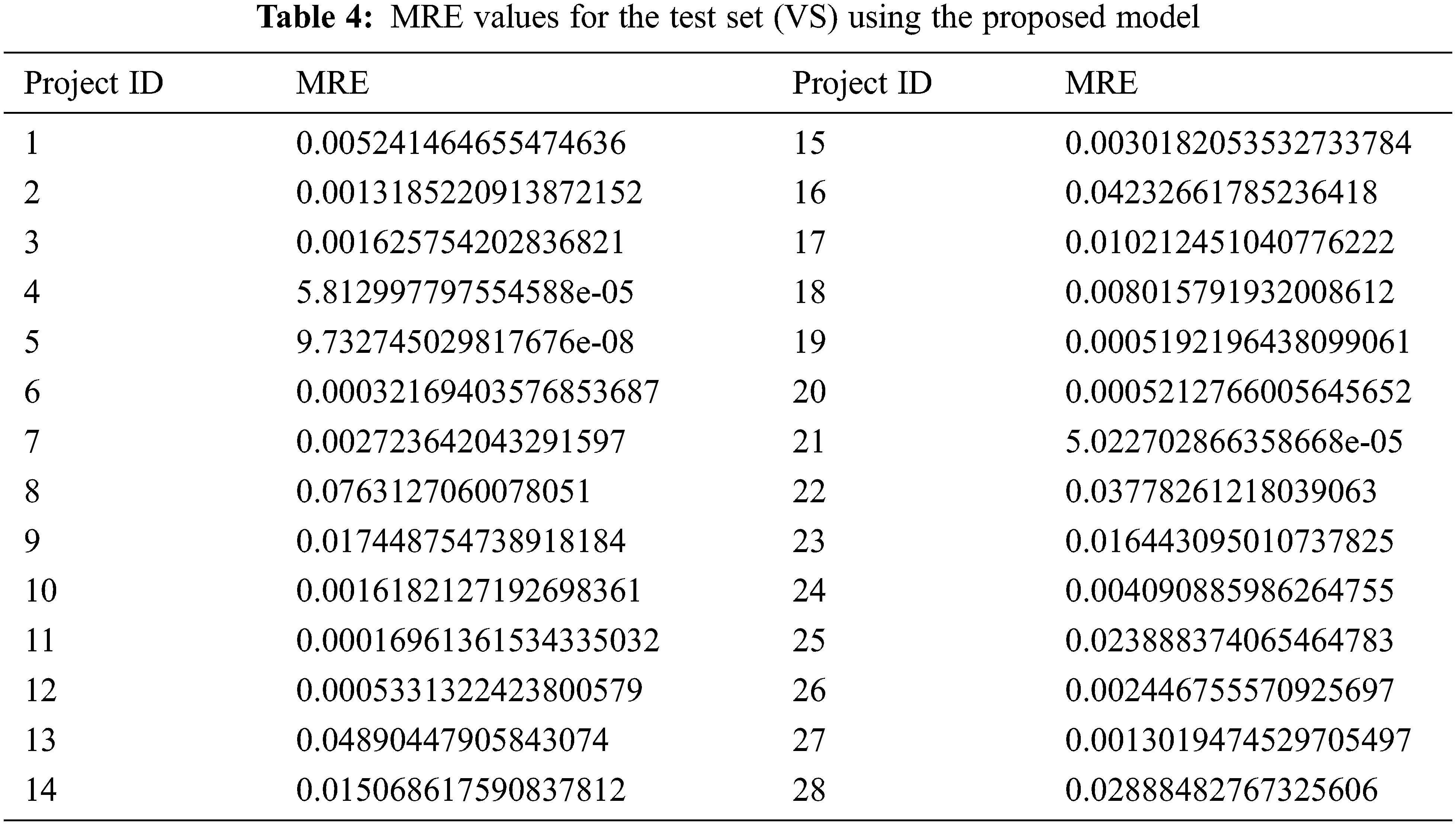
The MRE of the first 7 data points is calculated separately for the proposed model with COCOMO II. Fig. 7 illustrates the comparison of MRE values for the first 7 data points in the Testing Set (VS) for both the proposed model and COCOMO II. The lower the MRE, the better the results. The proposed model results are better than COCOMO II. Therefore, proposed model is better and more efficient than the COCOMO II.
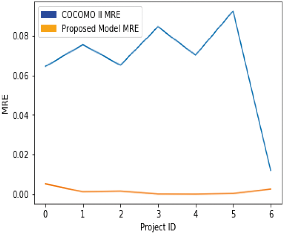
Figure 7: Comparison of MRE values using the proposed model and COCOMO-II grafh
The MMRE for the proposed model is 0.002, which is less than the MMRE for the COCOMO II model, which is 0.066, so it can be said that the proposed model gives better results than COCOMO II because the lower the MMRE, the better the predictions.
There are few studies found in the literature that used Neuro-Fuzzy COCOMO, NN for cost estimation [36,37] and cost estimation for web projects [38,39]. Fig. 8 shows MMRE results compared to other state-of-the-art models on the COCOMO 81 dataset. The results are also compared with neural network techniques. The significance of the BRE [40] values is shown to be massive for RBNN [41] and BPNN [42], even when the predicted and real values are small. The proposed model MMRE value is the smallest compared to previous state-of-the-art models BPNN, RBNN, COCOMO, and DANN [43]. The lowest MMRE indicates that proposed model estimation is better as compared to other models. Therefore, results indicated that the proposed model is more efficient than the others RBNN, BPNN, COCOMO and DANN.
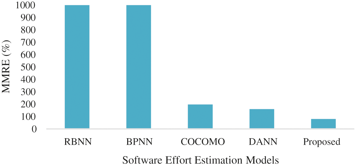
Figure 8: Comparison of MMRE values with other models
The distinguishing features of the proposed model as compared to others are given below.
• It uses COCOMO II.2000 calibrated values for Post-Architecture SFs and EMs.
• Its baseline effort constants and baseline schedule constants are A = 2.94, B = 0.91 and C = 3.67, D = 0.28, respectively.
• It uses the sigmoid function only in the hidden layer.
• It preprocesses the values of EMs and SFs by taking the natural log of EMs and multiplying SFs by 0.01 before using them as inputs.
• It calibrated the value of constant A (which is originally 2.94, and after calibration, it became 3.47) because calibration is an essential task that needs to be done to obtain an accurate estimation.
• Dataset is divided into the ratio of 83:17 for training and testing.
• It uses bias-1 and bias-2 as b1 = 1.244154594 and b2 = 0.91 respectively.
• The proposed model has the ability to learn and a fixed number of EM and SF parameters that need to be learned.
Effort estimation is the most critical activity in project management to manage resources efficiently by predicting the required amount of Effort to fulfill a given task. In this paper, we proposed a novel software development effort estimation model, designed using the COCOMO post-architecture model and artificial neural network (ANN). A prevalent and most widely used COCOMO model is enhanced by using the Neural Networks approach. We have calibrated the value of baseline effort constant A to use it in the model equation. Three publicly available datasets are used for testing and training the model. The backpropagation feedforward procedure is used by iteratively processing a set of training samples to train the network. After that, the proposed model is tested over the Testing Set (VS), and the estimated Effort is compared with the actual effort value. The experimental results show that the effort estimated by the proposed model is significantly closer to the actual effort than the COCOMO model and enhances the reliability with an improvement in software development effort estimation accuracy. The MMRE results indicate that the proposed model is better than COCOMO, BPNN, RBNN and DANN. Overall, the experimental results show that the proposed model outperforms for software effort estimation compared to other models.
In the future, we will improve the accuracy of the proposed model to provide a more accurate estimate of effort with some other machine learning approaches. We will also test the proposed model in various other software projects.
Funding Statement: This work was supported by the Technology development Program of MSS [No. S3033853].
Conflicts of Interest: The authors declare that they have no conflicts of interest to report regarding the present study.
1. M. Ruhe, R. Jeffery and I. Wieczorek, “Cost estimation for web applications,” in 25th Int. Conf. on Software Engineering, Portland, USA, pp. 285–294, 2003. [Google Scholar]
2. B. W. Boehm, “COCOMO II overview,” in 14th Int. COCOMO Forum, Los Angeles, USA, pp. 1–20, 1999. [Google Scholar]
3. A. K. Jain, J. Mao and K. M. Mohiuddin, “Artificial neural networks: A tutorial,” Computer, vol. 29, no. 3, pp. 31–44, 1996. [Google Scholar]
4. B. Boehm, B. Clark, E. Horowitz, C. Westland, R. Madachy et al., “Cost models for future software life cycle processes: COCOMO 2.0,” Annals of Software Engineering, vol. 1, no. 12, pp. 57–94, 1995. [Google Scholar]
5. B. Boehm, C. Abts and S. Chulani, “Software development cost estimation approaches—a survey,” Annals of Software Engineering, vol. 10, no. 1, pp. 177–205, 2000. [Google Scholar]
6. M. Jorgensen and M. Shepperd, “A systematic review of software development cost estimation studies,” IEEE Transactions on Software Engineering, vol. 22, no. 1, pp. 33–53, 2006. [Google Scholar]
7. J. Wen, S. Li, Z. Li, Y. Hu and C. Huang, “Systematic literature review of machine learning based software development effort estimation models,” Information and Software Technology, vol. 51, no. 1, pp. 41–59, 2021. [Google Scholar]
8. L. H. Putnam, “A general empirical solution to the macro software sizing and estimating problem,” IEEE Transactions on Software Engineering, vol. 4, no. 7, pp. 345–361, 1978. [Google Scholar]
9. B. W. Boehm, “Software engineering economics,” IEEE Transactions on Software Engineering, vol. 10, no. 1, pp. 4–21, 1984. [Google Scholar]
10. S. Kumari and S. Pushkar, “Comparison and analysis of different software cost estimation methods,” International Journal of Advanced Computer Science and Application, vol. 4, no. 1, pp. 153–157, 2013. [Google Scholar]
11. A. Arifoglu, “A methodology for software cost estimation,” ACM SIGSOFT Software Engineering Notes, vol. 18, no. 2, pp. 96–105, 1993. [Google Scholar]
12. F. J. Heemstra, “Software cost estimation. Information and software technology,” Applied Software Measurement, vol. 34, no. 10, pp. 627–639, 1992. [Google Scholar]
13. H. A. Rubin, “Macro-estimation of software development parameters: the estimacs system,” in SOFTFAIR Conf. on Software Development Tools, Techniques and Alternatives, Washington DC, USA, pp. 109–118, 1983. [Google Scholar]
14. R. Valerdi, “The constructive systems engineering cost model (COSYSMO),” Ph.D. dissertation, University of Southern California, USA, 2005. [Google Scholar]
15. V. K. Yadav, “Software cost estimation: Process, methods and tools,” Global Sci-Tech, vol. 9, no. 3, pp. 138–147, 2017. [Google Scholar]
16. N. Dalkey and O. Helmer, “An experimental application of the DELPHI method to the use of experts,” Management Science, vol. 9, no. 3, pp. 458–467, 1963. [Google Scholar]
17. R. Balasubramanian and A. Deepti, “Delphi technique--a review,” International Journal of Public Health Dentistry, vol. 3, no. 2, pp. 26, 2012. [Google Scholar]
18. K. Molokken-Ostvold and N. C. Haugen, “Combining estimates with planning poker--an empirical study,” in 2007 Australian Software Engineering Conf., Melbourne, Australia, pp. 349–358, 2007. [Google Scholar]
19. W. S. Mcuulloch and W. Pitts, “A logical calculus of the ideas immanent in nervous activity,” The Bulletin of Mathematical Biophysics, vol. 5, no. 4, pp. 115–133, 1943. [Google Scholar]
20. A. J. Albrecht and J. E. Gaffney, “Software function, source lines of code, and development effort prediction: A software science validation,” IEEE Transactions on Software Engineering, vol. 9, no. 6, pp. 639–648, 1983. [Google Scholar]
21. R. K. Clemmons, “Project estimation with use case points,” The Journal of Defense Software Engineering, vol. 19, no. 2, pp. 18–22, 2006. [Google Scholar]
22. X. Huang, D. Ho, J. Ren and L. F. Capretz, “Improving the COCOMO model using a neuro-fuzzy approach,” Applied Soft Computing, vol. 7, no. 1, pp. 29–40, 2007. [Google Scholar]
23. O. M. Tailor, A. M. Kumar and M. P. Rijwani, “A new high performance neural network model for software effort estimation,” International Journal of Innovative Science, Engineering & Technology, vol. 1, no. 3, pp. 400–405, 2014. [Google Scholar]
24. N. Tadayon, “Neural network approach for software cost estimation,” in Int. Conf. on Information Technology: Coding and Computing (ITCC’05), Las Vegas, USA, pp. 815–818, 2005. [Google Scholar]
25. A. Kaushik, A. K. Soni and R. Soni, “A simple neural network approach to software cost estimation,” Global Journal of Computer Science and Technology, vol. 13, no. 1, pp. 23–30, 1969. [Google Scholar]
26. I. Attarzadeh, “Proposing a new software cost estimation model based on artificial neural networks,” in 2010 2nd Int. Conf. on Computer Engineering and Technology, Chengdu, China, pp. 487–491, 2010. [Google Scholar]
27. Repository for SE Research Data. http://openscience.us/repo/. [Google Scholar]
28. G. Van, “Python programming language,” in USENIX Annual Technical Conf., Santa Clara, USA, pp. 1–36, 2007. [Google Scholar]
29. W. Chun, “Welcome to python,” in Core Python Programming, 1st ed., vol. 1. Hoboken, USA: Prentice Hall, pp. 1–23, 2001. [Google Scholar]
30. M. Lutz, “System tools,” in Programming Python: Powerful Object-Oriented Programming, 1st ed., vol. 1. Bejing, China: Reilly Media, pp. 73–100, 2010. [Google Scholar]
31. Open data science platform, Anaconda. https://www.anaconda.com/. [Google Scholar]
32. IPython Interactive Computing, The Jupyter Notebook. https://ipython.org/notebook.html. [Google Scholar]
33. P. Wegner, “Concepts and paradigms of object-oriented programming,” ACM Sigplan Oops Messenger, vol. 1, no. 1, pp. 7–87, 1990. [Google Scholar]
34. B. Stroustrup, “What is object-oriented programming?,” IEEE Software, vol. 5, no. 3, pp. 10–20, 1988. [Google Scholar]
35. M. Shepperd and S. MacDonell, “Evaluating prediction systems in software project estimation,” Information and Software Technology, vol. 54, no. 8, pp. 820–827, 2012. [Google Scholar]
36. J. Rashid and M. W. Nisar, “How to improve a software quality assurance in software development-a survey,” International Journal of Computer Science and Information Security, vol. 14, no. 8, pp. 99–108, 2016. [Google Scholar]
37. N. Rankovic, D. Rankovic, M. Ivanovic and L. Lazic, “A new approach to software effort estimation using different artificial neural network architectures and taguchi orthogonal arrays,” IEEE Access, vol. 9, no. 2, pp. 26926–26936, 2021. [Google Scholar]
38. S. Fedushko, T. Perace, Y. Syerov and O. Trach, “Development of methods for the strategic management of web projects,” Sustainability, vol. 12, no. 2, pp. 1–18, 2021. [Google Scholar]
39. D. K. Saini, “Fuzzy and mathematical effort estimation models for web applications,” Applied Computing Journal, vol. 1, no. 1, pp. 10–24, 2021. [Google Scholar]
40. S. Bilgaiyan, S. Sagnika, S. Mishra and M. Das, “A systematic review on software cost estimation in agile software development,” Journal of Engineering Science and Technology Review, vol. 10, no. 4, pp. 51–64, 2017. [Google Scholar]
41. N. Karunanithi, D. Whitley and Y. K. Malaiya, “Using neural networks in reliability prediction,” IEEE Software, vol. 9, no. 4, pp. 53–59, 1992. [Google Scholar]
42. M. Buscema, “Artificial neural networks and complex social systems models,” Substance Use and Misuse, vol. 33, no. 2, pp. 233–270, 1988. [Google Scholar]
43. N. K. Alhammad, E. Alzaghoul, F. A. Alzaghoul and M. Akour, “Evolutionary neural network classifiers for software effort estimation,” International Journal of Computer Aided Engineering and Technology, vol. 12, no. 4, pp. 495–512, 2020. [Google Scholar]
 | This work is licensed under a Creative Commons Attribution 4.0 International License, which permits unrestricted use, distribution, and reproduction in any medium, provided the original work is properly cited. |