DOI:10.32604/csse.2023.026128
| Computer Systems Science & Engineering DOI:10.32604/csse.2023.026128 | |
| Article |
Deep Learning with Optimal Hierarchical Spiking Neural Network for Medical Image Classification
1Department of Computer Science and Engineering, Anjalai Ammal Mahalingam Engineering College, Koilvenni, 614403, Tamil Nadu, India
2Department of CSE, E.G.S. Pillay Engineering College, Nagapattinam, 611002, Tamil Nadu, India
*Corresponding Author: P. Immaculate Rexi Jenifer. Email: irexijp@gmail.com
Received: 16 December 2021; Accepted: 24 January 2022
Abstract: Medical image classification becomes a vital part of the design of computer aided diagnosis (CAD) models. The conventional CAD models are majorly dependent upon the shapes, colors, and/or textures that are problem oriented and exhibited complementary in medical images. The recently developed deep learning (DL) approaches pave an efficient method of constructing dedicated models for classification problems. But the maximum resolution of medical images and small datasets, DL models are facing the issues of increased computation cost. In this aspect, this paper presents a deep convolutional neural network with hierarchical spiking neural network (DCNN-HSNN) for medical image classification. The proposed DCNN-HSNN technique aims to detect and classify the existence of diseases using medical images. In addition, region growing segmentation technique is involved to determine the infected regions in the medical image. Moreover, NADAM optimizer with DCNN based Capsule Network (CapsNet) approach is used for feature extraction and derived a collection of feature vectors. Furthermore, the shark smell optimization algorithm (SSA) based HSNN approach is utilized for classification process. In order to validate the better performance of the DCNN-HSNN technique, a wide range of simulations take place against HIS2828 and ISIC2017 datasets. The experimental results highlighted the effectiveness of the DCNN-HSNN technique over the recent techniques interms of different measures. Please type your abstract here.
Keywords: Medical image classification; spiking neural networks; computer aided diagnosis; medical imaging; parameter optimization; deep learning
With the growing demands for more accurate and faster treatment, medical imaging play a significant part in the earlier diagnosis, treatment, and detection of diseases [1]. Due to the growth of computer science and technology, physics, and electronic engineering, the solution of medical images are increasingly high, and the image modes are increasingly abundant. Simultaneously, the number of medical images is rapidly increasing. Now, positron emission tomography (PET/CT), ultrasound imaging, computed tomography (CT), magnetic resonance imaging (MRI), X-ray imaging, are used extensively in hospitals. The key to attaining an appropriate treatment and diagnosis is the appropriate interpretation of medical image, however, interpretation of the image is based largely on the subjective decision of physicians, and hence physicians at distinct stages have considerable deviance on the outcomes of image interpretation [2]. Recently, with the development of a huge amount of labeled natural image datasets and the advance of deep learning in image classification, image segmentation, computer vision, and target detection have been improved considerably. Numerous studies were conducted on earlier diagnosis and detection of diseases according to the supervised learning model.
Medical image classification has become one of the major problems in the image recognition field and aims to categorize medical images into different kinds to assist physicians in additional studies/disease diagnoses [3]. Generally, medical image classification could be separated into 2 phases. Initially, extract efficient features from the image. Next, utilizing the feature to construct models which categorize the image datasets. Earlier, physicians widely employed their professional skill for extracting features to categorize the medical images to distinct categories, are generally a time consuming, difficult, and boring tasks. This method is prone to non-repeatable or instability results [4]. Considered the researches so far, medical image classification applications have major benefits. The researcher’s effort has resulted in a huge amount of published work in this field. But, now, they still could not achieve their goal effectively. If we could finish the classification task remarkably, then the result will assist physicians to detect disease with further research. Thus, how to efficiently resolve this task is of considerable significance [5].
The usage of conventional machine learning models, like support vector methods (SVMs), in medical image classification, founded for a long time. But, this method has the succeeding drawbacks: the performances are farther from the realistic standards, and in recent years the development of them is quite slower. Additionally, the feature selection and extraction are time consuming and differ based on the distinct objects [6]. The deep neural network (DNN), especially the convolution neural network (CNN), is utilized extensively in altering image classification tasks and has attained remarkable results since 2012. Few studies on medical image classification using CNNs have attained performance rivaling human experts [7]. The medical image is difficult to gather since the labeling and collecting of clinical data are faced with data privacy concerns as well as the requirements for time consuming expert’s explanation. In the 2 common solving directions, one is to gather additional information, like crowdsourcing or digging to the present medical report. Another aspect deep learning, artificial intelligence, have shown encouraging result in the image classification of new disease [8]. Modelled on the concepts of biological neural network, DL uses hidden layer of the node, where collective interplays can map an output using weights acquired by a training method from input data. The CNN model has demonstrated compelling outcomes over a wide range of clinical image classification tasks.
This paper presents a deep convolutional neural network with hierarchical spiking neural network (DCNN-HSNN) for medical image classification. The proposed DCNN-HSNN technique employs region growing segmentation technique to compute the affected areas in the medical image. In line with, the NADAM optimizer with DCNN based Capsule Network (CapsNet) approach is used for feature extraction. Finally, the shark smell optimization algorithm (SSA) based HSNN approach is utilized for classification process. The performance validation of the DCNN-HSSN technique is carried out on HIS2828 and ISIC2017 datasets.
Dourado et al. [9] proposed a novel online method according to DL models based on the concepts of TL method for generating computation intelligence architecture for using IoHT devices. This architecture enables the user to include their image and carry out platform training nearly as easily as placing files and making folders in standard cloud storage service. The trials performed with the tools exhibited that person without image processing and programming knowledge can organize schemes in a few moments. Lai et al. [10] proposed a Dl method which incorporates CNMP model that integrated higher level features which are extracted from a DCNN and few elected conventional features. The presented method includes the subsequent stages. Initially, they train a DCNN as a coding network in a supervised way, and the outcome is that it could code the raw pixel of medical image to feature vector which represents higher level concept for the classification. Next, extract a collection of elected conventional features according to the background knowledge of medical images.
Yadav et al. [11] employ the CNN based method on chest X-ray datasets for classifying pneumonia. The 3 methods are calculated by using the research. They are SVM classifiers using orientation free and local rotation features, TL method on 2 CNN methods: Visual Geometry Group viz., Inception V3 and VGG16, as well as capsule network training from scratch. Data augmentation is a data pre-processing technique used for every 3 models. Korot et al. [12] widely analyzed the feature and performance set of 6 frameworks, with four illustrative cross sectional and en-face medicinal image dataset for making an image classification model. The platform shows uniformly high classification performances using an optical coherence tomography modal.
Zhang et al. [13] proposed an SDL method for addressing this problem through many DCNN models concurrently and enable them to mutually learn from one another. Every pair of DCNN have their learned image depiction concatenated as the input of a synergic network that has FC model which predicts the pairs of input images belongs to similar classes. Raj et al. [14] developed the Optimum FS based clinical Image Classification with DL models by integrating classification, pre-processing, and FS method. The key objective is to derive an optimum FS method for efficient medical image classification. For enhancing the performance of DL classification, OCS method has been introduced. The OCS algorithms pick the optimum feature from pre-processed images, now Multi-texture, grey level features have been elected for the analyses. Ma et al. [15] proposed a deep understanding of adversarial samples in the context of medicinal images. They determine that medicinal DNNs could be very susceptible to adversarial attack than natural image models, based on 2 diverse perspectives. Remarkably, they determined that medical adversarial attacks could be diagnosed easily. Smailagic et al. [16] present a new online active DL mode for medical image analyses. They expand MedAL AL architecture for presenting a novel result in this work. A new sampling model inquiries the unlabelled samples which maximize the average distance to each training set example. This online system enhances the performance of its fundamental deep network model.
In Ashraf et al. [17], a new image depiction model is presented whereas the model is trained for classifying the medicinal image via DL techniques. A pretrained DCNN model using the finetuned method is employed for the past 3 layers of DNN model. The experimental result shows that the technique is well adapted to categorize several medical images for different body parts. In this way, data could summarize other medicinal classification applications that support radiologists’ efforts for enhancing diagnoses. Hicks et al. [18] proposed a method which enables partial opening of this black box. The study includes what the NN model sees while creating predictions, to enhance algorithmic understanding, and to gain intuition into what preprocessing step might leads to improved image classification performances. Further, an important role of a medicinal expert time is expended making report afterward medicinal examination, and they previously have a system for separating the analyses made by the network, the similar tools could be employed for the automated examination documentations via content suggestion.
In this study, a new DCNN-HSNN technique is derived for the medical image classification process. The DCNN-HSNN technique involves different stages of operations such as region growing based segmentation, CapsNet based feature extraction, NADAM based hyperparameter tuning, SNN based classification, and SSA based parameter optimization. The application of NADAM optimizer and SSA algorithm for parameter tuning process results in improved classification performance. Fig. 1 depicted the overall block diagram of proposed DCNN-HSNN model. These different modules are elaborated in the succeeding sections.
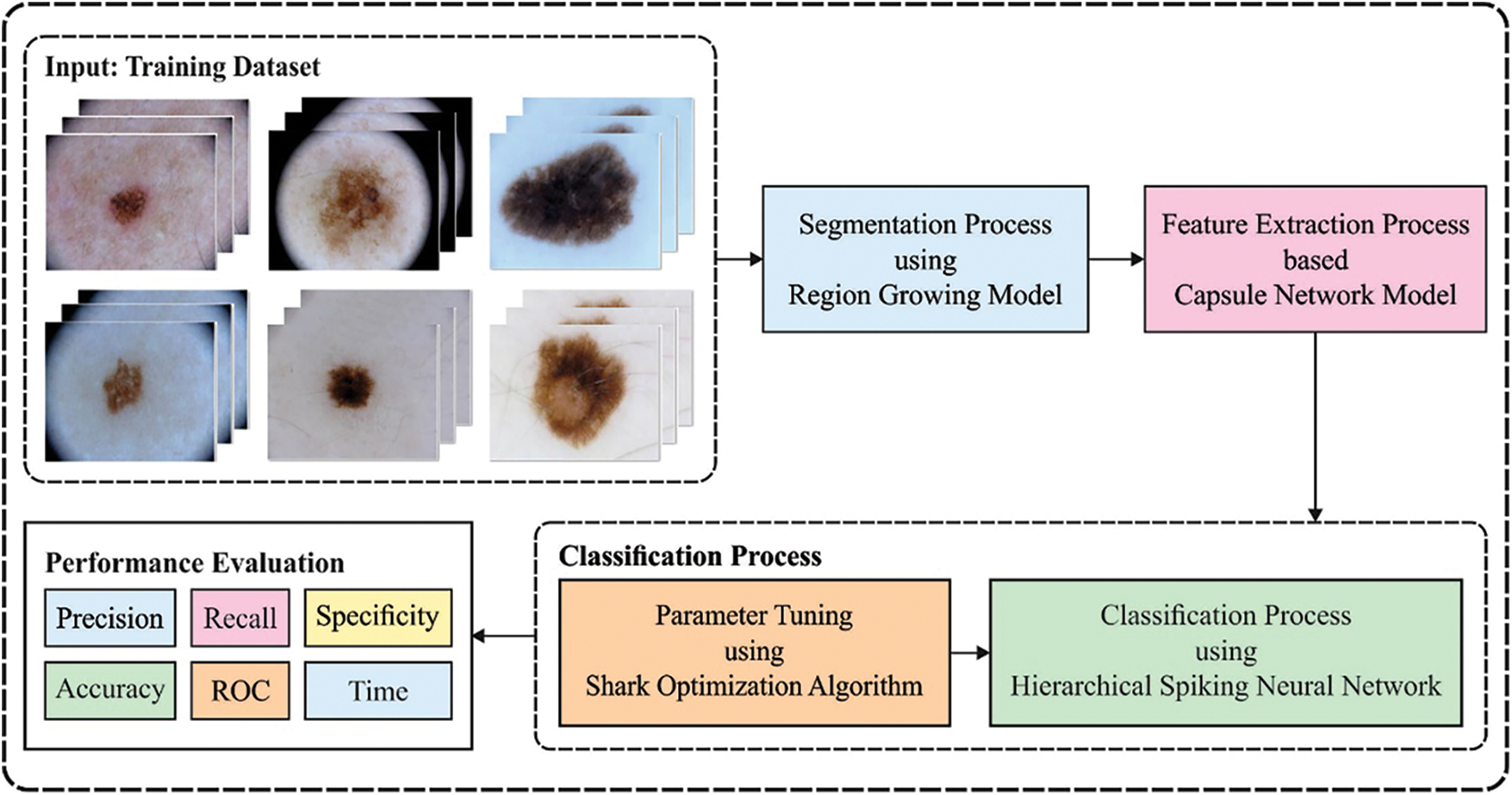
Figure 1: Overall block diagram of DCNN-HSNN model
3.1 Stage 1: Region based Segmentation Process
At the initial stage, the input medical images are segmented using region based segmentation technique. The steps involved in this process are listed as follows.
• Load the input images comprising infected and healthy portions.
• The coordinates of the initial point (pixel) of the growing need to be predefined by the users.
• The color intensities of the chosen point can be saved in the base value as seedval.
• Threshold values can be treated as threshval and it is set as 20% gray threshold of the whole image.
• The coordinate points of the initial pixel in the array named points are stored.
• The 8 pixels that exist in the initial pixel (neighboring pixels) are taken and the intensity of the color is checked whether it lies in the range of basic pixel color intensity in a particular accuracy, i.e., threshval. Every point is included in the point array offered by the subsequent criteria is satisfied [19]:
The above-mentioned criteria are tested for the newly present neighboring pixels which exist in the queue at the earlier step. These steps get iterated till the pixels are ineligible and reached the termination of the queue. At this point, the pixel in the point array can be considered as the infected region.
3.2 Stage 2: NADAM with CapsNet Based Feature Extraction Process
During feature extraction, the segmented image is fed into the CapsNet model, and features are extracted proficiently. The capsules have a group of neurons whose output is suggested as distinct features of the similar entity, and procedures the activation vectors. All the capsules contain pose matrix that demonstrates the occurrence of particular object place at a provided pixel and activation probabilities that demonstrate the length of vector. The activation vector way gathers the pose data of objects like place and orientation, but the activation vector length/magnitude measures the estimated possibility of an object of interest is developed. Upon rotating an image to instance, the activation vector is modified so but their length continues the similar. It might be several capsule layers. During the presented framework, it can beutilized an initial capsule layer. All the capsules forecast the parent capsule outcome and when this forecast has been consistent by parent capsule actual output, afterward the coupling coefficients amongst these 2 capsules improves. When ui implies the outcome capsule i, their forecast to parent capsules j has been defined in Eq. (3).
where
bij implies the log probability and fixed to zero, when the capsule i has been combined with capsule j primarily by agreement procedure at the beginning of routing. Therefore, the parent capsule input vector j has been calculated as Eq. (5).
Eventually, a non-linear squashing function has been utilized for normalizing the output vector of capsules to avoid them surpassing 1. Their length has been demonstrated as the probabilities by which a capsule is identify a provided feature. All the capsule’s last output has been defined as their primary vector value as demonstrated in Eq. (6).
where sj refers the entire input to capsule j and vj defines the output. According to the agreement amongst vj and
The routing co-efficient is improved with dynamic routing process to j-parent Capsule with influence of
where
3.3 Stage 3: SOA with HSNN Based Classification Process
At the final stage, the HSNN technique receives the derived feature vectors and performs classification process. The biological finding shows that the visual scheme might utilize feedback signals for highlighting the appropriate location. In this work, a SNN presented follows a hierarchical structure. Assume that an image is fed as input. The line detection layers include 2 pathways. The horizontal pathway has a Nh neuron array with a similar size as input neuron array. All the neurons have receptive fields equivalent to horizontal synapses strength matrix Wh. The vertical pathway has Nv neuron array with similar size as input neuron array. All the neurons have receptive field’s equivalent to vertical synapse strength matrix W. Thus, the spike rate map of neuron array
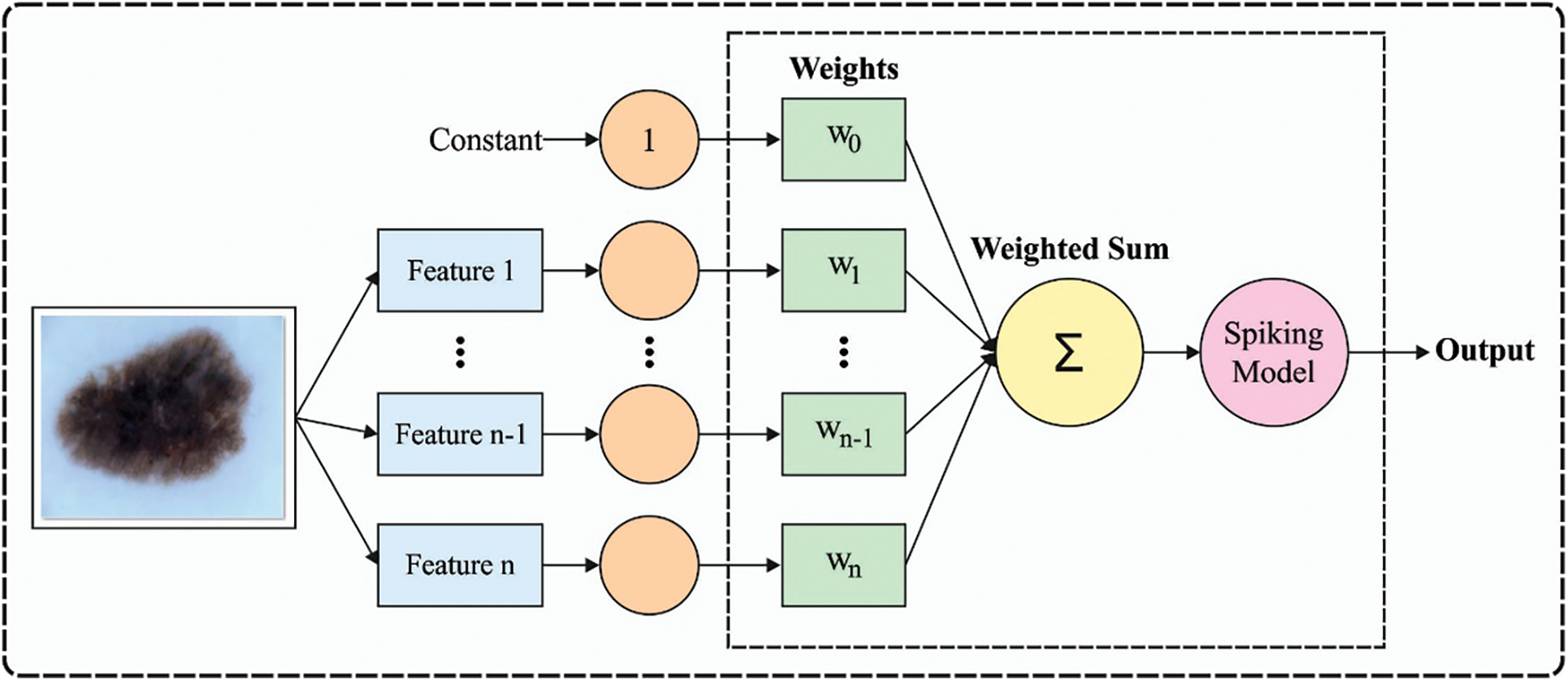
Figure 2: Framework of SNN model
The SNN employed in this study is made up of LIF neurons as follows:
However ai(tn) = ai(tn − 1) if f(ai(tn − 1) > 0
Let ai(tn) be the activation state of neurons i in time step n, j represent the index throughout neuron by outgoing synapsis leads to neurons i, wij indicates the weight of synapses from j to i neurons, as well, dij represent the delay time of synapses from j to i neurons. θ signifies the activation function for neurons i, that returns 1 when the variable is larger than/equivalent to neurons i activation threshold and 0 or else [23]. R indicates the refractory period as well tsi denotes the amount of time step as i neuron fired last. Instantly afterward firing, neuron enters a leakage state, where the neurons continue to output the similar output as earlier time step; f(x) specifies either the neurons are leaking or not. Each neuron in the networks is concurrently treated. For optimally tuning the parameters involved in the HSNN technique, the SOA is applied to it and consequently enhances the classification outcome. The shark follows a foraging performance that drives forward and rotates that is particularly effective in finding the prey. This optimized technique to inspired shark foraging is extremely effectual optimized technique. To some provided place, the sharks move at a speed to the particle which is further intense scent, therefore the primary velocity vectors were determined as:
The shark is inertia if it swims, therefore the velocity equation of all dimensions are determined as:
where j = (1, 2, …, ND), i = (1, 2, …, NP), and k = (1, 2, …, kmax); ND signifies the amount of dimensional; NP implies the amount of velocity vectors (size of shark populations); kmax demonstrates the amount of iteration [24]; OF stands for the objective function; ηk ∈ [0,1] refers the gradient coefficients; ak defines the weight coefficients, it can be also an arbitrary number amongst [0,1] and R1 and R2 denotes the 2 arbitrary numbers among 0 and 1.
The speed of sharks has been essential for avoiding the boundary and the particular speed restriction equation was explained as:
where βk implies the speed restrict factor of kth iteration.
A shark is a novel place
where Δtk denotes the time interval of kth iteration. Besides moving forward, the sharks generally rotate beside their path for looking to stronger odor particles and enhance their way of movement that is a real approach to moving. The rotating shark moves in a closed interval that is not essentially a circle. On the other hand, optimized sharks execute local search at all stages for finding optimum candidate solutions. The search equation to this place is as:
where m = (1, 2, …, M) defines the amount of points at all stages of place search; R3 refers the arbitrary number amongst −1 and 1. When the shark determines the stronger scent point under the rotation, it moves nearby the point as well as remains in the search direction. The place search equation has been explained as:
Since, it is obvious from the above equation,
The performance validation of the DCNN-HSNN technique is performed using HIS2828 [25] and ISIC2017 [26] datasets. The former dataset includes 2828 images with 1026 images under nervous tissue (NT) class, 484 images under connective tissue (CT) class, 804 images under epithelial tissue (ET) class, and 514 images into muscular tissue (MT) class. Besides, the later dataset has 2000 images with 374 images under Melanoma class and 1626 images under Nevus of Seborrheic (NS) Keratosis. Fig. 3 illustrates a few sample images.
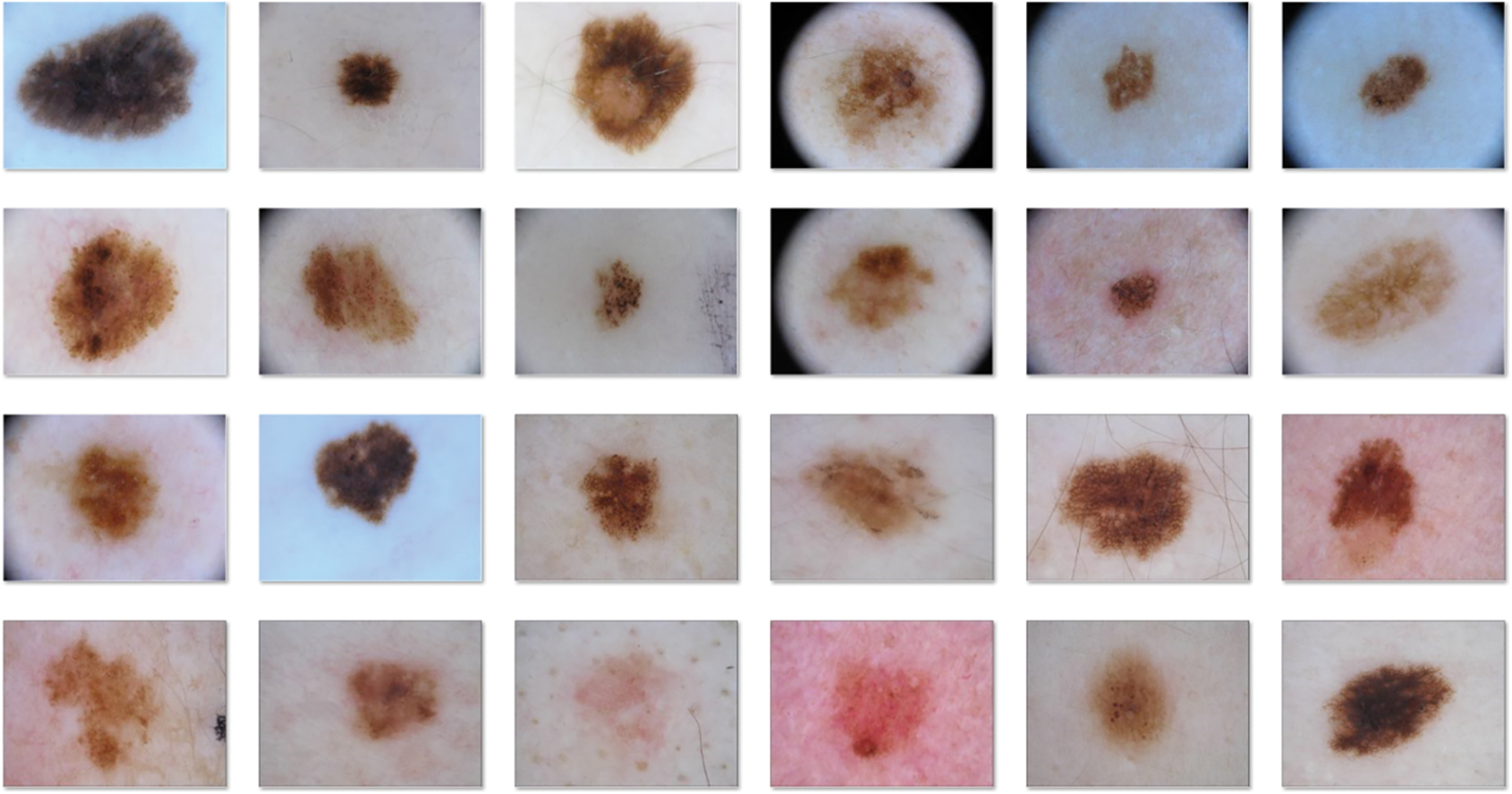
Figure 3: Sample images
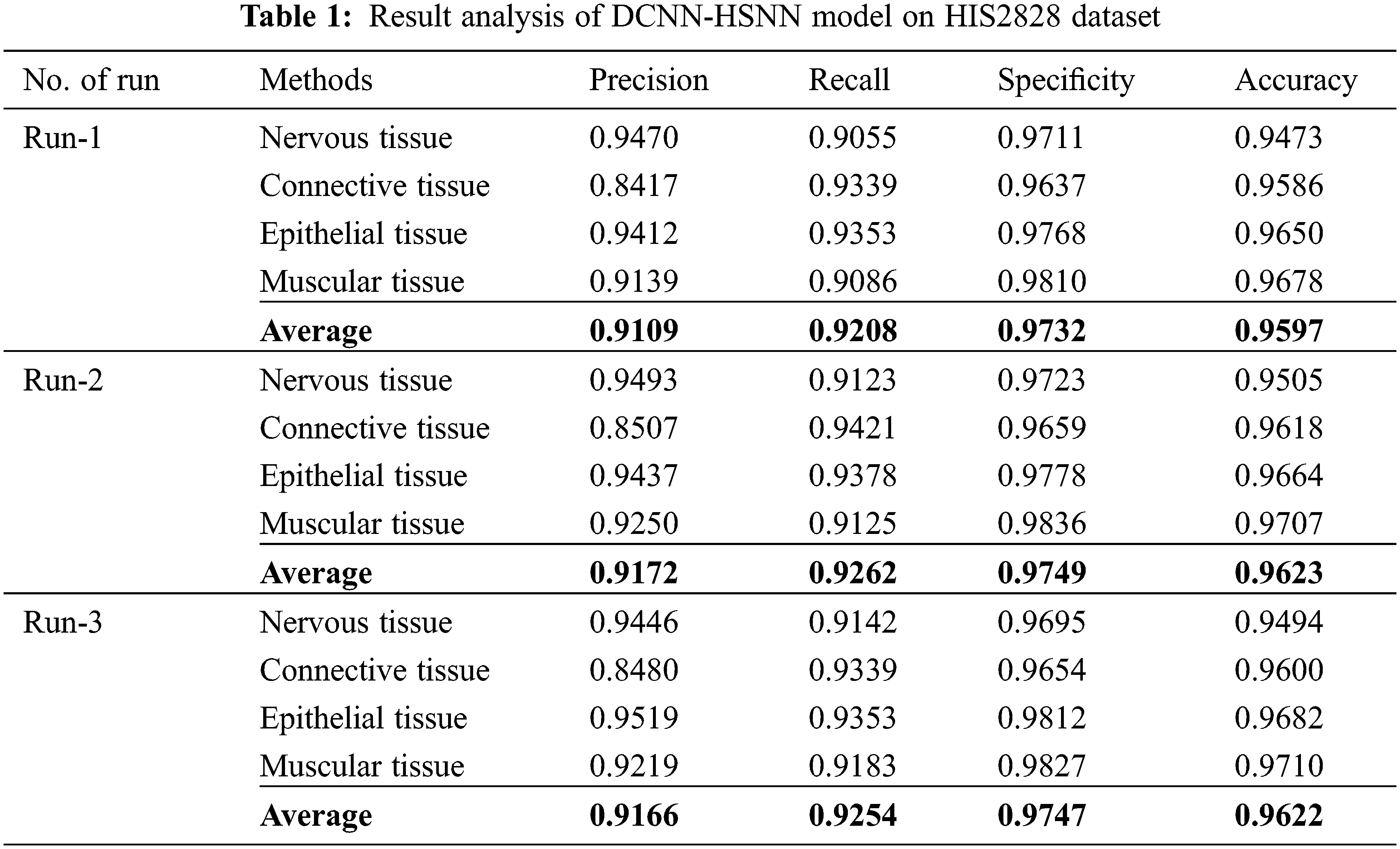
The confusion matrices produced by the DCNN-HSNN technique on the test HIS2828 dataset are given in Fig. 4 under three distinct runs. On the applied test run-1, the DCNN-HSNN technique has classified 929 images into NT, 452 images into CT, 752 images into ET, and 467 images into MT classes. At the same time, on the applied test run-2, the DCNN-HSNN approach has classified 936 images into NT, 456 images into CT, 754 images into ET, and 469 images into MT classes. Then, on the applied test run-3, the DCNN-HSNN manner has classified 938 images into NT, 452 images into CT, 752 images into ET, and 472 images into MT classes. The classification results analysis of the DCNN-HSNN technique on the applied HIS2828 dataset is given in Tab. 1. The results depicted that the DCNN-HSNN technique has accomplished proficient results on all the test runs. For instance, on run-1, the DCNN-HSNN technique has gained an average precision of 0.9109, recall of 0.9208, specificity of 0.9732, and accuracy of 0.9597. Moreover, on run-2, the DCNN-HSNN method has obtained an average precision of 0.9172, recall of 0.9262, specificity of 0.9749, and accuracy of 0.9623. Furthermore, on run-3, the DCNN-HSNN methodology has achieved an average precision of 0.9166, recall of 0.9254, specificity of 0.9747, and accuracy of 0.9622.
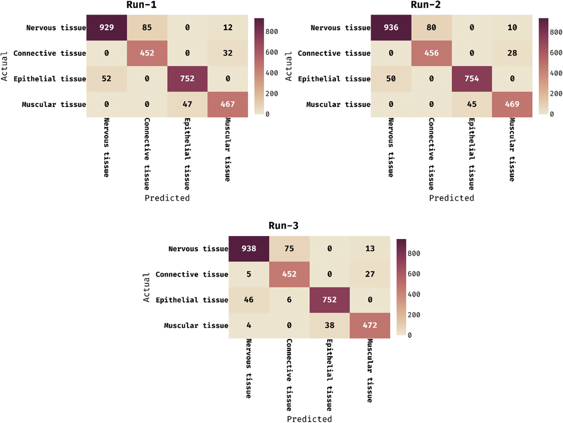
Figure 4: Confusion matrix of DCNN-HSNN technique on HIS2828 dataset
The accuracy graph of the DCNN-HSNN technique on the applied HIS2828 dataset is portrayed in Fig. 5. The obtained results demonstrated that the DCNN-HSNN technique has resulted in improved accuracy with an increase in epoch count. In addition, it is observed that the DCNN-HSNN technique has offered improved validation accuracy compared to training accuracy.
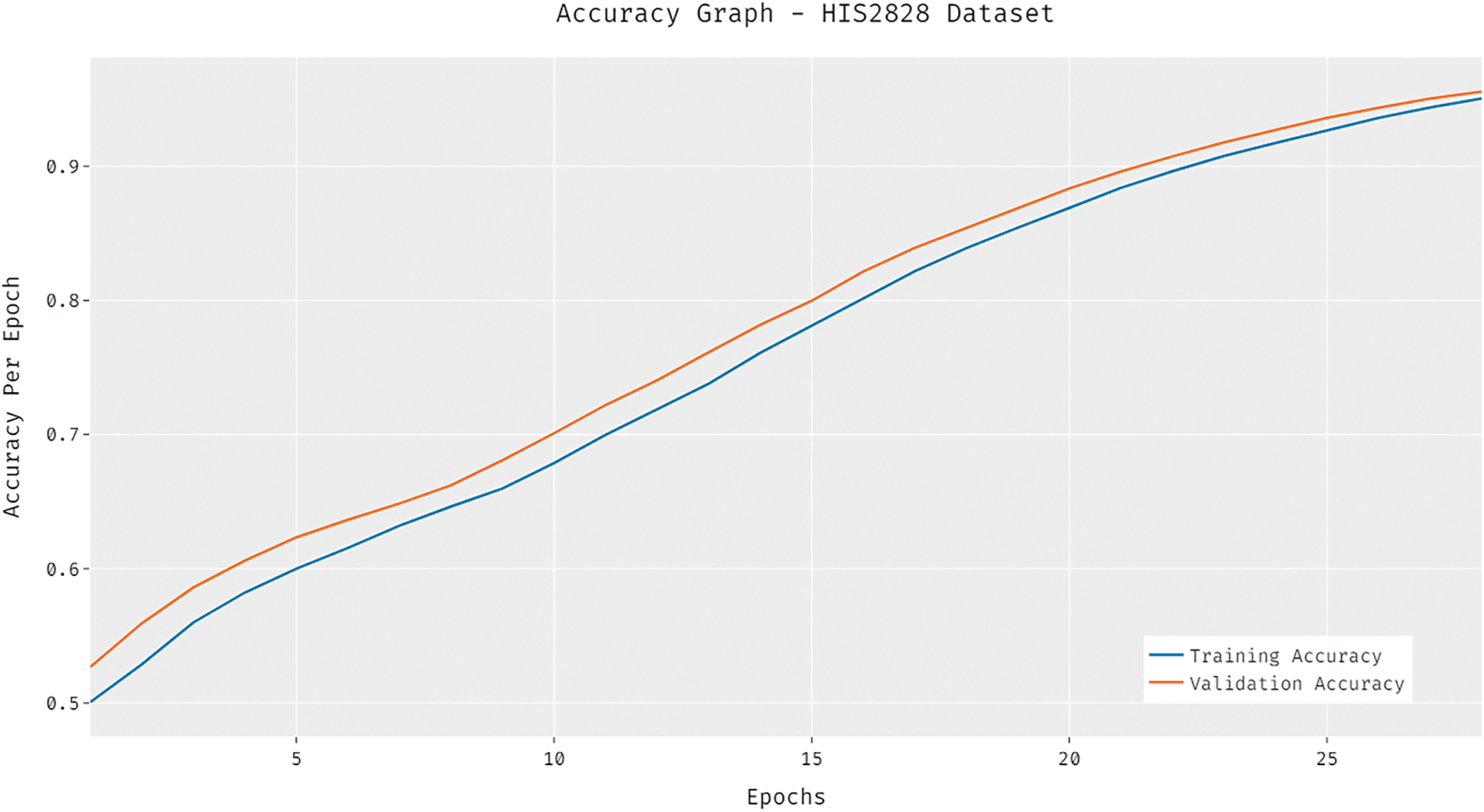
Figure 5: Accuracy analysis of DCNN-HSNN model on HIS2828 dataset
The loss graph of the DCNN-HSNN technique on the test HIS2828 dataset is depicted in Fig. 6. The attained results verified that the DCNN-HSNN technique has led to minimum loss with an increase in epoch count. Moreover, it is observed that the DCNN-HSNN technique has accomplished reduced validation loss over the training loss. The confusion matrices formed by the DCNN-HSNN algorithm on the test ISIC2017 dataset are provided in Fig. 7 under three different runs. On the applied test run-1, the DCNN-HSNN approach has classified 345 images into melanoma and 1528 images into NS keratosis classes. Followed by, on the applied test run-2, the DCNN-HSNN manner has classified 346 images into melanoma and 1529 images into NS keratosis classes. Eventually, on the applied test run-3, the DCNN-HSNN algorithm has classified 351 images into melanoma and 1541 images into NS keratosis classes.
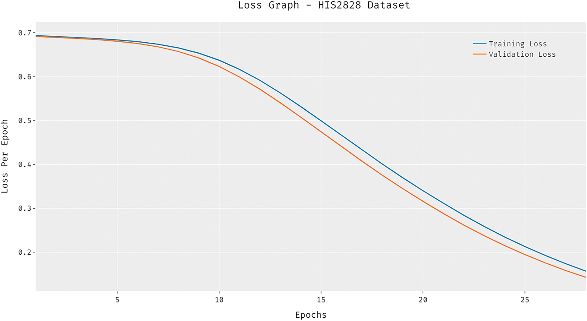
Figure 6: Loss analysis of DCNN-HSNN model on HIS2828 dataset
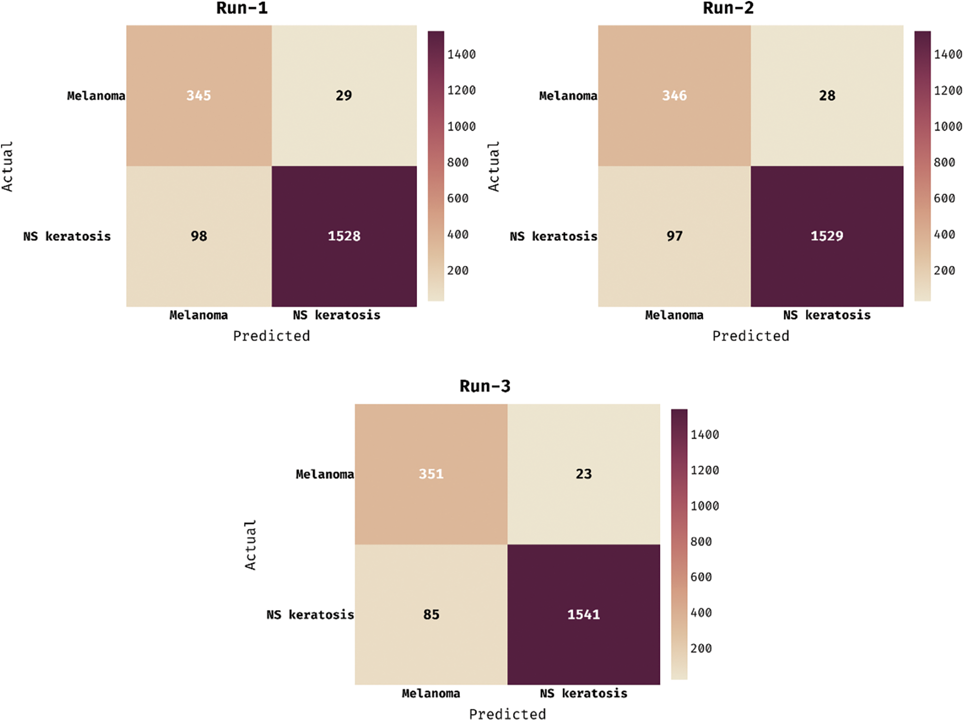
Figure 7: Confusion matrix of DCNN-HSNN technique on ISIC2017 dataset
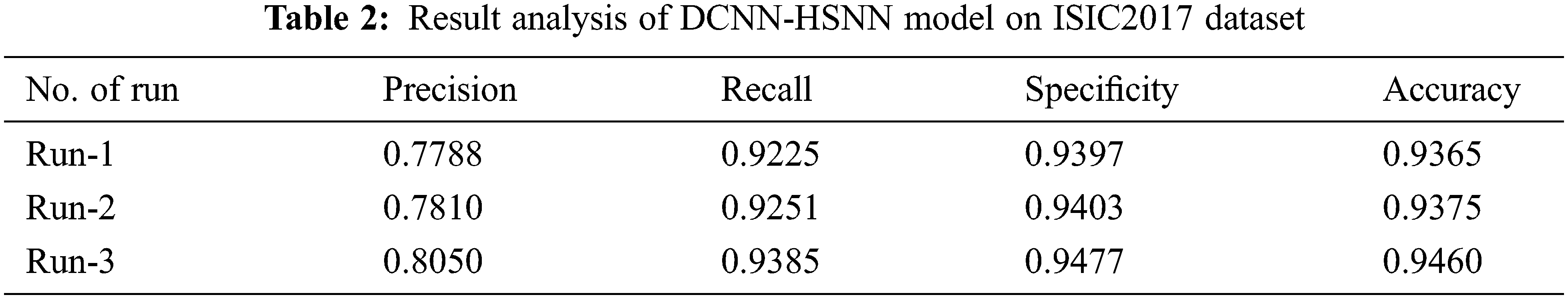
The classification outcome analysis of the DCNN-HSNN approach on the applied ISIC2017 dataset is offered in Tab. 2. The results outperformed that the DCNN-HSNN technique has accomplished proficient outcomes on all the test runs. For sample, on run-1, the DCNN-HSNN methodology has reached an average precision of 0.7788, recall of 0.9225, specificity of 0.9397, and accuracy of 0.9365. In addition, on run-2, the DCNN-HSNN technique has obtained an average precision of 0.7810, recall of 0.9251, specificity of 0.9403, and accuracy of 0.9375. Finally, on run-3, the DCNN-HSNN algorithm has attained an average precision of 0.8050, recall of 0.9385, specificity of 0.9477, and accuracy of 0.9460.
The accuracy graph of the DCNN-HSNN manner on the applied ISIC2017 dataset is depicted in Fig. 8. The achieved outcomes showcased that the DCNN-HSNN technique has resulted in enhanced accuracy with a maximum in epoch count. Besides, it can be clear that the DCNN-HSNN method has accessible increased validation accuracy related to training accuracy.
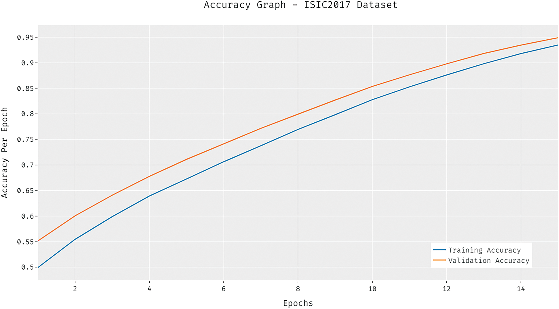
Figure 8: Accuracy analysis of DCNN-HSNN model on ISIC2017 dataset
The loss graph of the DCNN-HSNN algorithm on the test ISIC2017 dataset is demonstrated in Fig. 9. The gained outcomes stated that the DCNN-HSNN system has led to minimal loss with higher epoch count. Additionally, it can be obvious that the DCNN-HSNN approach has accomplished minimum validation loss over the training loss.
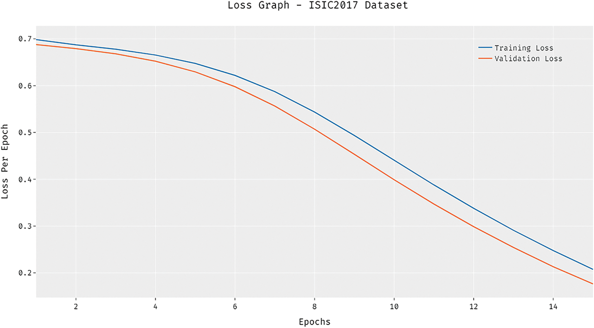
Figure 9: Loss analysis of DCNN-HSNN model on ISIC2017 dataset
A brief comparative results analysis of the DCNN-HSNN technique on the test HIS2828 dataset and ISIC dataset is reported in Tab. 3. The accuracy analysis of the DCNN-HSNN technique on the test HIS2828 dataset is shown in Fig. 10. The figure reported that the SVM-TF and Coding Network have offered minimal outcomes with the accuracy of 72.17% and 79.50% whereas the SVM-TDF and KPCA-FF techniques have obtained a slightly improved performance with the accuracy of 81.10% and 84.90% respectively. Followed by, the R-FF and CNMP techniques have accomplished reasonable accuracy of 90.20%. However, the presented DCNN-HSNN technique has resulted in a maximum accuracy of 96.22%.
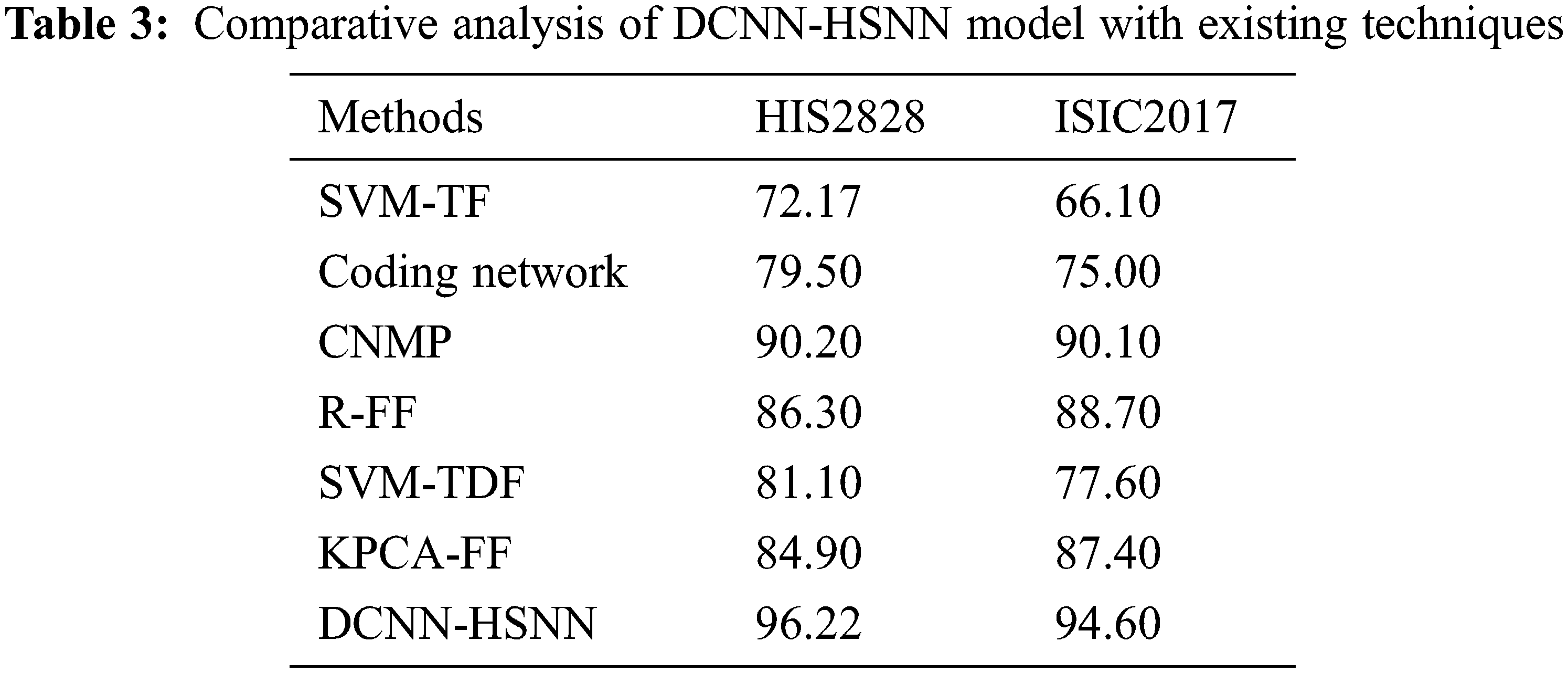
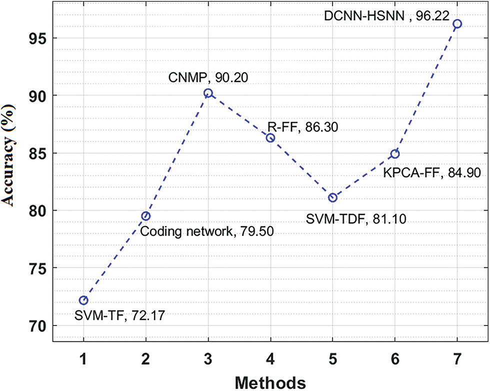
Figure 10: Accuracy analysis of DCNN-HSNN model on HIS2828 dataset
The accuracy analysis of the DCNN-HSNN method on the test ISIC2017 dataset is illustrated in Fig. 11. The figure described that the SVM-TF and Coding Network methods have obtainable least results with the accuracy of 66.10% and 75% whereas the SVM-TDF and KPCA-FF approaches have gained a somewhat superior efficiency with the accuracy of 77.60% and 87.40% correspondingly. Afterward, the R-FF and CNMP manners have accomplished reasonable accuracy of 88.70% and 90.10%. At last, the projected DCNN-HSNN algorithm has resulted in improved accuracy of 96.60%.
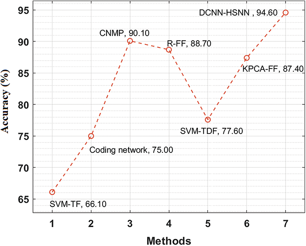
Figure 11: Accuracy analysis of DCNN-HSNN model on ISIC2017 dataset
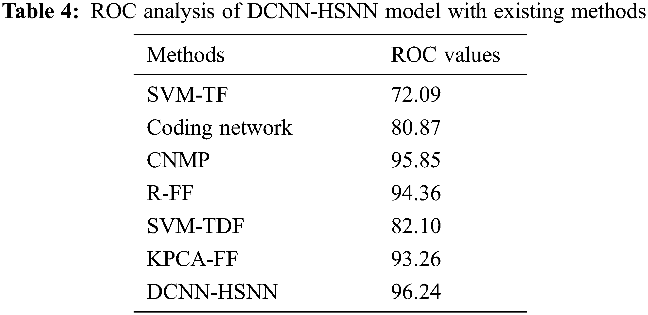
A detailed comparative outcomes analysis of the DCNN-HSNN approach with recent algorithms in terms of ROC is reported in Tab. 4. The result stated that the SVM-TF and Coding Network approaches have accessible worse outcomes with the ROC of 72.09 and 80.87 whereas the SVM-TDF and KPCA-FF manners have achieved a somewhat increased performance with the ROC of 82.10 and 93.26 correspondingly. At the same time, the R-FF and CNMP methods have accomplished reasonable ROC of 94.36 and 95.85. Finally, the proposed DCNN-HSNN methodologies have resulted in a superior ROC of 96.24.
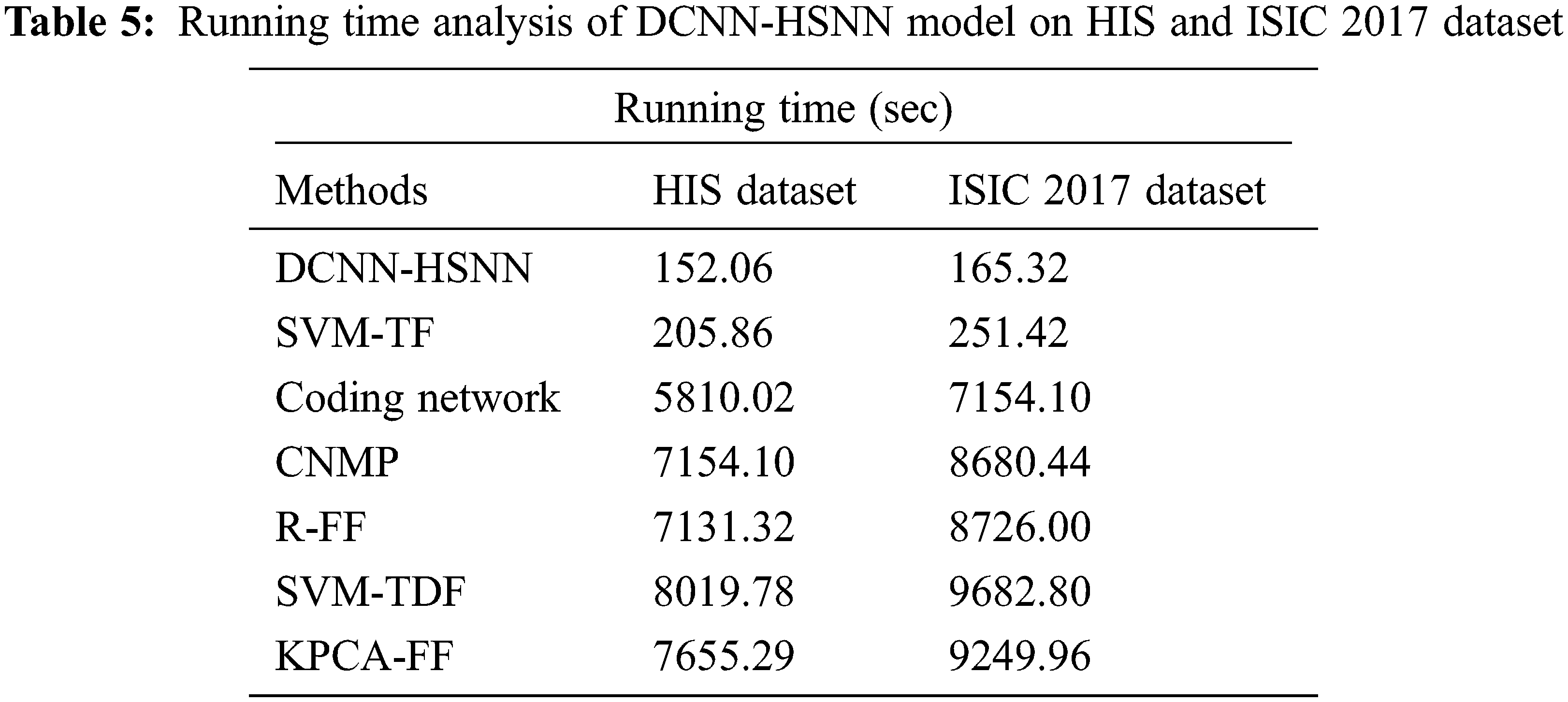
Finally, running time analysis of the DCNN-HSNN technique on the applied dataset is given in Tab. 5. The results demonstrated that the CNMP, R-FF, SVM-TDF, and KPCA-FF techniques have obtained ineffective outcomes with the maximum running time. In addition, the Coding Network has attained slightly reduced running time. Though the SVM-TF technique has resulted in a considerable running time of 205.86 and 251.42 s on the HIS2828 dataset and ISIC dataset, the DCNN-HSNN technique has required only a minimum of 152.06 and 165.32 s respectively.
From the detailed results analysis, it is evident that the DCNN-HSNN technique has resulted in an effective image classification outcome compared to other existing techniques.
In this study, a new DCNN-HSNN technique is derived for the medical image classification process. The DCNN-HSNN technique involves different stages of operations such as region growing based segmentation, CapsNet based feature extraction, NADAM based hyperparameter tuning, SNN based classification, and SSA based parameter optimization. The application of NADAM optimizer and SSA algorithm for parameter tuning process results in improved classification performance. The performance validation of the DCNN-HSSN technique is carried out on HIS2828 and ISIC2017 datasets. The experimental results highlighted the better performance of the DCNN-HSNN technique over the recent state of art techniques. Therefore, the DCNN-HSNN technique can be utilized as an effective tool for medical image classification and it can be deployed on Internet of Things enabled cloud environment in future.
Funding Statement: The authors received no specific funding for this study.
Conflicts of Interest: The authors declare that they have no conflicts of interest to report regarding the present study.
1. Q. Li, W. Cai, X. Wang, Y. Zhou, D. Feng et al., “Medical image classification with convolutional neural network,” in Proc. 13th Int. Conf. on Control Automation Robotics & Vision (ICARCV), IEEE, Singapore, pp. 844–848, 2014. [Google Scholar]
2. M. L. Antonie, O. R. Zaiane and A. Coman, “Application of data mining techniques for medical image classification,” in Proc. Second Int. Conf. on Multimedia Data Mining, San Jose, CA, pp. 94–101, 2001. [Google Scholar]
3. S. N. Deepa and B. A. Devi, “A survey on artificial intelligence approaches for medical image classification,” Indian Journal of Science and Technology, vol. 4, no. 11, pp. 1583–1595, 2011. [Google Scholar]
4. S. C. Hoi, R. Jin, J. Zhu and M. R. Lyu, “Batch mode active learning and its application to medical image classification,” in Proc. of the 23rd Int. Conf. on Machine Learning, Pennsylvania, USA, pp. 417–424, 2006. [Google Scholar]
5. A. Kumar, J. Kim, D. Lyndon, M. Fulham and D. Feng, “An ensemble of fine-tuned convolutional neural networks for medical image classification,” IEEE Journal of Biomedical and Health Informatics, vol. 21, no. 1, pp. 31–40, 2016. [Google Scholar]
6. R. J. Ramteke and K. Y. Monali, “Automatic medical image classification and abnormality detection using k-nearest neighbor,” International Journal of Advanced Computer Research, vol. 2, no. 4, pp. 190, 2012. [Google Scholar]
7. E. Miranda, M. Aryuni and E. Irwansyah, “A survey of medical image classification techniques,” in Proc. Int. Conf. on Information Management and Technology (ICIMTech), IEEE, Bandung, Indonesia, pp. 56–61, 2016. [Google Scholar]
8. P. Rajendran and M. Madheswaran, “Hybrid medical image classification using association rule mining with decision tree algorithm,” Journal of Computing, vol. 2, no. 1, pp. 127–136, 2010. [Google Scholar]
9. C. M. Dourado, S. P. P. da Silva, R. V. M. da Nobrega, P. P. Rebouças Filho, K. Muhammad et al., “An open IoHT-based deep learning framework for online medical image recognition,” IEEE Journal on Selected Areas in Communications, vol. 39, no. 2, pp. 541–548, 2020. [Google Scholar]
10. Z. Lai and H. Deng, “Medical image classification based on deep features extracted by deep model and statistic feature fusion with multilayer perceptron,” Computational Intelligence and Neuroscience, vol. 1, no. 2018, pp. 1–24, 2018. [Google Scholar]
11. S. S. Yadav and S. M. Jadhav, “Deep convolutional neural network based medical image classification for disease diagnosis,” Journal of Big Data, vol. 6, no. 1, pp. 1–18, 2019. [Google Scholar]
12. E. Korot, Z. Guan, D. Ferraz, S. K. Wagner, G. Zhang et al., “Code-free deep learning for multi-modality medical image classification,” Nature Machine Intelligence, vol. 3, no. 4, pp. 288–298, 2021. [Google Scholar]
13. J. Zhang, Y. Xie, Q. Wu and Y. Xia, “Medical image classification using synergic deep learning,” Medical Image Analysis, vol. 54, pp. 10–19, 2019. [Google Scholar]
14. R. J. S. Raj, S. J. Shobana, I. V. Pustokhina, D. A. Pustokhin, D. Gupta et al., “Optimal feature selection-based medical image classification using deep learning model in internet of medical things,” IEEE Access, vol. 8, pp. 58006–58017, 2020. [Google Scholar]
15. X. Ma, Y. Niu, L. Gu, Y. Wang, Y. Zhao et al., “Understanding adversarial attacks on deep learning based medical image analysis systems,” Pattern Recognition, vol. 110, pp. 107332, 2021. [Google Scholar]
16. A. Smailagic, P. Costa, A. Gaudio, K. Khandelwal, M. Mirshekari et al., “O-MedAL: Online active deep learning for medical image analysis,” Wiley Interdisciplinary Reviews: Data Mining and Knowledge Discovery, vol. 10, no. 4, pp. e1353, 2020. [Google Scholar]
17. R. Ashraf, M. A. Habib, M. Akram, M. A. Latif, M. S. A. Malik et al., “Deep convolution neural network for big data medical image classification,” IEEE Access, vol. 8, pp. 105659–105670, 2020. [Google Scholar]
18. S. Hicks, M. Riegler, K. Pogorelov, K. V. Anonsen, T. de Lange et al., “Dissecting deep neural networks for better medical image classification and classification understanding,” in Proc. IEEE 31st Int. Symposium on Computer-Based Medical Systems (CBMS), Karlstad, Sweden, pp. 363–368, 2018. [Google Scholar]
19. J. S. Nabipour, A. Khorshidi and B. Noorian, “Lung tumor segmentation using improved region growing algorithm,” Nuclear Engineering and Technology, vol. 21, no. 2020, pp. 1–21, 2020. [Google Scholar]
20. S. Panigrahi, J. Das and T. Swarnkar, “Capsule network based analysis of histopathological images of oral squamous cell carcinoma,” Journal of King Saud University-Computer and Information Sciences, vol. 12, no. 2020, pp. 1–24, 2020. [Google Scholar]
21. T. Dozat, “Incorporating nesterov momentum into adam,” ICLR Workshop, vol. 1, pp. 1–18, 2016. [Google Scholar]
22. Q. Wu, T. M. McGinnity, L. Maguire, R. Cai and M. Chen, “Simulation of visual attention using hierarchical spiking neural networks,” in Proc. Int. Conf. on Intelligent Computing, Springer, Berlin, Heidelberg, pp. 26–31, 2011. [Google Scholar]
23. A. Bennett and A. White, “Dynamical properties of spiking neural networks with small world topologies,” Procedia Computer Science, vol. 190, pp. 71–81, 2021. [Google Scholar]
24. L. Wang, X. Wang, Z. Sheng and S. Lu, “Multi-objective shark smell optimization algorithm using incorporated composite angle cosine for automatic train operation,” Energies, vol. 13, no. 3, pp. 714, 2020. [Google Scholar]
25. Z. Lai and H. Deng, “Medical image classification based on deep features extracted by deep model and statistic feature fusion with multilayer perceptron,” Computational Intelligence and Neuro Science, vol. 2018, no. 2061516, pp. 1–18, 2018. [Google Scholar]
26. N. Codella, D. Gutman, M. E. Celebi, B. Helba, M. A. Marchetti et al., “Skin lesion analysis toward melanoma detection,” in International Symposium on Biomedical Imaging (ISBI), Melbourne, Australia, pp. 1–32, 2017. [Google Scholar]
 | This work is licensed under a Creative Commons Attribution 4.0 International License, which permits unrestricted use, distribution, and reproduction in any medium, provided the original work is properly cited. |