Computer Systems Science & Engineering DOI:10.32604/csse.2023.026467
Article

Intelligent Smart Grid Stability Predictive Model for Cyber-Physical Energy Systems

Ashit Kumar Dutta1,*, Manal Al Faraj1, Yasser Albagory2, Mohammad zeid M Alzamil1 and Abdul Rahaman Wahab Sait3

1Department of Computer Science and Information Systems, College of Applied Sciences, AlMaarefa University, Ad Diriyah, Riyadh, 13713, Kingdom of Saudi Arabia
2Department of Computer Engineering, College of Computers and Information Technology, Taif University, Taif, 21944, Kingdom of Saudi Arabia
3Department of Archives and Communication, King Faisal University, Al Ahsa, Hofuf, 31982, Kingdom of Saudi Arabia
*Corresponding Author: Ashit Kumar Dutta. Email: adotta@mcst.edu.sa
Received: 27 December 2021; Accepted: 15 February 2022

Abstract: A cyber physical energy system (CPES) involves a combination of processing, network, and physical processes. The smart grid plays a vital role in the CPES model where information technology (IT) can be related to the physical system. At the same time, the machine learning (ML) models find useful for the smart grids integrated into the CPES for effective decision making. Also, the smart grids using ML and deep learning (DL) models are anticipated to lessen the requirement of placing many power plants for electricity utilization. In this aspect, this study designs optimal multi-head attention based bidirectional long short term memory (OMHA-MBLSTM) technique for smart grid stability prediction in CPES. The proposed OMHA-MBLSTM technique involves three subprocesses such as pre-processing, prediction, and hyperparameter optimization. The OMHA-MBLSTM technique employs min-max normalization as a pre-processing step. Besides, the MBLSTM model is applied for the prediction of stability level of the smart grids in CPES. At the same time, the moth swarm algorithm (MHA) is utilized for optimally modifying the hyperparameters involved in the MBLSTM model. To ensure the enhanced outcomes of the OMHA-MBLSTM technique, a series of simulations were carried out and the results are inspected under several aspects. The experimental results pointed out the better outcomes of the OMHA-MBLSTM technique over the recent models.

Keywords: Stability prediction; smart grid; cyber physical energy systems; deep learning; data analytics; moth swarm algorithm

1  Introduction

In recent years, Digitalization and Automation have become significant topics in the energy sector, as modern energy system increasingly relies on information and communication technologies (ICT) to integrate smart controls with hardware framework [1]. In this regard, applications such as smart buildings and smart grids have pioneered the interweaving of software and hardware mechanisms, working on distinct spatial and temporal scales and frequently across the boundary of conventional engineering domain. With the development of cyber–physical systems (CPS) as a transdisciplinary field, this modern energy system could be categorized as cyber–physical energy systems (CPES), incorporating the development and related research within a larger context. A significant factor of the development and research associated with CPS is to connect the gap between the computer science and traditional engineering domains [2]. Especially, it applies CPES, where the interrelated engineering domain has reliable methods to design complex and large models. But, with the emergence of renewable and distributed resources and the incorporation of energy systems across the conventional boundaries of engineering domain, these proven methodologies are required extension and are being challenged. The integration of ubiquitous amounts of data and the inclusion of intelligent control strategies that are facilitated by the concept of CPES is predicted to be a significant facilitator for the predicted transformation of the energy systems [3–5]. Fig. 1 shows the structure of CPS system [6].

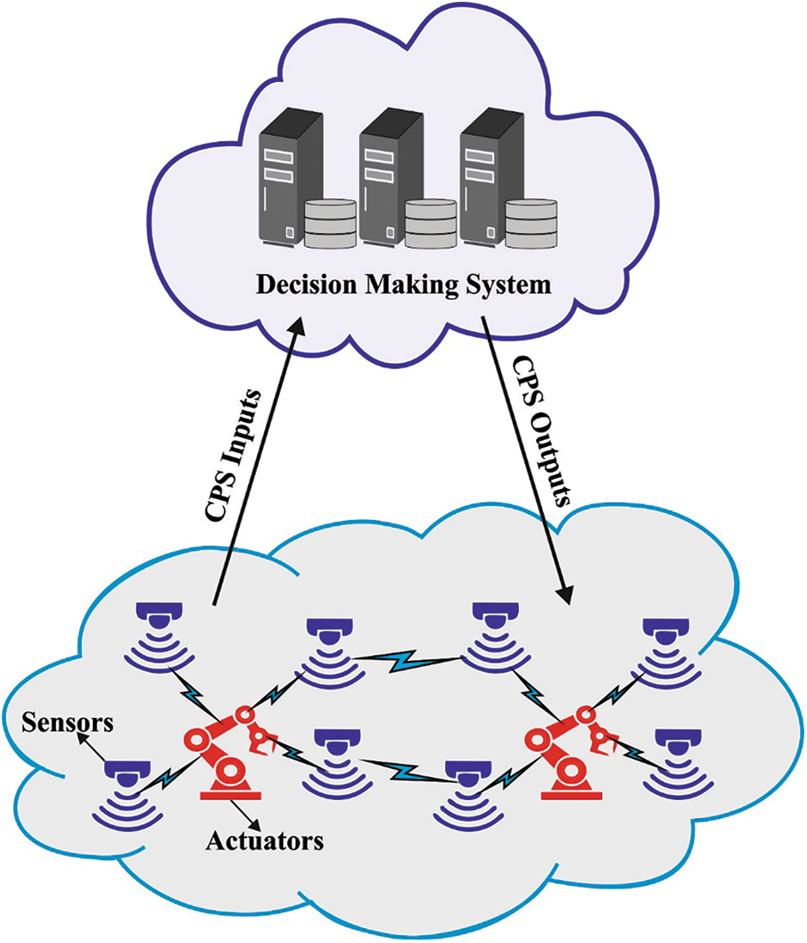
Figure 1: Overview of CPS systems

There has been comprehensive study on the grid network for the distribution of power over different locations efficiently. One of these methods is the smart grid that employs ICT for aggregating data concerning the behavior of consumers to generate a context-aware scheme that could allocate the energy efficiently. Smart grids utilizing Artificial Intelligence (AI) technique are predicted for reducing the requirement to deploy additional power stations for electrical energy consumption. Also, the Smart grid uses renewable resources to be plugged securely into the grid system to appendage the source of electricity. The cyber-physical smart grids have experienced substantial damage on transformers, power lines, amongst others; also, cyber-attack and cyberespionage have been reported in real-life incidents. Such difficulties have driven the researches in defense and cyber-physical attack of the smart grids from control, information, power, and several more security-related researches, which leads to unified cyber-physical security perspectives. Smart grids, that could forecast energy consumption is essential need. This could be achieved with the applications of Machine Learning (ML) algorithm [7–9] on the generated data from the grid system. Smart grids could assist in making the electricity price much cheaper and reducing pollution [10].

Wei et al. [11] presented a DL-based cyber-physical scheme to mitigate and identify the data corruption in the problem of preserving the transient stability of Wide Area Monitoring Systems (WAMS). The presented method executes the DL method for analyzing the real-world data measurement from the geographically distributed Phasor Measurement Unit (PMU) and leverages the physical coherence in the electrical energy system to detect and probe the corruption of information. In [12], a NN system-based fault detection method is employed to track and detect fault data injection attacks on the cooperative adaptive cruise control system of a platoon of interconnected vehicles in real time. A DSS method has been proposed for reducing the severity and probability of subsequent accidents.

In [13], many advanced ML methods like, SVM, KNN, LR, NB, NN, and DT classifiers, were installed to predict the SG stability. The SG data set utilized in this work is open-source data gathered from UC Irvine (UCI) ML source. Jafari et al. [14] proposed a new stability state forecaster based cascaded FFNN method. The presented strategy focuses on identifying anomalies as a result of physical or cyber disruptions as an earlier indication of instability. The presented method uses cascaded connection for increasing the predictive accuracy. The Polak-Ribiére formula and conjugate gradient backpropagation are exploited for training procedures. In [15], ML based edge computation could identify the seriousness of the warning, detect the network region of interest and ignite the performance of the transient condition perdition. The transient state prediction forecasts the incoming failure in real time when the timing window permits potential protective actuation.

Haija et al. [16] proposed a novel wide-ranging detection method that applies ML framework to classify stability records in smart grid systems. Especially, seven ML frameworks are examined, involving DT, optimized SVM, NB, LR, KNN, LDC, and ensemble boosted classifiers (EBC). Singh et al. [17] introduced a methodology and architecture to develop a cyber-physical anomaly detection system (CPADS) that employs synchrophasor properties and measurements of networking packets for detecting communication failure attacks and data integrity on control signals and measurement in CRAS. The presented model employs a rules-based model for selecting appropriate input feature, employs decision tree (DT) algorithms and variational mode decomposition (VMD) for developing various classification system, and perform event detection with rules-based decision logic.

This study designs optimal multi-head attention based bidirectional long short term memory (OMHA-MBLSTM) technique for smart grid stability prediction in CPES. The proposed OMHA-MBLSTM technique involves three subprocesses such as min-max normalization based pre-processing, prediction, and hyperparameter optimization. Moreover, the MBLSTM model is applied for the prediction of stability level of the smart grids in CPES. Furthermore, moth swarm algorithm (MHA) is utilized for optimally modifying the hyperparameters involved in the MBLSTM model. For ensuring the improved performance of the OMHA-MBLSTM technique, a series of simulations were carried out and the results are inspected under several aspects.

2  The Proposed Model

In this study, an effective OMHA-MBLSTM technique has been developed to predict the stability level of the smart grids in the CPES environment. The proposed OMHA-MBLSTM technique involves three subprocesses (as shown in Fig. 2) as min-max normalization based pre-processing, MBLSTM based prediction, and MHA based hyperparameter optimization. The design of MHA helps to appropriately elect the hyperparameters and it leads to enhanced predictive outcomes.

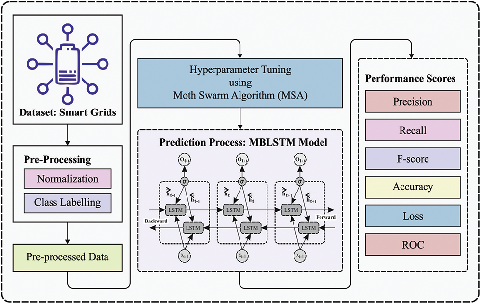
Figure 2: Working process of OMHA-MBLSTM technique

2.1 Pre-processing

First, the electricity grid dataset from different power generating units is aggregated. The dataset is then normalized using min-max normalization. During this process, the minimum and maximum values of the data are obtained and replaced by using Eq. (1).

L¯=l−min(X)max(X)−min(X)(newmin(X)−newmax(X))+newmin(X) (1)

where X denotes the parameter that exists in the data, min(X) and max(X) represents the lower and upper levels of the attribute values, L¯ represents the upgraded values of entries, l implies the earlier value in the data and newmin(X)andnewmax(X) indicates the value of minimum and maximum limits correspondingly.

2.2 Prediction Using MBLSTM Model

Next to the pre-processing stage, the MBLSTM model is utilized to perform the stability prediction process [18]. The RNN is a distinct structure of NN in MLP. In RNN splits weight and is particularly appropriate to domain of order analysis like language translation as well as semantic understanding. The hidden layer Ht at time step t is not only based on the existing input as in preceding hidden layer that is estimated as:

Ht=f(XtW+Ht−1U+α) (2)

where f refers to the activation function and α signifies the bias. The output Ot at the time step t has calculated as:

Ot=g(HtS+β) (3)

where g stands for the activation function and β is a bias. To lengthy series, it is a vital issue with RNN, for instance, vanishing gradients. Amongst every solution to vanishing gradients, the LSTM is most optimum. The LSTM has candidate memory cell and 3 gates: output, forget, and input gates. The forget gate Ft, input gate It, and output gate Pt at time step t are calculated correspondingly as:

Ft=σ(XtWx,f+Ht−1Wh,f+bf) (4)

It=σ(XtWx,i+Ht−1Wh,i+bi) (5)

Pt=σ(XtWx,0+Ht−1Wh,0+bo) (6)

where Wχ,f and Wh,f denotes the weights of LSTM in input-forget gate and in hidden layer to forget gate correspondingly. Wx,i and Wh,i refers to the association weights under the input-input gate and the hidden layer to the input gate correspondingly. Wx,0 and Wh,0 signifies the connect weights under the input-output gates and the hidden layer to the output gate correspondingly. bf, bi, and bo signifies the bias of forgetting, input, as well as output gates correspondingly. σ represents the activation function. The candidate memory cell has estimated as:

C¯= tanh (XtWx,c+Ht−1Wh,c+bc) (7)

where Wx,c and Wh,c defines the weight of LSTM under input to candidate memory and the hidden layer to candidate memory correspondingly, and bc refers to the bias. The memory cell at time step t has measured as:

Ct=Ft⊗Ct−1+It⊗C¯ (8)

where ⊗ determined as element-wise multiplication. The hidden layer is upgraded as:

Ht=It⊗ tanh (Ct) (9)

The preceding RNN has forwarded. The output at time step t is only based on prior input and hidden layer. Moreover, the output can be useful to last input as well as hidden layer. The forward hidden layer at time step t has evaluated as:

Htf=σ(XtWx,hf+Ht−1fWh,hf+bhf) (10)

but the backward hidden layer gas measured as:

Htb=σ(XtWx,hb+Ht+1bWh,hb+bhb) (11)

The output at time step t is calculated as:

Ot=[Htf, Htb]Wh,0+bo (12)

Attention is process to enhance the outcome of RNN based techniques, and the computation of attention has mostly separated into 3 stages. A 1st stage is for utilizing the attention function F for scoring query as well as key to obtaining si. The 2 most common attention functions were additive attention as well as dot-product attention [19]; during this case, it can utilize the former. The 2nd stage is to utilize softmax function for normalizing the score outcome si, for obtaining the weight ai. The 3rd stage is for calculating attention that is weighted average of every value as well as weight ai. The Multi-head attention is enhanced by the standard attention process, thus all heads are removed the feature of query and key from various subspaces. Specifically, these features derive in Q and K that are projections of query as well as key from the subspaces. The operation was implemented when all heads and entire of h times required that carried out. It can be stated that under the multi-head attention method, the attention function is scaled dot-product function that is similar to the classical attention process, apart from regulating scaling factor. During the experiment, h requires that always debugged for determining the most useful value to tasks. Eventually, the outcomes that were returned from all heads were concatenated and linearly changed to attain multi-head attention. At last, it can be sent the vector in the preceding layer to densely connected layer. It can be utilized ReLu function as activation function for completing the non-linear conversion. Finally the densely connected layer, it is execute softmax operation on the output of preceding layer, and lastly attains classification outcomes.

2.3 Hyperparameter Tuning Using MHA

To enhance the predictive outcomes of the MBLSTM model, the MHA is employed. The nighttime performance of moths is simulated to MHA has established in [20]. During this technique, the exploration and exploitation balance examine a separation of candidate solutions developing the populations. As if other meta-heuristics, it can be initialized a population:

xij=rand⋅(uj−lj)+lj,∀i∈{,2,n},j∈{,2,d} (13)

where u and l refers the upper as well as lower limits of search space, xi indicates the candidate solution, n denotes the population size, d stands for the problem dimensional, and rand implies the arbitrary value taken in uniform distribution. For generating the pathfinders crossover it can be essential for calculating the dispersal degree and variation coefficient at iteration t:

σjt=1np∑i=1np⁡(xijt−Pjt)2Pjt  (14)

μt=1d∑j=1d⁡σjt (15)

where np represents the amount of pathfinders, and

Pjt=1np∑i=1np⁡xiij (16)

During the MHA crossover points were individuals with minimal dispersal values dependent upon:

j∈cp if σjt≤μt (17)

After that only nc ∈ cp crossover point was employed for generating novel sub-trial pathfinder vectors vp→=[vp1,vp2, …,vpnc] under the novel pathfinder χp→=[χp1,χp2, …,χpnc] as follows:

vpt→=→xr1t+Lp1t⋅(xr2t→−xr3t→)+Lp2t⋅(xr4t→−xr5t→)

∀r1≠r2≠r3≠r4≠r5≠p∈{1,2, …, np} (18)

where Lpl and Lp2 implies the independent variable calculated in the Lévy α-stable distribution. The group of indexes r suppose that only chosen in the pathfinder solution, and individuals places were upgraded utilizing the mutated variable removed in the sub-trail vector based on subsequent formula:

Vpjt={vpjrif j∈cpxpjtif j∉cp (19)

Lastly, the MHA executes a chosen approach among the trial as well as original pathfinders determined as:

xpt+1→={xpt→i if f(Vpt→)≥f(xpt→)vpt→ otherwise (20)

The probability of choosing the following pathfinder was determined as:

pp=fitp∑p=1np⁡fitp (21)

That utilizes the luminescence intensity computed as subsequent formula:

fitp={11+fp if fp≥01+|fp| otherwise  (22)

In the pathfinder, nf those were chosen as prospectors; this number is dynamically changed as under the subsequent formula:

nf=round((n−np)×(1−tT)) (23)

With T being the maximal iteration number. For simulating prospector moth moving from spiral manner nearby pathfinder (their natural counterpart), the MHA utilizes the subsequent determined:

xit+1=|xit−xpt|⋅eθ⋅cos2πθ+xpt∀p∈{1,2, …, np};i∈{np+1, np+2, …, nf} (24)

where θ∈[r, 1] signifies the arbitrary number employed for giving the spiral procedure to prospector path, but r = −1 − t/T⋅

The onlooker is a moth with minimum luminescent intensity moving near the shiniest source of light; during the MHA, the onlooker's stage was employed for intensifying the exploitation of promissory spots of search spaces. The onlooker group is more separated based on 2 movement rules: Gaussian walks, and associative learning process with immediate memory. At the beginning, the onlooker in the actual iteration was attained as:

xit+1=xit+ϵ1+[ϵ2⋅bestgt−ϵ3⋅xit],∀i∈{,2,⋯,no} (25)

where ɛ2 and ɛ3 defines the uniformly distributed arbitrary numbers, bestg refers the global optimum candidate solutions, no = round(nu/2) represents the amount of onlookers which executes a Gaussian movement, nu stands for the amount of onlookers, and ɛ1 signifies the normal arbitrary number computed as:

ϵ1∼random(size(d))⊕N(bestt)(xit−bestgt)) (26)

The performance of moths regarding associative learning as well as short-term memory is upgraded based on:

xit+1=xit+0.001⋅G+(1−gG)⋅ϵ2⋅(besdp−xit)+

(2gG)⋅ϵ3⋅(bestpt−xit),∀i∈{1,2,…,nm} (27)

with nm = nu − no being the amount of onlookers which executes associative learning and short-term memory, 1 − g/G refers to the cognitive factor, 2g/G signifies the social issue, bestp signifies the optimum light source under the pathfinder group and G∼N(xit−ximin,ximax−xit) .

3  Performance Validation

This section examines the predictive outcome of the OMHA-MBLSTM technique over the other techniques. Tab. 1 provides a brief results analysis of the OMHA-MBLSTM technique with recent methods under training and testing processes. Fig. 3 investigates the comparative training accuracy and testing accuracy of the OMHA-MBLSTM technique. The results show that the RNN model has showcased poor outcomes with lower training accuracy and testing accuracy. Followed by, the GRU and LSTM models have obtained slightly improved training accuracy and testing accuracy. In line with, the MLSTM and MHA-BLSTM models have accomplished near optimal training accuracy and testing accuracy. However, the OMHA-MBLSTM technique has outperformed the other DL models with the increased training accuracy and testing accuracy of 0.9967 and 0.9971 respectively.

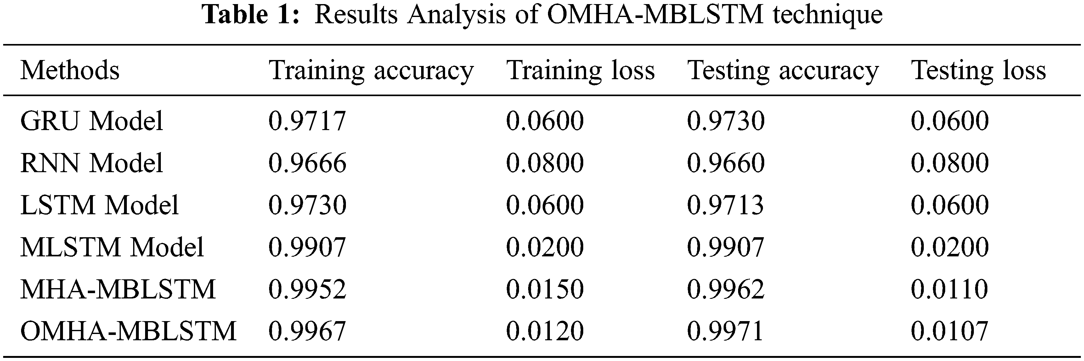
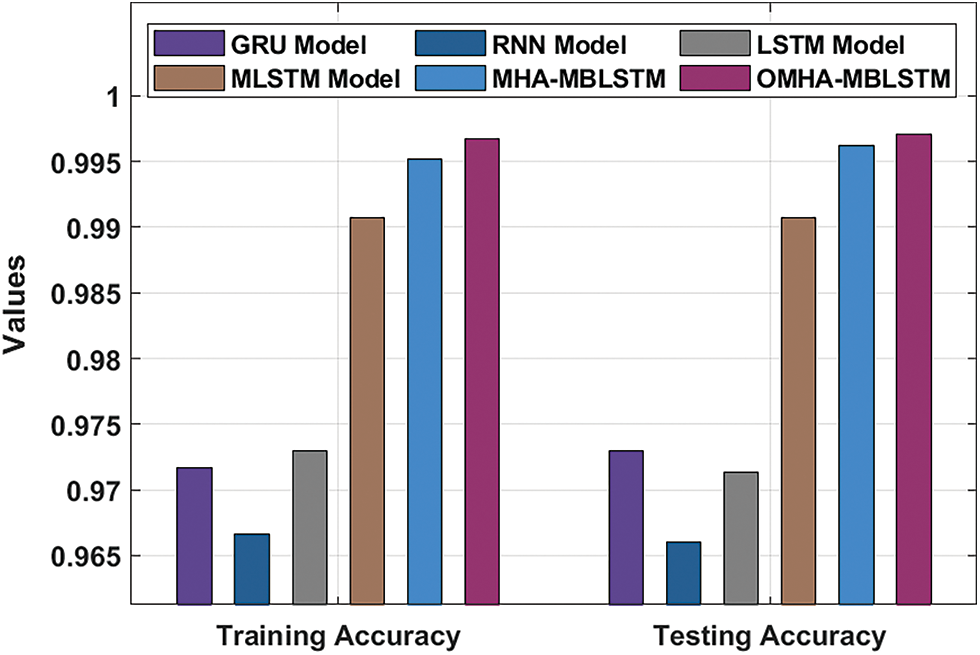
Figure 3: Training and testing accuracy analysis of OMHA-MBLSTM technique

Fig. 4 examines the comparative training loss and testing loss of the OMHA-MBLSTM technique. The figure reported that the RNN model has demonstrated worse performance poor with the maximum training loss and testing loss. At the same time, the GRU and LSTM models have tried to attain certainly reduced training loss and testing loss. Meanwhile, the MLSTM and MHA-BLSTM models have resulted in moderately reduced training loss and testing loss. However, the OMHA-MBLSTM technique has surpassed the other DL models with the least training loss and testing loss of 0.0120 and 0.0107 respectively.

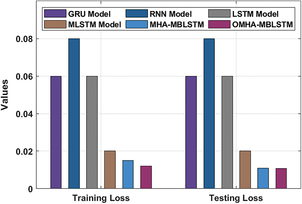
Figure 4: Training and testing loss analysis of OMHA-MBLSTM technique

Fig. 5 illustrates the ROC analysis of the MHA-MBLSTM model for the stability prediction of the smart grid. The results revealed that the MHA-MBLSTM technique can accomplish improved stability prediction outcomes with the increased ROC of 99.9221.

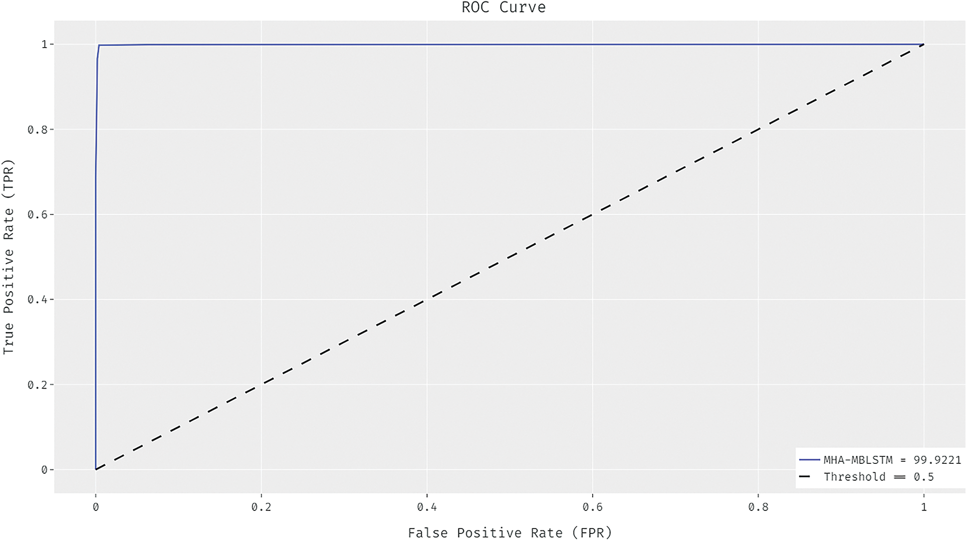
Figure 5: ROC analysis of MHA-MBLSTM technique

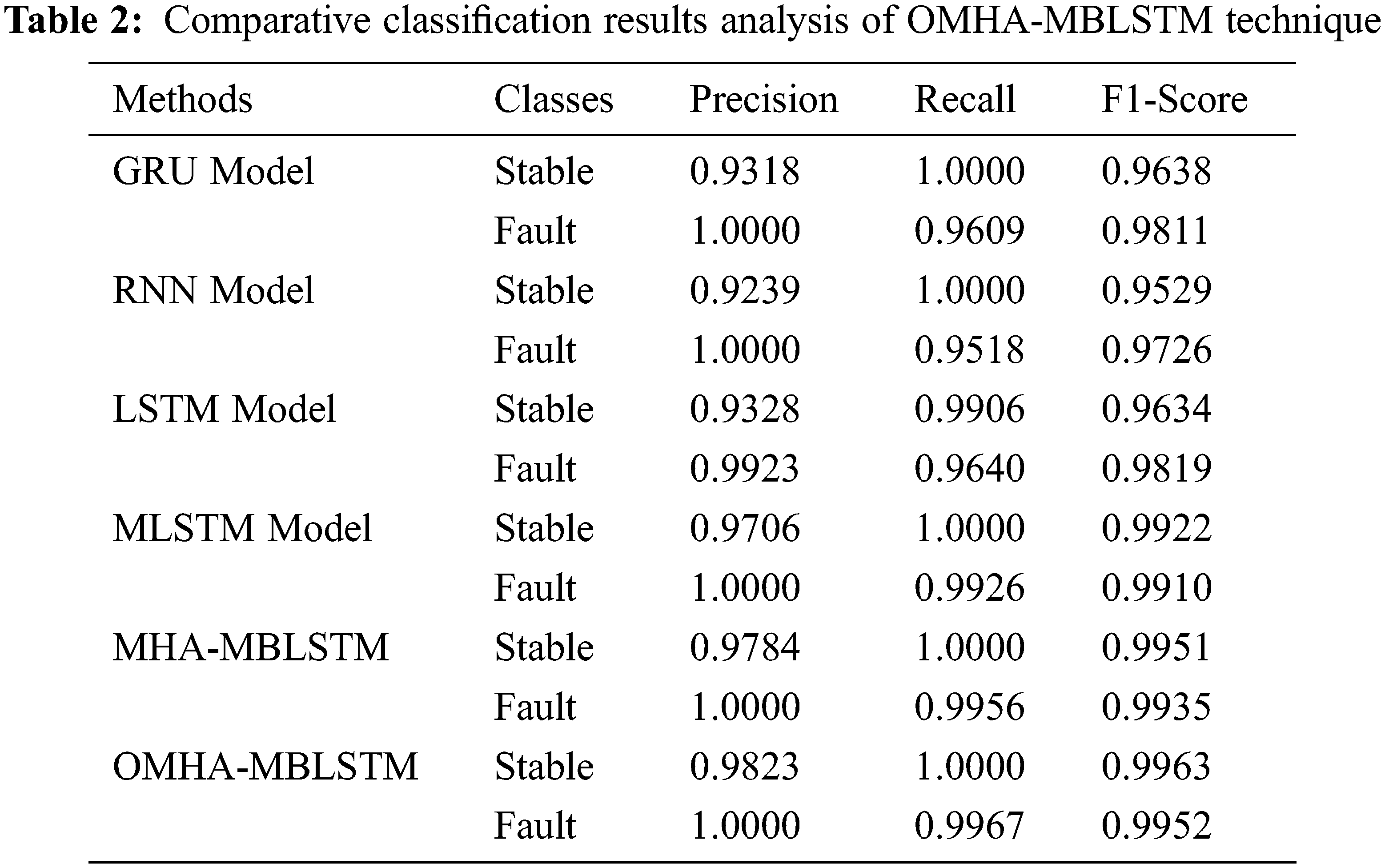
Fig. 6 exemplifies the ROC analysis of the OMHA-MBLSTM model for the stability prediction of the smart grid. The results discovered that the OMHA-MBLSTM technique has demonstrated better stability prediction outcomes with the maximum ROC of 99.9958. Tab. 2 offers a brief comparative result analysis [21] of the OMHA-MBLSTM technique. The results reported that the OMHA-MBLSTM technique has showcased enhanced outcomes over the other methods. For instance, the OMHA-MBLSTM technique has identified the instances into Stable class with the precn, recl, and F1score of 0.9823, 1.0000, and 0.9963 respectively. Moreover, the OMHA-MBLSTM technique has identified the instances into Fault class with the precn, recl, and F1score of 1.0000, 0.9967 and 0.9952 respectively.

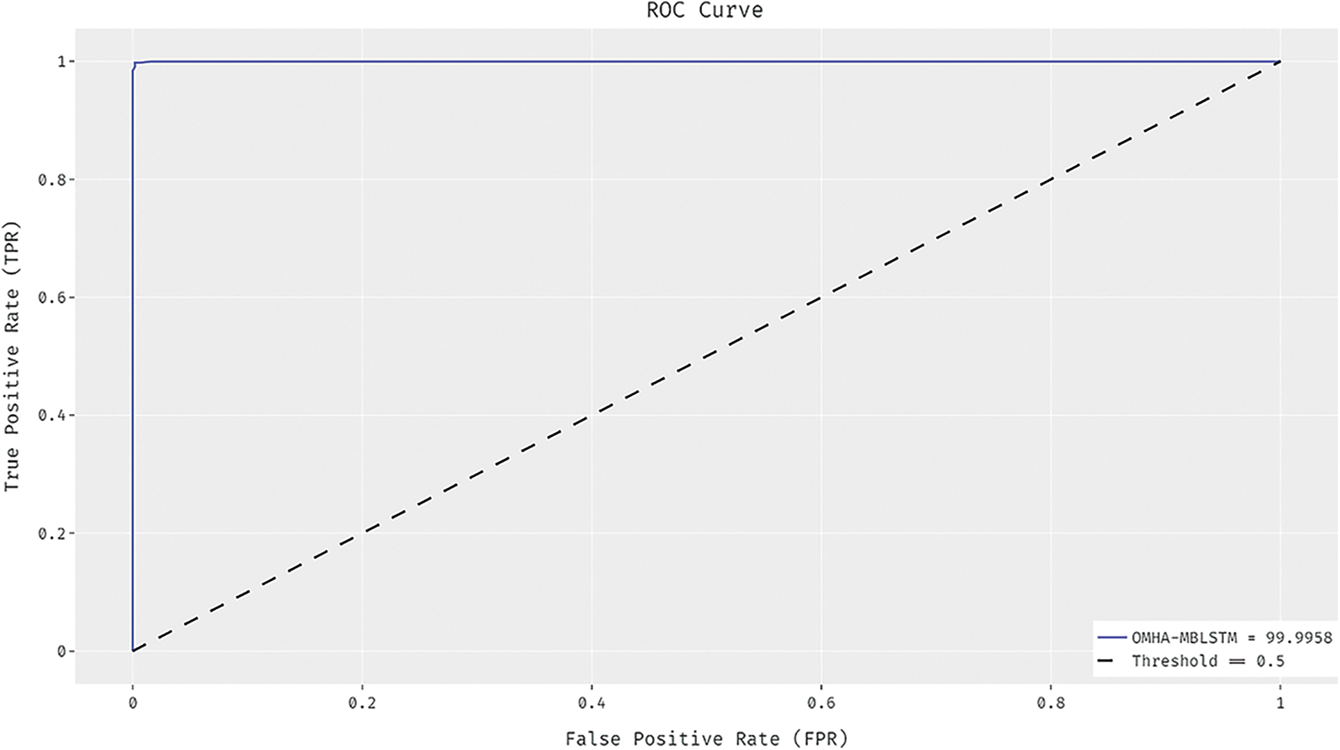
Figure 6: ROC analysis of OMHA-MBLSTM technique

Tab. 3 provides an average prediction result analysis of the OMHA-MBLSTM technique with recent methods [21]. Fig. 7 displays a brief precn analysis of the OMHA-MBLSTM technique with existing techniques. The results showcased that the GRU, RNN, and LSTM models have reached to least precn if 96.59%, 96.20%, and 96.26% respectively. Though the MLSTM and MHA-MBLSTM techniques have resulted in competitive precn of 98.53% and 98.92%, the OMHA-MBLSTM technique has demonstrated better outcome with the precn of 99.12%.

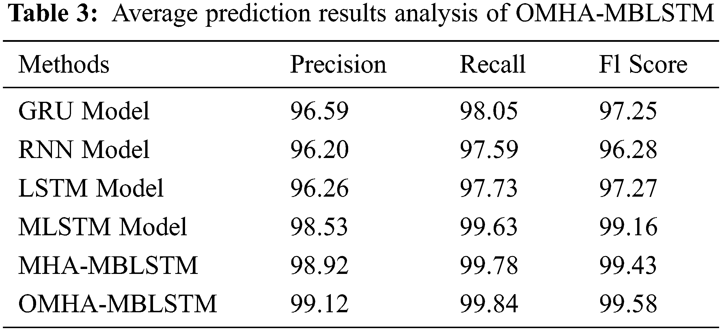
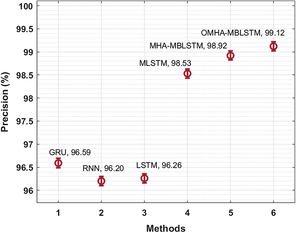
Figure 7: Comparative precn analysis of OMHA-MBLSTM technique

Fig. 8 offers a comprehensive recl analysis of the OMHA-MBLSTM technique with existing techniques. The figure revealed that the GRU, RNN, and LSTM models have obtained lower recl if 96.59%, 96.20%, and 96.26% respectively. Although the MLSTM and MHA-MBLSTM techniques have attained reasonable recl of 98.53% and 98.92%, the OMHA-MBLSTM technique has achieved improved outcome with the recl of 99.12%.

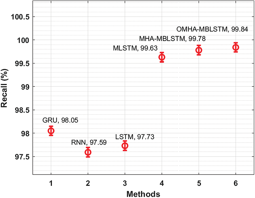
Figure 8: Comparative recl analysis of OMHA-MBLSTM technique

Finally, Fig. 9 reports an extensive F1score  analysis of the OMHA-MBLSTM technique with existing techniques. The results indicated that the GRU, RNN, and LSTM models have demonstrated ineffective F1score if 96.59%, 96.20%, and 96.26% respectively. Though the MLSTM and MHA-MBLSTM techniques have exhibited near optimal F1score of 98.53% and 98.92%, the OMHA-MBLSTM technique has demonstrated better outcome with the F1score of 99.12%. From the abovementioned results and discussion, it can be confirmed that the OMHA-MBLSTM technique has gained maximum stability prediction performance over the other techniques.

Figure 9: Comparative F1score analysis of OMHA-MBLSTM technique

4  Conclusion

In this study, an effective OMHA-MBLSTM technique has been developed to predict the stability level of the smart grids in the CPES environment. The proposed OMHA-MBLSTM technique involves three subprocesses such as min-max normalization based pre-processing, MBLSTM based prediction, and MHA based hyperparameter optimization. The design of MHA helps to appropriately elect the hyperparameters and it leads to enhanced predictive outcomes. For ensuring the improved performance of the OMHA-MBLSTM technique, a series of simulations were carried out and the results are inspected under several aspects. The experimental results pointed out the better outcomes of the OMHA-MBLSTM technique over the recent models. Therefore, the OMHA-MBLSTM technique can be used as an efficient tool for stability prediction in smart grids. In future, the predictive outcome can be improved by the utilization of hybrid DL models.

Acknowledgement: The authors would like to acknowledge the support provided by AlMaarefa University while conducting this research work.

Funding Statement: This research was supported by the Researchers Supporting Program (TUMA-Project-2021-27) Almaarefa University, Riyadh, Saudi Arabia. Taif University Researchers Supporting Project number (TURSP-2020/161), Taif University, Taif, Saudi Arabia.

Conflicts of Interest: The authors declare that they have no conflicts of interest to report regarding the present study.

References

 1.  I. Zografopoulos, J. Ospina, X. Liu and C. Konstantinou, “Cyber-physical energy systems security: Threat modeling, risk assessment, resources, metrics, and case studies,” IEEE Access, vol. 9, pp. 29775–29818, 2021. [Google Scholar]

 2.  C. Konstantinou and O. M. Anubi, “Resilient cyber-physical energy systems using prior information based on Gaussian process,” IEEE Transactions on Industrial Informatics, vol. 18, no. 3, pp. 2160–2168, 2022. [Google Scholar]

 3.  J. Ospina, I. Zografopoulos, X. Liu and C. Konstantinou, “DEMO: Trustworthy cyberphysical energy systems: Time-delay attacks in a real-time co-simulation environment,” in Proc. of the 2020 Joint Workshop on CPS&IoT Security and Privacy, Virtual Event USA, pp. 69–69, 2020. [Google Scholar]

 4.  R. Snijders, P. Pileggi, J. Broekhuijsen, J. Verriet, M. Wiering et al., “Machine learning for digital twins to predict responsiveness of cyber-physical energy systems,” in 2020 8th Workshop on Modeling and Simulation of Cyber-Physical Energy Systems, Sydney, Australia, pp. 1–6, 2020. [Google Scholar]

 5.  Y. Chen, S. Vinco, D. J. Pagliari, P. Montuschi, E. Macii et al., “Modeling and simulation of cyber-physical electrical energy systems with systemC-AMS,” IEEE Transactions on Sustainable Computing, vol. 5, no. 4, pp. 552–567, 2020. [Google Scholar]

 6.  C. Y. Lin, S. Zeadally, T. S. Chen and C. Y. Chang, “Enabling cyber physical systems with wireless sensor networking technologies,” International Journal of Distributed Sensor Networks, vol. 8, no. 5, pp. 489794, 2012. [Google Scholar]

 7.  M. L. Tuballa and M. L. Abundo, “A review of the development of smart grid technologies,” Renewable & Sustainable Energy Reviews, vol. 59, pp. 710–725, 2016. [Google Scholar]

 8.  K. Mahmud, A. K. Sahoo, E. Fernandez, P. Sanjeevikumar and J. B. H. Nielsen, “Computational tools for modeling and analysis of power generation and transmission systems of the smart grid,” IEEE Systems Journal, vol. 14, no. 3, pp. 3641–3652, 2020. [Google Scholar]

 9.  N. Kumar, S. Zeadally and J. J. P. C. Rodrigues, “Vehicular delay-tolerant networks for smart grid data management using mobile edge computing,” IEEE Communications Magazine, vol. 54, no. 10, pp. 60–66, 2016. [Google Scholar]

10. N. Bassamzadeh and R. Ghanem, “Multiscale stochastic prediction of electricity demand in smart grids using Bayesian networks,” Applied Energy, vol. 193, pp. 369–380, 2017. [Google Scholar]

11. J. Wei and G. J. Mendis, “A deep learning-based cyber-physical strategy to mitigate false data injection attack in smart grids,” in 2016 Joint Workshop on Cyber- Physical Security and Resilience in Smart Grids (CPSR-SG), Vienna, Austria, pp. 1–6, 2016. [Google Scholar]

12. A. Sargolzaei, C. D. Crane, A. Abbaspour and S. Noei, “A machine learning approach for fault detection in vehicular cyber-physical systems,” in 2016 15th IEEE Int. Conf. on Machine Learning and Applications (ICMLA), Anaheim, CA, USA, pp. 636–640s, 2016. [Google Scholar]

13. A. K. Bashir, S. Khan, B. Prabadevi, N. Deepa, W. S. Alnumay et al., “Comparative analysis of machine learning algorithms for prediction of smart grid stability,” International Transactions on Electrical Energy Systems, vol. 31, no. 9, pp. 1–23, 2021. [Google Scholar]

14. A. Jafari, F. Darbandi and H. Karimipour, “Instability prediction in smart cyber-physical grids using feedforward neural networks,” in 2020 IEEE Electric Power and Energy Conf. (EPEC), Edmonton, AB, Canada, pp. 1–6, 2020. [Google Scholar]

15. N. Tzanis, N. Andriopoulos, A. Magklaras, E. Mylonas, M. Birbas et al., “A hybrid cyber physical digital twin approach for smart grid fault prediction,” in 2020 IEEE Conf. on Industrial Cyberphysical Systems (ICPS), Tampere, Finland, pp. 393–397, 2020. [Google Scholar]

16. Q. A. A. Haija, A. A. Smadi and M. F. Allehyani, “Meticulously intelligent identification system for smart grid network stability to optimize risk management,” Energies, vol. 14, no. 21, pp. 6935, 2021. [Google Scholar]

17. V. K. Singh and M. Govindarasu, “A Cyber-physical anomaly detection for wide-area protection using machine learning,” IEEE Transactions on Smart Grid, vol. 12, no. 4, pp. 3514–3526, 2021. [Google Scholar]

18. T. Chen, R. Xu, Y. He and X. Wang, “Improving sentiment analysis via sentence type classification using BiLSTM-CRF and CNN,” Expert Systems with Applications, vol. 72, pp. 221–230, 2017. [Google Scholar]

19. S. Wang, Y. Zhu, W. Gao, M. Cao and M. Li, “Emotion-semantic-enhanced bidirectional lstm with multi-head attention mechanism for microblog sentiment analysis,” Information, vol. 11, no. 5, p. 280, 2020. [Google Scholar]

20. D. Oliva, S. E. Torres, S. Hinojosa, M. P. Cisneros, V. O. Enciso et al., “Opposition-based moth swarm algorithm,” Expert Systems with Applications, vol. 184, pp. 115481, 2021. [Google Scholar]

21. M. Alazab, S. Khan, S. S. R. Krishnan, Q. V. Pham, M. P. K. Reddy et al., “A multidirectional LSTM model for predicting the stability of a smart grid,” IEEE Access, vol. 8, pp. 85454–85463, 2020. [Google Scholar]

This work is licensed under a Creative Commons Attribution 4.0 International License, which permits unrestricted use, distribution, and reproduction in any medium, provided the original work is properly cited.