Computer Systems Science & Engineering DOI:10.32604/csse.2023.026744
Article

Efficient Object Detection and Classification Approach Using HTYOLOV4 and M2RFO-CNN

V. Arulalan* and Dhananjay Kumar

Department of Information Technology, Anna University, MIT Campus, Chennai, 600044, India
*Corresponding Author: V. Arulalan. Email: arulalan@mitindia.edu
Received: 04 January 2022; Accepted: 10 March 2022

Abstract: Object detection and classification are the trending research topics in the field of computer vision because of their applications like visual surveillance. However, the vision-based objects detection and classification methods still suffer from detecting smaller objects and dense objects in the complex dynamic environment with high accuracy and precision. The present paper proposes a novel enhanced method to detect and classify objects using Hyperbolic Tangent based You Only Look Once V4 with a Modified Manta-Ray Foraging Optimization-based Convolution Neural Network. Initially, in the pre-processing, the video data was converted into image sequences and Polynomial Adaptive Edge was applied to preserve the Algorithm method for image resizing and noise removal. The noiseless resized image sequences contrast was enhanced using Contrast Limited Adaptive Edge Preserving Algorithm. And, with the contrast-enhanced image sequences, the Hyperbolic Tangent based You Only Look Once V4 was trained for object detection. Additionally, to detect smaller objects with high accuracy, Grasp configuration was observed for every detected object. Finally, the Modified Manta-Ray Foraging Optimization-based Convolution Neural Network method was carried out for the detection and the classification of objects. Comparative experiments were conducted on various benchmark datasets and methods that showed improved accurate detection and classification results.

Keywords: Object detection; hyperbolic tangent YOLO; manta-ray foraging; object classification

1  Introduction

Object Detection (OD) is a vital aspect of image processing, in addition to machine vision, which is extensively utilized [1] in various fields like robot navigation, industrial detection, intelligent video surveillance, and aerospace [2]. Particularly, OD and tracking are considered to be the fundamental applications of remote sensing [3]. In which, OD is carried out in aerial video surveillance using unmanned vehicles [4,5]. Chiefly, finding the objects belonging to particular classes and their respective locations on the images or videos is the task of the OD [6]. Usually, the machines consume more time for training as well as testing to detect the objects in a video [7]. Nevertheless, it is hard for the machines to distinguish the objects. For that, knowledge-building process is required with an effectual algorithm [8]. A significant improvement can well be seen on the OD algorithms latterly [9]. In computer vision, there are two major issues, viz. object-localization and object classification in a video or image [10,11]. The major purpose of the Object localization is to locate objects through drawing a Bounding Box (BB) exactly around the object [12]. And, the automatic classification of objects stands as a crucial issue and has widespread applications. Traditionally, in computer vision system, detection was initially done for the object and disparate algorithms are combined to classify them. Then, those algorithms are centered on high-quality images [13].

The quality of the extracted features and the robustness of the classifiers play a major role in the OD and classifications performance [14]. Generally, to find the object-of-interest on an image, OD utilizes distinctive shape patterns as evidence [15]. For describing an object on an image, a crucial role is played by the selection as well as extraction of distinct key points in object recognition applications [16]. OD is considered to be a crucial and an active field in Information and Technology which prompted the curiosity among many researchers. Unlike the images, videos have temporal information [17]. For an additional processing, every frame is captured and combined as one during video processing [18]. It is an extremely vital and challenging task to detect and track moving objects or targets on real-time video surveillance [19]. On account of the augmented demand for intelligent surveillance systems, object tracking has emerged as a meticulous research topic. Object detection and tracking are extensively utilized in the event of crowd flow estimation, behavior understanding, and human-computer interaction [20].

Complexities in computation and accuracy are the other major issues in the existing techniques meant for OD. In the present study, an efficient OD and classification system were proposed utilizing Hyperbolic Tangent based You Only Look Once V4 (HTYOLOV4), together with with the Modified Manta-Ray Foraging Optimization-based Convolution Neural Network (M2RFO-CNN).

The organization of the present paper is as follows. Firstly, Section 1 introduces OD and its various aspects and Section 2 elucidates the related review of the existing methods regarding object detection. Then, the proposed OD and the classification technique using HTYOLOV4 and M2RFO-CNN are illustrated in Section 3. And, in Section 4, the proposed method’s performance is discussed and compared with the existing methods. Finally, in Section 5, the conclusions drawn from the results of the present study is given with the suggestions for further enhancements that can be made in the future.

2  Related Works

OD with Binary Classifiers is a two-level technique which is centered on Deep Learning (DL) that overcomes the issue of identifying smaller objects like weapons in surveillance video [21]. In the first level, the candidate regions were chosen from the input frames and those proposals were analyzed in the second level. Centered upon a CNN with One-vs.-All or One-vs.-One, a binarization technique was also applied. And, concerning the baseline multi-class detection, the total false positives were reduced. The preprocessing strategies to filter out the noisy instances decreased the detection accuracy of the CNN.

A modified YOLOv1 with an improved Neural Network for objection detection was proposed [22] and the Loss Function (LF) of the YOLOv1 was modified. The margin style was replaced with the proportion style. Next, a spatial pyramid Pooling Layer was added. An inception design was added with a convolution kernel which cut the total weight parameters of the layers. The performance attained was found to be better, nevertheless, for smaller objects detection, the technique was not appropriate.

A recommended multiple-scaled deformable convolutional OD network was introduced to handle the challenges that were faced by some detectors [23]. For obtaining multi-scaled features, deep convolutional networks were used. For overcoming geometric transformations, deformable convolutional structures were added. In order to apply the last object recognition, as well as region regress, the multiple-scaled features were fused by upsampling. The accuracy of detecting smaller target objects with geometrics deformation was also improved. Significant improvements on the trade-off between speed and accuracy were also seen. However, the technique did not help detecting objects on videos.

Instantaneous OD for videos centered on the YOLO network was discussed [24]. The quick YOLO model was trained for OD to attain the object information. By replacing a smaller convolution operation with the original convolution operation, the YOLO was ameliorated upon the Google Inception Net (GoogLeNet) architecture. It reduced the total parameters and also reduce the time for OD in videos. This technique performed better contrasted with the original YOLO and the other baseline methods. A high computation load in addition to low detection speed was found.

The hybrid deep-learning model is called Faster-RCNN, along with Mask-RCNN [25] model encompassing two major portions. The region proposal network is the first portion that was utilized to generate a list of region proposals intended for an input image. Classification helped in the identification of the ROI of the object or no object. Then, the ROI PL accepted the chosen region proposals as the input. Additionally, it classified the class and refined the bounding box aimed at the object which provided the output image. The overhead view object was detected together with the classified bounding box. The second approach aimed at overhead view object detection was designed on Mask R-CNN. The model took care of locating the exact pixels of every object, together with the detected BB. Those algorithms encompassed with stronger discriminative power intended for multiple OD. Nevertheless, the method’s accuracy was a lower enhancement.

3  Proposed Object Detection Methodology

An OD task for specific crowded macro-scene, as well as the microcosm, is the Small Object Detection (SOD) with larger objects. OD involves two specific tasks, viz. to assess the object locations and the BB for additional applications like object classification and recognition. Utilizing modern DL models, useful detectors can be designed well to overcome such issues when the target objects are of distinct sizes, colors, shapes, and textures. Nevertheless, when the target objects are smaller, the task can be more complex. A novel approach for OD and classification is proposed utilizing Hyperbolic Tangent based You Only Look Once V4 (HTYOLOV4), along with Modified Manta-Ray Foraging Optimization-based Convolution Neural Network (M2RFO-CNN).

Initially, the video data are converted into image sequences. In pre-processing steps, resizing and noise removal are done using Polynomial Adaptive Edge preserving Algorithm (PAEPA). To enhance contrast for the resized noiseless image sequences, Contrast Limited Adaptive Edge Preserving Algorithm (CLAHE) was applied after preprocessing. Subsequently, HTYOLOV4 was trained with the contrast-enhanced image sequences for object detection. All the objects were detected at the end of this step with their bounding box and the loss was calculated. Hence, to enhance the accuracy for detecting the small objects, Grasp configuration was considered and checked with the threshold value to attain the smaller and bigger objects. Finally, the M2RFO-CNN algorithm executed the object detection and classification step. The proposed system architecture is exhibited in Fig. 1.

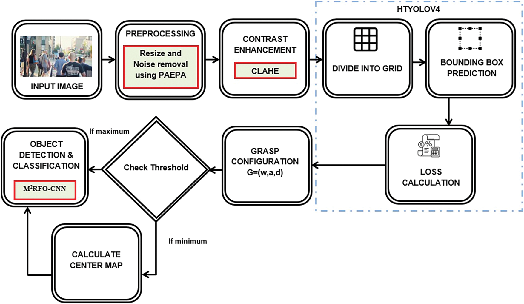
Figure 1: System architecture of proposed methodology

3.1 Preprocessing

At the initial stage, the video data were converted into several frames. In the pre-processing, PAEPA removes the noise present on the input frame images. For improving the clarity, image resizing was done before noise removal. Generally, the pixel information gets changed and the image's clarity also becomes low while augmenting the image’s size. The polynomial interpolation function was utilized for resolving this issue and making the image clear. By generating the equivalent approximation of pixel intensities concerning the surrounding pixel values, the interpolation function enhanced the image’s clarity. The number frames are signified as,

Inputvideo:Qi→If(m) (1)

Ifi(m)={If1(m),If2(m),If3(m),.............Ifn(m)} (2)

where, Ifi(m) signifies the sequence frameset, fi signifies the n - number of frames, and Qi implies the input video to attain the total frames.

Step 1: The resizing can well be done as,

Ifi(m)rs⟶resizingIfi(m)ipt (3)

where, Imrs signifies the resized image and Imipt implies the input image to be resized. For ameliorating the image’s clarity, the resized image is interpolated by the polynomial interpolation technique. Therefore, the interpolating polynomials U(ϕ) for the image can well be attained as,

U(ϕ)=αo+α1ϕ1+α2ϕ2+......+αnϕn (4)

wherein, n signifies the degree of the polynomial and α0,....αn signifies the coefficients. By taking an average of surrounding known pixel values of the unknown pixel, the interpolated pixel values are computed for obtaining the interpolated image.

Step 2: The interpolated image for noise removal is expressed as,

Ifi(m)=Ifi(m)ip+D (5)

wherein, Ifi(m)ip signifies the interpolated image with polynomials and Ifi(m) implies the observed image with corrupted noise D . The image is partitioned into several blocks at the time of noise removal. Every block is applied to Discrete Wavelet Transform (DWT). Several coefficients from DWT are attained as the edge information. The DWT co-efficient can well be attained as,

C=T(Bn(Ifi(m))) (6)

wherein, T signifies the DWT function, Bn denotes the partitioned block of the input image Im , C denotes the wavelet coefficients in a,b directions.

Step 3: Concentrated on their sub-bands, the threshold is estimated to suppress noise. The threshold can well be estimated as,

τt=med|Cab|0.6745×1max(Δg2−Δnoise2,0) (7)

Δg=1L∑a,b=1LCab (8)

wherein, Δnoise signifies the noise variance, L implies the total wavelet coefficients Cab , τt implies the estimated threshold, med implies the median factor used for estimating noise variance as of diagonal detail.

Step 4: For calculating the threshold, the shrinkage rule is utilized. Thus, smaller threshold values are possessed by active edges. Thresholding is applied for the wavelet coefficients by the shrinkage rule, which is shown below,

τCab=β×τt (9)

wherein, β signifies the shrinkage function τCab implies the thresholded coefficients.

Step 5: Lastly, for reconstructing the noise-removed image, the inverse wavelet transforms for the thresholded coefficients are done. The inverse wavelet transform can well be expressed as,

Im∧=T−1(τCab) (10)

wherein, Im∧ denotes the denoised image, T−1(∙) denotes the inverse wavelet transform.

3.2 Contrast Enhancement

The CLAHE enhanced the contrast of the noise-removed image I^m . Here, the inputted image I^m was split into several sub-regions. For every sub-region, the histogram was calculated and the histograms were clipped. In clipping, utilizing the clip limit, the pixels were equally distributed to every gray level. The clip limit can well be attained as,

Limclip=χ(x,y)Tgl(1+φφmax(hmax−1)) (11)

wherein, Limclip signifies the clip limit, χ(x,y) signifies the total pixels in x,y the dimension of the sub-region, Tgl implies the total gray levels, Ccl signifies the normalized clip limits, φ signifies the factor ranges as of to φmax , and hmax implies the maximum limit of the histogram. The clipped histograms are equally redistributed. The transformation function is utilized for interpolation after the histogram is clipped as well as redistributed. The transformation function is stated as,

ℑ=Tgl−1χ(x,y)∑l=0LCDf(l) (12)

wherein, CDf(l) signifies the cumulative distribution function scaled by (Tgl−1) and is utilized for histogram equalization of l regions, ℑ implies the transformation function of gray-scale mapping. Lastly, to attain the enhanced image Imenh , the split regions are incorporated.

3.3 Object Detection Using HTYOLOV4

The HTYOLOV4 was trained Imenh for OD after contrast enhancement. YOLOV4 is considered to be the extended edition of YOLOV3. Backbones, neck, as well as heads, are the 3 important stages. The pre-trained NN is regarded as the backbone, which extracts the necessary features as of the input image. Numerous top-down, as well as bottom-up paths, was encompassed by the neck for collecting Feature Maps (FM) as of disparate stages. The classes and bounding box of objects were predicted by the head. The input images were split into grids in the prediction process. Inaccurate detection of objects on the image can well result if the grid levels are larger. To resolve this issue, the Hyperbolic Tangent Kernel function reduced the grid levels, which brings accurate bounding box prediction as well as reduced Loss Function. Thus, the proposed technique is labeled HTYOLOV4. The Hyperbolic Tangent Kernel function split the input images into a grid of manifold cells. The HT is stated as,

HT(Imenh)=tanh⁡(β(u.v)+k) (13)

wherein, β and k are the slope and intercept constant also known as the adjustable parameters, (u.v) implies the dot product betwixt the points, β has the common value as (1/d), d signifies the m×m dimension of every grid. For determining whether there is an object in the grid or not, the object’s probability was computed for every grid. For every grid, the outputs say bounding box coordinates along with confidence score are attained if the grid encompasses an object. The Fig. 2 exhibits the dimensions utilized for the bounding box (BB) prediction.

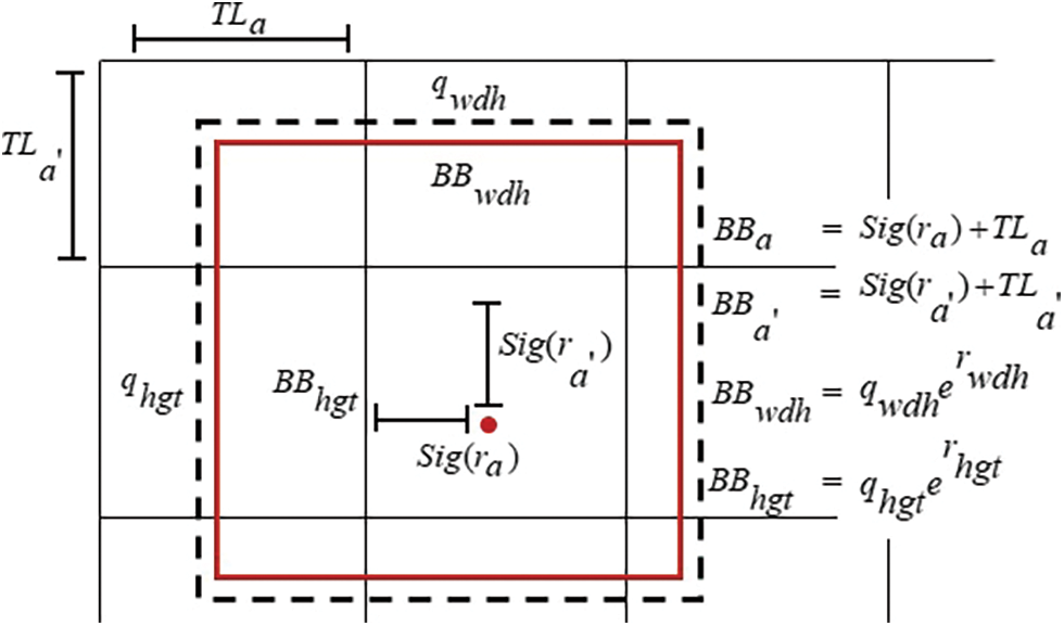
Figure 2: Bounding box with coordinates and location

The BB coordinates are expressed as,

BBa=sig(ra)+TLa (14)

BBa′=sig(ra′)+TLa′ (15)

BBwdh=qwdherwdh (16)

BBhgt=qhgterhgt (17)

where, BBa and BBa′ signify the center coordinates of the box, BBwdh and BBhgt imply the width, in addition to the height of the box, ra , ra′ , rwdh and signify the network outputs, (TLa,TLa′) imply the top-left coordinates of the grid, (qwdh,qhgt) imply the dimensions of BB priors termed anchors, sig implies the sigmoid function.

The confidence score rendered the probability of encompassing an object in the BB. For ignoring boxes with lower object probability and BB with the highest shared area in a process termed non-max suppression, the confidence score can well be utilized. The probability value concerning the object’s class is computed as,

P=P(Ciobj)∗P(obj)∗IoU (18)

IoU=BBP∩BBGTBBP∪BBGT (19)

where, P(Ciobj) signifies the probability of object that belongs to a category Ci inside the box, P(obj) implies the probability of identifying the center point of the object obj on the grid, BBP signifies the predicted box, together with BBGT signifies reference BB, Intersection over Union (IoU). Yet, there might be many overlapping boxes for detection even after the filtering positioned on the score values was performed. For removing manifold detections on the same image, Non-Maxima Suppression (NMS) was carried out. The large overlap boxes with the chosen box were mitigated by employing NMS. Only the best boxes were left with the object’s position, BB’s confidence level, along the class probability. After that, centered on three sorts of error information, the loss function ρloss is computed as,

ρloss=∑(e(BBa,BBa′)+eIoU+eCi) (20)

where, e(BBa,BBa′) signifies the position error, eIoU implies the error in confidence level, together with eCi signifies the errors of class probability.

3.4 Grasp Configuration

After object detection, this step is used to improve the accuracy of detecting smaller objects. Width, angle, as well as depth, which are the grasp configuration, are gauged for every BB with detected objects. The grasp configuration of the detected objects G is written as,

G={hgt,wdh,Ang} (21)

where, hgt signifies the BB’s height, wdh is the BB’s width, together with Ang signifies the angle that renders the BB’s direction concerning the horizontal axis. Next, the values attained in the grasp configuration are checked with the threshold value.

Dn={Dn(big)if(G>λ)Dn(small)cmif(G<λ) (22)

If the threshold value λ is exceeded by the extracted values, it is deemed as the big object Dn(big) and is moved to the OD as well as recognition step; otherwise, the object is regarded as a smaller object Dn(small)cm . The center map for the detected object is computed when the object is detected as small. The center map of the box made it easy to match the box, which contains the middle of the object to a grid cell. Next, those center map object is rendered to the OD together with the recognition step.

3.5 Object Detection and Classification

M2RFO-CNN takes care of the object detection and classification task. For ameliorating the accuracy of detecting even smaller objects, every detected image Dn was trained again utilizing this algorithm. An artificial neural network that is extensively utilized for objection detection in CNN. For differentiating one from the other, the image input was taken and assigned the learnable weights to the objects on the image. The detection quality utilizing CNN was ascertained through the LF that renders the deviation betwixt the predicted output and true labels. The prediction performance was affected once the Loss Function renders maximum. The weight value generated in every node of CNN requires to be optimized for reducing the LF together with the training time and improving the model’s accuracy.

The M2RFO is employed for optimizing the CNN’s weights. In MRFO, only particular ranges were concentrated for the best solution generation in cyclone foraging, which makes the Manta Ray (MR) not capture the optimal solution available past the range. The Gradient Descent method generated the lower and the upper boundaries of the problem space in MRFOA for solving this issue. M2RFO-CNN was presented with this modification. The M2RFO-CNN structure is shown in Fig. 3.

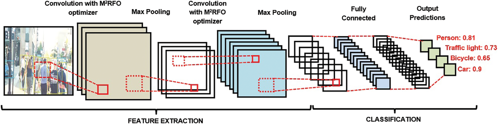
Figure 3: Structure of M2RFO-CNN classifier

3.5.1 Convolution Layer (CL)

Initially, the input data goes through convolution operation in the CL and outputted the FM. The convolution kernels are utilized by the layer that slides over every position of the FM aimed at convolution operation. The kernels predict at every position. The CL’s output is implied as,

ξL(H)=Dn∗ϑ(δ(k)) (23)

where, ξL(H) signifies convolutional layer’s output, Dn implies the detected objects, ϑ(∙) implies the non-linear activation function, along with δ(k) signifies the weight vector of every input node.

3.5.2 Pooling Layer

For reducing the spatial size of output that was attained at the CL, the PL is used. The CL lessens the size through extracting the utmost dominant features utilizing the max-pooling function as of the chosen region. The PL’s output is expressed as,

ξL(H)=υMAX(ξL(H)) (24)

where, ξL(H) signifies the PL output and υMAX implies the max-pooling function.

3.5.3 Fully Connected Layer

The pooled output at the PL is flattened as well as inputted to the FCL. The computation is done for every layer present at the FCL as,

ξfc=ϑl(∑l=1nξL(H)δ(k)+Bl) (25)

where, Bl signifies the bias vector, ξfc implies the FCL’s output, n implies the number of layers, and ϑl signifies the softmax activation functions. The last softmax layer classifies the objects as labels after passing through the FCL. Next, the LF is evaluated as,

LF=∑(κtar−κobs)2 (26)

where, κtar and κobs signify the target as well as observed values. When the target value is equivalent to the observed value, the proposed model falls into precise prediction; in addition, no optimization is required.

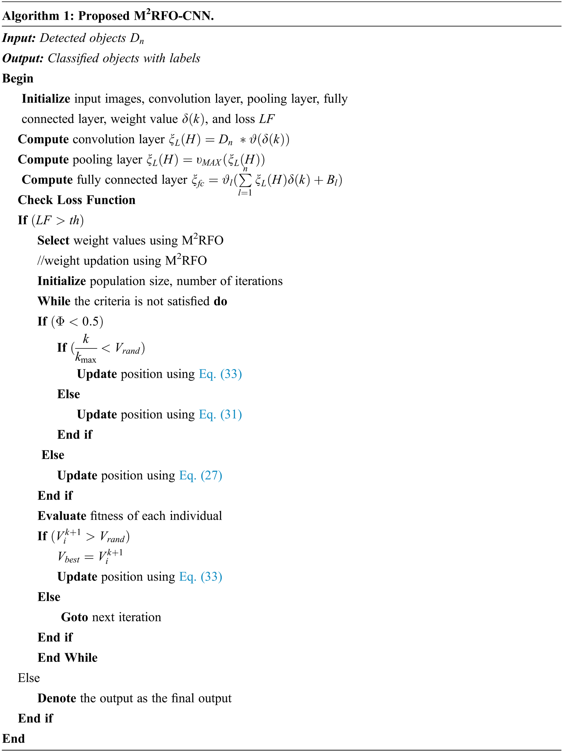
On the contrary, the optimization of weight values is needed for choosing the optimum weight values if the target values are not equivalent to the observed values. Here, the M2RFO was utilized for the optimization. The M2RFO-CNN algorithm is exhibited in Algo. 1.

MRFO is enthused by the foraging behavior of MR. It is a meta-heuristic algorithm. Chain, cyclone, and somersault foraging are the three foraging behaviors of the MR to seize their prey.

3.5.4 Chain Foraging

The best solution was detected by the MR (i.e.,) the highest concentration of plankton that the MR wants to devour. The populace of MR (i.e., the random weight values) formed a foraging chain once the best solution was found. Each individual moves in the direction of the food. Each individual carries out the position updation during this process. The chain foraging can well be expressed as,

Vik+1={Vik+Φ(Vbestk−Vik)+Ω(Vbestk−Vik)i=1Vik+Φ(Vi−1k−Vik)+Ω(Vbestk−Vik)i=2,3,4,.....M (27)

Ω=2Φ|logΦ|0.5 (28)

where, Vik signifies the position of ith individual at k , Vbestk implies the best solution at k , Φ∈[0,1] signifies an arbitrary vector, Ω implies the weighting coefficient, together with M , implies the population’s size.

3.5.5 Cyclone Foraging

Here, the MR forms a line and move in the directions of the food in the shape termed spiral when the plankton patch position is recognized. Every individual follows the MR swimming in front of it during spiral swimming. Therefore, the movement in spiral shape is stated as,

vik+1=vbest+Φ(vi−1k−vik)+eaxcos2πx(vbest−vik) (29)

yik+1=ybest+Φ(yi−1k−yik)+eaxcos2πx(ybest−yik) (30)

Exploitation and exploration are the stages encompassed in cyclone foraging. The reference position is chosen as the current best position on the exploitation stage. The cyclone foraging on exploitation is expressed as,

Vik+1={Vbest+Φ(Vbestk−Vik)+Θ(Vbestk−Vik)i=1Vbest+Φ(Vi−1k−Vik)+Θ(Vbestk−Vik)i=2,3,4,.....M (31)

Θ=2eΦ(kmax−(k+1))kmax.sin⁡(2πΦ) (32)

where, Θ signifies the weighting coefficient. Next, every individual is forced to search for a new position as of the current best one in the exploration phase. The reference position is assigned to each individual, which is randomly generated. The global search on exploration is written as,

Vik+1={Vrand+Φ(Vrandk−Vik)+Θ(Vrandk−Vik)i=1Vrand+Φ(Vi−1k−Vik)+Θ(Vrandk−Vik)i=2,3,4,.....M (33)

Vrand=Llow+Φ.∇(Lup−Llow) (34)

where, Vrand signifies the randomly generated reference position, Llow , Lup imply the upper as well as lower limits of every dimension in the search space generated utilizing the gradient descent method ∇ . For generating the upper and lower boundaries, the gradient descent method is utilized, which is written as,

ϖj=ϖj−1+Brd∇(Lup,Llow)dϖj (35)

where, Br signifies the learning rate, d∇dϖj(∙) implies the derivative of the performance function, ϖj signifies the change in limits for the total iterations. The exploitation and exploration phases are balanced utilizing kkmax ratio where, kmax is the maximal number of iterations. The MR can switch to the chain and cyclone foraging centered on the arbitrary number.

3.5.6 Somersault Foraging

Here, the food is regarded as a hub. Each individual turns over to the new position by moving forward and backward around the hub. Here, the MR updated its position around the best solution. Therefore, the somersault foraging can well be expressed as,

Vik+1=Vik+G.Φ(Vbest−Vi)i=1,2,3,......M (36)

where, G signifies the somersault factor. Here, every individual moved around the current position and the best solution. Every individual came near the optimal solution gradually as the distance betwixt the current and best position and the gamut of somersault foraging was lessened. Until the stopping criteria are met, the updation processes are performed. Concurrently, centered on the LF, the fitness is estimated for every individual’s best solution. Like this, the weight values were optimized. Lastly, the objects with labels were categorized by the classifier.

4  Results and Discussion

In this section, the performance measure of the proposed OD model is discussed, along with the experimental results.

4.1 Database Description

Caltech Pedestrian and PASCAL Visual Object Collection (VOC) datasets were used for performance analysis. These datasets roughly consisted of ten hours of 640 x 480 30 Hz video that was taken as of a vehicle moving in a regular traffic in an urban environment. Around 250,000 frames with 350,000 bounding boxes as well as 2300 unique pedestrians were annotated. Training, validation, private testing set are the three subsets of the PASCAL VOC dataset. Sample images of the dataset and further processing of the images are shown in Fig. 4. The Fig. 4a shows the input image of the dataset, Fig. 4b shows the preprocessed image by using the PAEPA algorithm, Fig. 4c shows the enhanced image by employing the CLAHE method, and then, the classified images are shown in Fig. 4d.

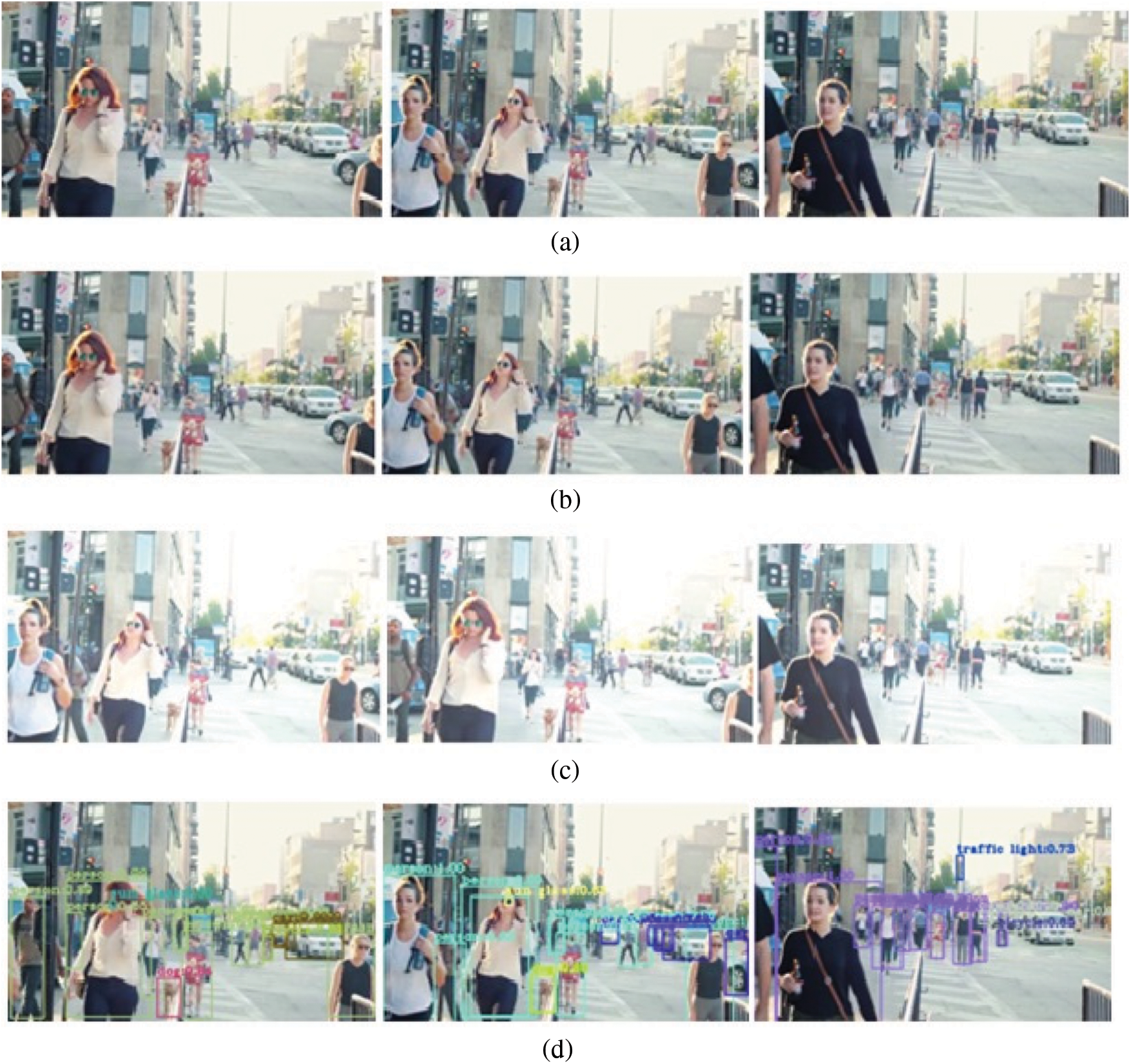
Figure 4: Sample images (a) input image, (b) preprocessed image, (c) contrast-enhanced image, (d) classified image

4.2 Performance Analysis

The analysis of the proposed and existing methods performance concerning sensitivity, specificity together with accuracy is exhibited in Tab. 1.

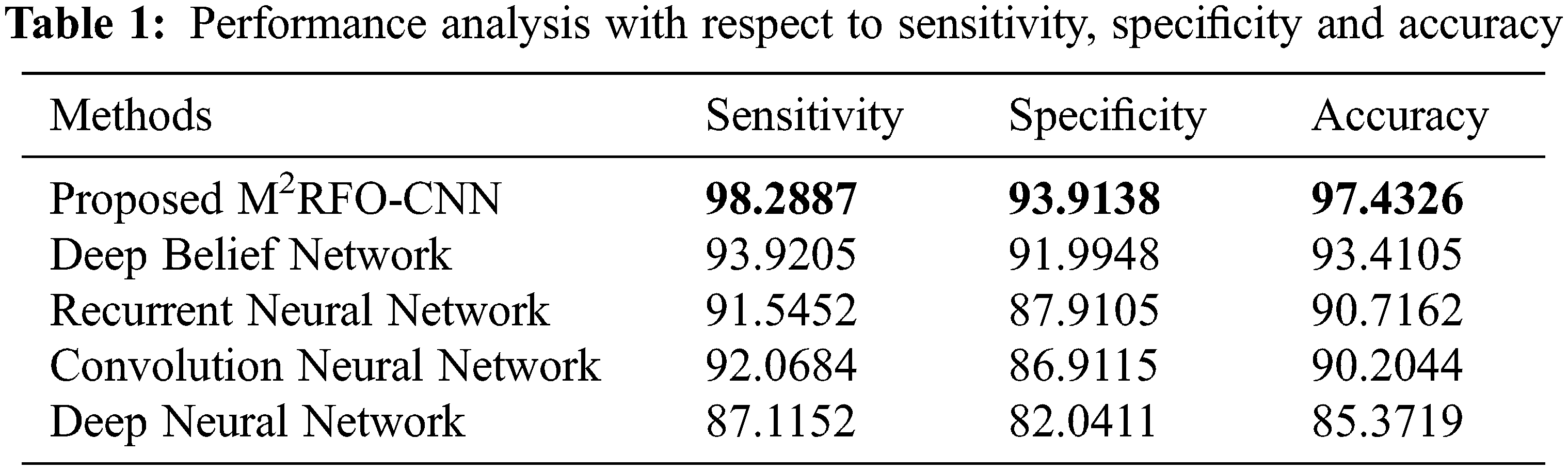
Sensitivity evaluates a model’s capability to predict the true positives of every available category. A model’s capability to envisage the true negatives of every available category was evaluated by specificity. Accuracy stands as the degree of closeness to the true value. Overall, it was revealed as of the performance outcomes concerning the sensitivity, specificity along with accuracy that the proposed methodology detects objects were found to be high. Likewise, Precision, Recall, F-Measure, Negative Prediction Value (NPV), and Matthews Correlation Coefficient (MCC) of the proposed model and the existing models namely Deep Belief Network (DBN), Recurrent Neural Network (RNN), Convolution Neural Network (CNN) together with Deep Neural Network (DNN) are compared is shown in Tab. 2.

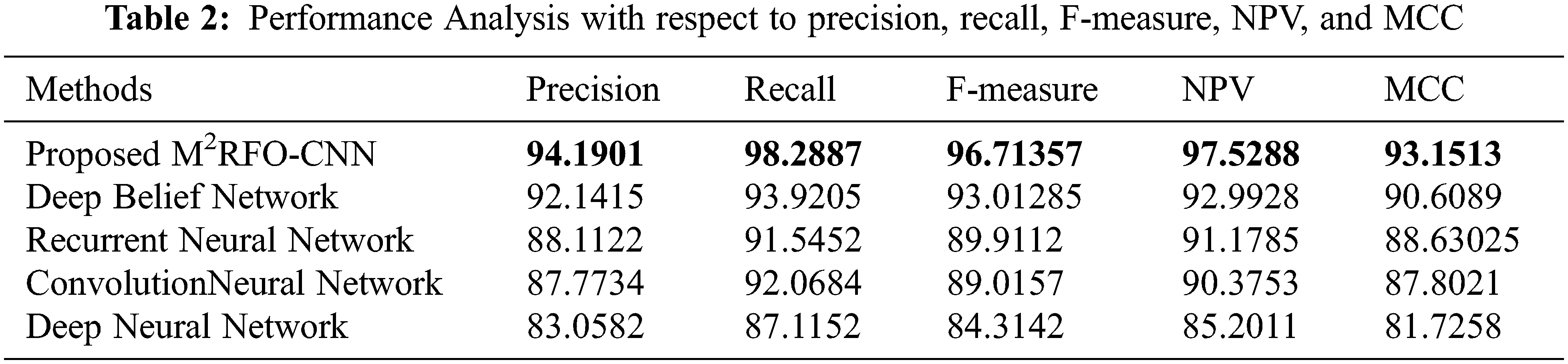
The total predictions that are a member of the corresponding class were quantified by the Precision metric. The total class predictions made out of every example in the dataset were defined as recall. The F-measure metric is the merger of the precision and the recall metrics. Compared to all the other prevailing techniques, the proposed work offered a better precision level. However, the recall and F-measure values of prevailing methods render comparatively lower performance. The proposed methodology attained a 97.5288 NPV value, which was found to be higher when weighed against the prevailing methods. Likewise, compared to prevailing methods, the proposed method attained a better MCC value. Hence, concerning all metrics, greater performance was attained by the proposed work. Concerning False Positive Rate (FPR), False Negative Rate (FNR), and False Rejection Rate (FRR) of the proposed and existing methods performances are examined in Tab. 3.

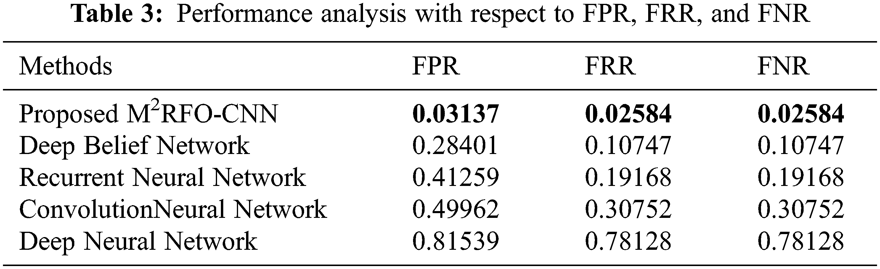
The Tab. 3 analyses the performance of the proposed and existing methods in terms of FPR, FRR, and FNR. These values were considered to contribute to the false prediction. The probability of wrongly rejecting the null hypothesis was termed false-positive rate. The percentage of identification instances where the identified objects are wrongly rejected is called FRR. An outcome wherein the negative class was incorrectly predicted by the model called the FNR. It has ignored the false prediction by attaining FPR, FNR, and FRR values closest to 0. On examining the above-given table, the false prediction has been ignored by the proposed method via attaining FPR, FNR, and FRR values closest to a minimum. Additionally, the FPR, FRR, and FNR values were possessed by the DBN, RNN, and CNN methods, which were found to be higher when contrasted to the proposed work. When weighed against the prevailing methods, lesser values were attained by the proposed work for FNR, FPR, and FRR. Therefore, the analysis deduces that objects were detected more effectively by the method when contrasted to the existent methods.

5  Conclusion

In present study, an efficient approach for object detection and classification method was proposed utilizing HTYOLOV4 and M2RFO-CNN. The proposed approach shows improved detection performance regarding the precision, recall, accuracy, F-Measure, sensitivity, specificity, NPV, MCC, FNR, FRR, and FPR. The frame sequences were enhanced by Polynomial Adaptive Edge preserving Algorithm, then, the HTYOLOV4 was trained with the contrast-enhanced frames. Also, Grasp configuration was employed for detecting smaller objects with higher accuracy. The proposed method was evaluated over various benchmark datasets like Caltech Pedestrian and PASCAL VOC datasets, and compared with the prevailing techniques to examine the efficiency of the proposed method. The M2RFO-CNN attains 97.4326 accuracies high on the performance analysis. The analysis proved that the proposed scheme showed improved efficiency for detection and classification. In the future, more advanced algorithms can be included for achieving higher performance.

Funding Statement: The authors received no specific funding for this study.

Conflicts of Interest: The authors declare that they have no conflicts of interest to report regarding the present study.

References

 1.  J. Yuan, H. C. Xiong, Y. Xiao, W. Guan, M. Wang et al., “Gated CNN integrating multi-scale feature layers for object detection,” Pattern Recognition, vol. 105, no. 6, pp. 1–33, 2019. [Google Scholar]

 2.  Z. Lu, J. Lu, Q. Ge and T. Zhan, “Multi object detection method based on YOLO and resnet hybrid networks,” in 4th Int. Conf. on Advanced Robotics and Mechatronics (ICARM), Toyonaka, Japan, pp. 827–832, 2019. [Google Scholar]

 3.  B. Hou, J. Li, X. Zhang, S. Wang and L. Jiao, “Object detection and tracking based on convolutional neural networks for high-resolution optical remote sensing video,” in IEEE Int. Geoscience and Remote Sensing Sym., Yokohama, Japan, pp. 5433–5436, 2019. [Google Scholar]

 4.  Q. Yu, B. Wang and Y. Su, “Object detection-tracking algorithm for unmanned surface vehicles based on a radar-photoelectric system,” IEEE Access, vol. 9, pp. 57529–57541, 2021. [Google Scholar]

 5.  I. Ahmed, S. Din, G. Jeon, F. Piccialli and G. Fortino, “Towards collaborative robotics in top view surveillance: A framework for multiple object tracking by detection using deep learning,” IEEE Chinese Association of Automation Journal of Automatica Sinica, vol. 8, no. 7, pp. 1253–1270, 2021. [Google Scholar]

 6.  S. Yi, H. Ma, X. Li and Y. Wang, “WSODPB weakly supervised object detection with PCS net and box regression module,” Neurocomputing, vol. 418, no. 12, pp. 232–240, 2020. [Google Scholar]

 7.  A. Kumar and S. Srivastava, “Object detection system based on convolution neural networks using single shot multi box detector,” Procedia Computer Science, vol. 171, no. 1, pp. 2610–2617, 2020. [Google Scholar]

 8.  R. Bhuvaneswari and R. Subban, “Novel object detection and recognition system based on points of interest selection and SVM classification,” Cognitive Systems Research, vol. 58, no. 1, pp. 1–18, 2018. [Google Scholar]

 9.  J. Kim, J. Koh and J. W. Choi, “Video object detection using motion context and feature aggregation,” in Int. Conf. on Information and Communication Technology Convergence (ICTC), Jeju, Korea (Southpp. 269–272, 2020. [Google Scholar]

10. M. Attamimi, T. Nagai and D. Purwanto, “Object detection based on particle filter and integration of multiple features,” Procedia Computer Science, vol. 144, pp. 214–218, 2018. [Google Scholar]

11. Y. Yin, H. Li and W. Fu, “Faster-YOLO an accurate and faster object detection method,” Digital Signal Processing, vol. 102, no. 6, pp. 1–11, 2020. [Google Scholar]

12. J. U. Kim and Y. M. Ro, “Attentive layer separation for object classification and object localization in object detection,” in IEEE Int. Conf. on Image Processing (ICIP), Taipei, Taiwan, pp. 3995–3999, 2019. [Google Scholar]

13. Y. Zhu, J. S. Wu, X. Liu, G. Zeng, J. Sun et al., “Photon-limited non-imaging object detection and classification based on single-pixel imaging system,” Applied Physics B, vol. 126, no. 1, pp. 1–8, 2020. [Google Scholar]

14. Y. Pang and J. Cao, “Deep learning in object detection,” in Deep Learning in Object Detection and Recognition, 1st ed., Singapore: Springer, pp. 19–57, 2019 [Online]. Available:https://link.springer.com/chapter/10.1007/978-981-10-5152-4_2 [Google Scholar]

15. H. Lee, S. Eum and H. Kwon, “ME R-CNN multi-expert R-CNN for object detection,” IEEE Transactions on Image Processing, vol. 29, pp. 1030–1044, 2019. [Google Scholar]

16. R. Rani, A. P. Singh and R. Kumar, “Impact of reduction in descriptor size on object detection and classification,” Multimedia Tools and Applications, vol. 78, no. 7, pp. 8965–8979, 2019. [Google Scholar]

17. N. V. Kousik, Y. Natarajan, A. R. Raja, S. Kallam, R. Patan et al., “Improved salient object detection using hybrid convolution recurrent neural network,” Expert Systems with Applications, vol. 166, no. 3, pp. 114064, 2020. [Google Scholar]

18. N. V. Rao, D. V. Prasad and M. Sugumaran, “Real-time video object detection and classification using hybrid texture feature extraction,” International Journal of Computers and Applications, vol. 43, no. 2, pp. 119–126, 2021. [Google Scholar]

19. S. Kanimozhi, G. Gayathri and T. Mala, “Multiple real-time object identification using single shot multi-box detection,” in Second Int. Conf. on Computational Intelligence in Data Science, Chennai, India, pp. 1–5, 2019. [Google Scholar]

20. K. S. Ray and S. Chakraborty, “Object detection by spatio-temporal analysis and tracking of the detected objects in a video with variable background,” Journal of Visual Communication and Image Representation, vol. 58, pp. 662–674, 2019. [Google Scholar]

21. F. P. Hernández, S. Tabik, A. Lamas, R. Olmos, H. Fujita et al., “Object detection binary classifiers methodology based on deep learning to identify small objects handled similarly application in video surveillance,” Knowledge-Based Systems, vol. 194, no. 3, pp. 105590, 2020. [Google Scholar]

22. T. Ahmad, Y. Ma, M. Yahya, B. Ahmad, S. Nazir et al., “Object detection through modified YOLO neural network,” Hindawi Scientific Programming, vol. 2020, no. 10, pp. 1–10, 2020. [Google Scholar]

23. D. Cao, Z. Chen and L. Gao, “An improved object detection algorithm based on multi-scaled and deformable convolutional neural networks,” Human-centric Computing and Information Sciences, vol. 10, no. 1, pp. 1–22, 2020. [Google Scholar]

24. S. Lu, B. Wang, H. Wang, L. Chen, M. Linjian et al., “A real-time object detection algorithm for video,” Computers and Electrical Engineering, vol. 77, no. Mar. (2), pp. 398–408, 2019. [Google Scholar]

25. I. Ahmed, S. Din, G. Jeon and F. Piccialli, “Exploring deep learning models for overhead view multiple object detection,” IEEE Internet of Things Journal, vol. 7, no. 7, pp. 5737–5744, 2019. [Google Scholar]

This work is licensed under a Creative Commons Attribution 4.0 International License, which permits unrestricted use, distribution, and reproduction in any medium, provided the original work is properly cited.