DOI:10.32604/csse.2023.027221
| Computer Systems Science & Engineering DOI:10.32604/csse.2023.027221 | |
| Article |
Study on Recognition Method of Similar Weather Scenes in Terminal Area
1College of Civil Aviation, Nanjing University of Aeronautics and Astronautics, Nanjing, 211106, China
2School of Aerospace, Transport and Manufacturing, Cranfield University, Bedford, MK43 0AL, United Kingdom
3Travelsky Technology Limited, Beijing, 100010, China
4College of Computer Science and Technology, Nanjing University of Aeronautics and Astronautics, Nanjing, 211106, China
*Corresponding Author: Ligang Yuan. Email: yuanligang@nuaa.edu.cn
Received: 13 January 2022; Accepted: 22 April 2022
Abstract: Weather is a key factor affecting the control of air traffic. Accurate recognition and classification of similar weather scenes in the terminal area is helpful for rapid decision-making in air traffic flow management. Current researches mostly use traditional machine learning methods to extract features of weather scenes, and clustering algorithms to divide similar scenes. Inspired by the excellent performance of deep learning in image recognition, this paper proposes a terminal area similar weather scene classification method based on improved deep convolution embedded clustering (IDCEC), which uses the combination of the encoding layer and the decoding layer to reduce the dimensionality of the weather image, retaining useful information to the greatest extent, and then uses the combination of the pre-trained encoding layer and the clustering layer to train the clustering model of the similar scenes in the terminal area. Finally, terminal area of Guangzhou Airport is selected as the research object, the method proposed in this article is used to classify historical weather data in similar scenes, and the performance is compared with other state-of-the-art methods. The experimental results show that the proposed IDCEC method can identify similar scenes more accurately based on the spatial distribution characteristics and severity of weather; at the same time, compared with the actual flight volume in the Guangzhou terminal area, IDCEC's recognition results of similar weather scenes are consistent with the recognition of experts in the field.
Keywords: Air traffic; terminal area; similar scenes; deep embedding clustering
Weather influence is one of the important factors that cause the disturbance of air traffic system operation, which determines the formulation and release of airspace flow management strategies. Accurately assessing the impact of weather on air traffic and making corresponding air traffic flow management strategies are long-term research hotspots and bottlenecks for scholars in this field [1]. Most of the existing researches converted the weather influence into airspace operation capacity after indexing, and then directly applied it to the traditional flow management decision model based on the balance of capacity and demand, and got the decision result [2]. This type of method was relatively simple to apply and can avoid processing high-dimensional data. However, this method over-compressed the information on the temporal and spatial distribution of weather and the evolution process, and cannot meet the needs of controllers for intuitive observation and formulation of sophisticated strategies. In order to improve the effectiveness of control strategies, researchers further proposed a control decision-making method based on operating scenes [3], using historical data to identify similar operating scenes, and taking the historical control strategies as references to make a pertinence and adaptability decisions for current scene. In this type of method, the operating scenes were generally described in terms of weather, traffic demand, and traffic status, so as to measure the similarity of each scene. Among them, due to its dynamics and complexity, weather scenes were difficult to classify and recognize based on the degree of similarity.
Recognition of similar weather scenes can be accomplished via two steps: weather image feature extraction and scenes clustering. In this field, methods based on principal component analysis (PCA) are mainly used for feature extraction, and then classic clustering methods are used to divide the scenes into some clusters according to the extracted features [4–7]. In recent years, deep learning technology has developed rapidly and achieved great success in the field of image recognition [7]. Compared with traditional methods, deep learning need not to make a large number of feature extractions to obtain deep abstract features which are difficult to extract using traditional methods. The expression of data sets is more efficient and accurate, and the extracted features are more robust and generalized. Inspired by this, we attempted to design a weather scene classification and recognition method based on deep convolutional autoencoding embedded clustering. Through the dimensionality reduction and clustering of historical weather images, the recognition of dynamic similar weather scenes can be achieved to quickly obtain historical control strategies, which could be used as a reference in real-time decision making. Finally, the effectiveness of the proposed method was verified on the actual operating data of the Guangzhou terminal area.
The contributions of the paper can be summarized as follows:
• Constructed an unsupervised similar weather scene recognition method for air traffic control, which provides support for scene-based control data analysis.
• Proposed an efficient and applicable weather data dimensionality reduction and similarity measurement method to measure the weather scene in a way that conforms to the air traffic control cognition.
The rest of the paper is organized as follows. Section 2 shows related work. Section 3 presents the problem description and proposes a terminal area similar weather scene classification method based on improved deep convolution embedded clustering (IDCEC). In Section 4, we compare the clustering results of the proposed method with the other three combination methods on simple weather scene data and complex weather scene data. The results are analyzed and discussed. Finally, conclusions are drawn with future study direction in Section 5.
Processing of weather data in Air Traffic Management (ATM) mainly includes two aspects: weather information conversion and impact quantification. In terms of weather information conversion, researchers used basic information such as radar reflectivity and echo top height to build a convective weather avoidance model (CWAM). Typical applications included convective weather detection tools for air routes and terminal areas. Based on CWAM model and actual flight data, the concept of weather avoidance field (WAF) was designed and verified [8], including deterministic and probabilistic types as the final output result. In addition, some methods for predicting WAF have also been proposed and applied, such as translational planning considering weather movement, extrapolation planning considering weather expansion, etc. [9]. These methods all accomplished the conversion of basic weather information in ATM.
In terms of weather impact quantification, WAF was used in the calculation and evaluation of route availability [10]. Researchers have proposed the Weather Severity Index (WSI), Weather Impacted Traffic Index (WITI) and other quantitative indicators of convective weather impact [11] to indicate the severity of weather and the number of flights likely to be affected. Studies have shown that these indexes have a clear correlation with airspace capacity [12]. Therefore, the research of short-term spatial capacity prediction methods based on WSI and WITI has also been further strengthened [13]. In addition, the scanning method and the ray method [13] have also been proposed to assess the availability of airspace under convective weather. The above methods transformed the weather impact into capacity reduction, and then management strategies were deployed based on capacity requirements. Althought, these methods would be helpful for air traffic flow management decisions, they can not directly provide referable strategies. The valuable experience in the historical control strategy issued by the controller cannot be used. In view of this, some researchers have proposed traffic management decision-making ideas for similar weather scenes.
The existing similar scene recognition methods were mostly based on operating data including weather information, and machine learning methods such as similarity measurement or clustering are used to classify similar scenes. Generally, meteorological radar echo, visibility, cloud base height, wind speed, wind direction, traffic flow and other characteristics were used firstly to construct a flight operation scene data set [4–7]. Then, the unsupervised or semi-supervised similarity measurement methods [7] were used to calculate the similarity matrix between running scenes. Further, the similarity measurement results were put into the clustering algorithm [14] to obtain the clustering of similar scenes, or the similarity measurement results were directly used to identify several historical scenes that were closest to the target scene.
Convolutional neural networks (CNN) have been proven to have excellent performance for image feature extraction [15–17]. Deep auto-encoder [18] constrains Boltzmann machines by stacking layers, forming Stacked Auto-encoders (SAEs) that can be used for data dimensionality reduction. The combination of CNN and auto encoder produced Stacked Convolutional Auto-encoders (SCAEs). SCAEs used convolution and pooling to train the convolutional auto-encoding model, which can store more structural information than SAEs, and was a more effective image processing method [19]. Romero et al. [20] used SCAEs to perform unsupervised feature dimensionality reduction, which further proved that SCAEs can effectively reduce the data dimension and retain more effective information in unsupervised image processing. Zhang et al. and Fang et al. [21,22] used SCAEs for feature extraction of multispectral and hyperspectral geographic images. Deep Embedded Clustering (DEC) [23] is a stacking autoencoder combined by noise reduction autoencoders through layer-by-layer greedy training. DEC removes the decoding layer and only used the coding layer. DEC uses relative entropy as a loss function to fine-tune the network for the extracted features, which can complete feature extraction and clustering at the same time. Since the DEC algorithm does not take into account that fine-tuning will distort the embedded space and weaken the representativeness of embedded features, Guo et al. [24] proposed an Improved Deep Embedded Clustering (IDEC), which used insufficiently complete pre-training, and in its self-encoding, the sum of relative entropy and reconstruction loss was used as the loss function during fine-tuning to ensure the representativeness of embedded spatial features. Aiming at dimensionality reduction and clustering of image data, Guo et al. [25] proposed an improved deep convolutional embedded clustering method (DCEC), which added a convolutional self-encoding operation to DEC and retained the local structure of feature space to obtain a better clustering result. Based on the above researches, we believe that the application of convolutional autoencoder and deep embedding clustering [23] method into ATM weather images feature extraction will be a worthwhile attempt for the recognition of similar weather scene.
Taking the terminal area of Guangzhou Baiyun Airport as an example, Figs. 1 and 2 show two weather sequences. Yellow, green, blue, and purple color in the figure depict the severity of convective weather from high to low. The airport is located in the center of the picture. The three subplots in Fig. 1 show the scene where convective weather covering the south and west of the airport dissipates over time. The three sub-graphs in Fig. 2 show the scene of convective weather moving eastward over time in the west of the airport. When facing these two different convective weather scenes, controllers need to adopt different control strategies. For example, for Scene 1, the controller may adopt a strategy of gradually relaxing traffic on the Southwest route. For Scene 2, the controller may adopt flow control strategies for the waypoints from west to east. Therefore, the decision-making of the flow control strategy has a high correlation with the severity and changes of convective weather. However, for similar weather scenes, different controllers may choose different flow control strategies based on their own experience, and the results will be different. This paper attempts to identify similar weather scenes and then extract the strategies used in similar historical scenes to provide support for the intelligent decision-making of air traffic control.
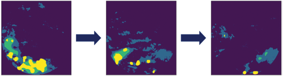
Figure 1: Scene 1
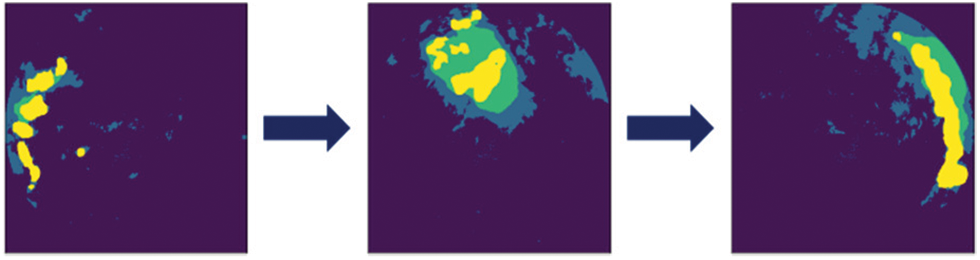
Figure 2: Scene 2
3.2 Improved Deep Convolutional Embedded Clustering
3.2.1 Convolutional AutoEncoder
The autoencoder is a trained neural network that can transform data into latent space non-linearly. When the dimension of this latent space is lower than that of the original space, the autoencoder reduces the dimension of the original data. With the popularity of convolutional neural networks, a new type of self-encoder has emerged, the convolutional autoencoder (CAE), which can achieve more efficient image feature representation and dimensionality reduction. CAE is composed of convolutional encoder and convolutional decoder, as shown in Fig. 3.
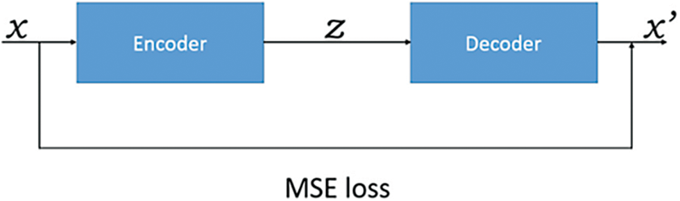
Figure 3: Structure of CAE
The convolutional encoder converts the input image (x) into a feature map (z) by Eq. (1), and the convolutional decoder converts the map (z) into an output image (x') by Eq. (2).
where w denotes the convolution kernel between x and z, w' denotes the convolution kernel between z and x', b and b' are deviations, and ReLU (Rectified Linear Units) is the activation function.
CAE generates a new code for each sample by minimizing the reconstruction error between the input and output of all samples, and its reconstruction loss function is defined as Eq. (3), where n denotes the number of input samples.
3.2.2 Deep Embedding Clustering
DEC [23] is a deep clustering algorithm which combines deep feature representation and image clustering. It uses a deep neural network to learn the mapping from the observation space to the low-dimensional latent space, and can obtain feature representation and clustering at the same time. DEC uses a denoising autoencoder for data preprocessing, then removes the decoder, defines the clustering loss function, and fine-tunes the retained encoder as shown in Eq. (4).
where KL divergence (Kullback-Leibler divergence) describes the difference between two probability distributions P and Q, P represents the true (target) distribution, and Q represents the fitted distribution of P.
Through the above steps, DEC completes the image clustering while completing the model parameter optimization. However, the fine-tuning step distorts the embedding space, resulting in a decrease in the representativeness of embedding features. An improved deep embedded clustering algorithm (IDEC) [24] is needed to solve the above problem by preserving the local structure of the data. The IDEC algorithm structure is shown in Fig. 4.
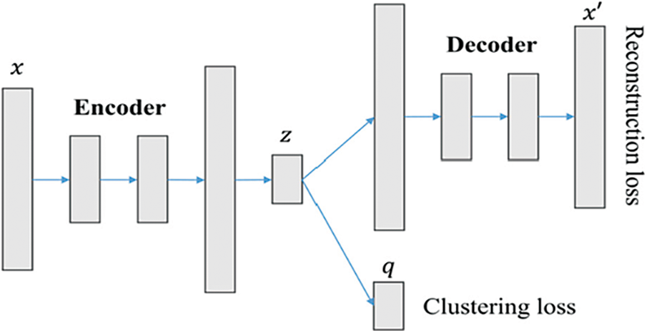
Figure 4: Structure of IDEC
IDEC uses an incomplete autoencoder to learn embedding features and preserve the local structure of the data generation distribution. After the pre-training, it is necessary to fine-tune the weighted sum of the reconstruction loss and the clustering loss to obtain a better clustering result while ensuring that the embedding space is not distorted to the utmost extent. IDEC uses both the clustering loss Lc defined in DEC and the reconstruction loss Lr defined in CAE to construct a new loss function, as shown in Eq. (7).
where λ is a hyperparameter that controls the degree of distortion of the embedding space. The larger the value of λ, the greater the impact of the clustering loss Lc on the overall objective function, and the easier to distort the embedding feature space. And when λ = 1 and Lr = 0, IDEC degenerates to DEC.
The deep convolution embedding clustering algorithm (DCEC) [25] replaces the full connection between the coding layer and the decoding layer of IDEC with a convolution operation, which is more conducive to extracting the hierarchical features of the images. The structure of DCEC is shown in Fig. 5, which is composed of CAE and clustering layers. DCEC uses three convolutional layers in the decoding layer and the coding layer, and then uses the flatten operation to flatten the feature vector, and finally obtains a 10-dimensional feature layer. The optimization goal of DCEC is the same as IDEC, and the joint optimization of reconstruction loss and clustering loss is still used, as Eq. (7).
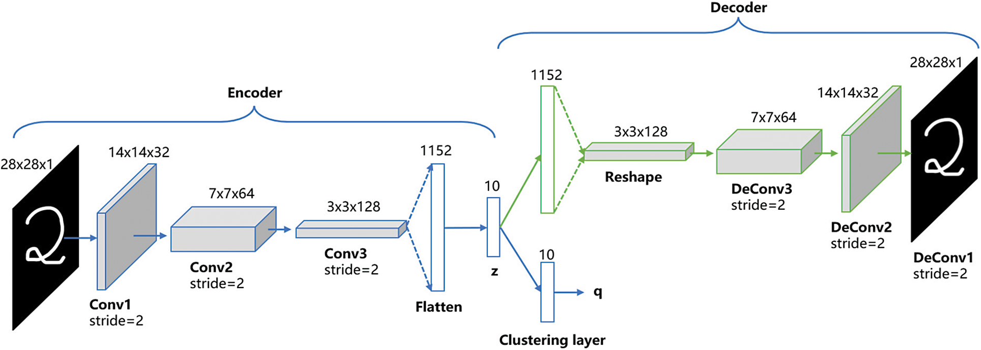
Figure 5: Structure of DCEC
It can be concluded that after the DCEC algorithm directly reduces the feature dimension to 10 dimensions after convolution and flatten operation, it may lead to the loss of a large number of image features. In order to solve this problem, we propose an improved deep convolutional embedding clustering, the optimization goal is the same as DCEC, and its structure is shown in Fig. 6.
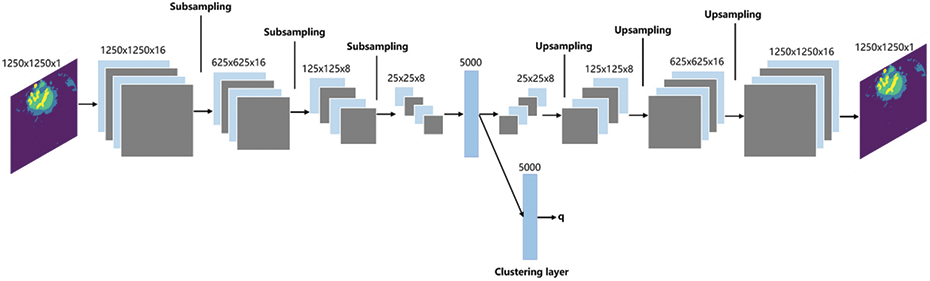
Figure 6: Structure of IDCEC
Compared with DCEC, IDCEC adds a padding operation to each of the convolutional layers in the coding layer and the decoding layer. Taking Fig. 6 as an example, 16 different convolution kernels are used to convolve the original weather images from 1250 × 1250 × 1 dimensions to 1250 × 1250 × 16 dimensions. This filling operation can ensure that the convolutional layer extracts more information from the previous layer. In addition, in order to ensure a certain degree of dimensionality reduction in the encoding process, we add a pooling layer after each convolutional layer, that is subsampling, which effectively reduces the image size. In Fig. 5, the DCEC can reduce the dimensionality of the image from 28 * 28 to 10, achieving the dimensionality reduction effect of 78.4 times, while the improved IDCEC model has achieved 1250 × 1250 dimensionality reduction to 5000, and the dimensionality reduction effect is 312.5 times.
It is easy to see that the time complexity of IDCEC consists of two main parts. 1) The time complexity of the CAE part is
The experiments use WAF data from the terminal area of Guangzhou Baiyun Airport in China for one year, including general meteorological conditions, systematic convective weather and thermal convective weather processes. The data also includes the east-west and north-south echoes. According to the impact degree on aircraft flights, the weather data is divided into four levels: none, mild, moderate and severe, corresponding to the four colors of purple, blue, green, and yellow in the images. The update frequency of the data is 10 minutes, the measurement accuracy is 200 m × 200 m and the size of the dataset is more than 10 thousand.
We use PCA+K-means (PCA-KM), histogram of oriented gradient+K-means (HOG-KM), and CAE+K-means (CAE-KM) as comparative methods to IDCEC. These methods have two stages: firstly, extracting the features of WAF images, and then clustering the features to obtain similar scenes. For IDCEC, since it is embedded clustering, the WAF image can be the direct input to the model to obtain the clusters of similar scenes.
4.2 Feature Extraction Experiment
We first use PCA to extract features from the WAF data. The change of the cumulative variance contribution rate of the principal components is shown in Fig. 7. We choose the corresponding principal components when the cumulative variance contribution rate is 90%, that is, the corresponding 200 principal components carry 90% of the information of the original data.
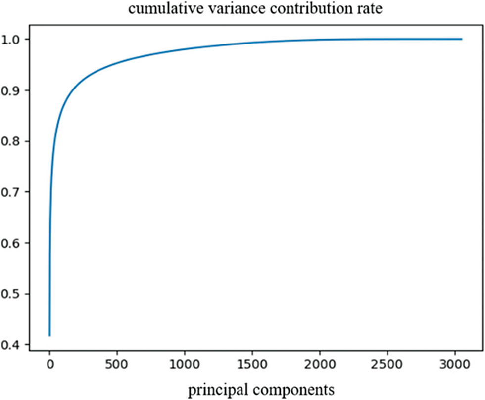
Figure 7: Cumulative variance contribution rate of PCA method
When we use histogram of oriented gradient (HOG) to reduce the dimensionality of WAF data, we extract 5000 HOG features to represent the original data. These 5000 features can effectively describe the edges of WAF images. Fig. 8 shows the horizontal and vertical gradient maps of a WAF image after HOG dimensionality reduction. It can be seen that the edge information of the image is well preserved.
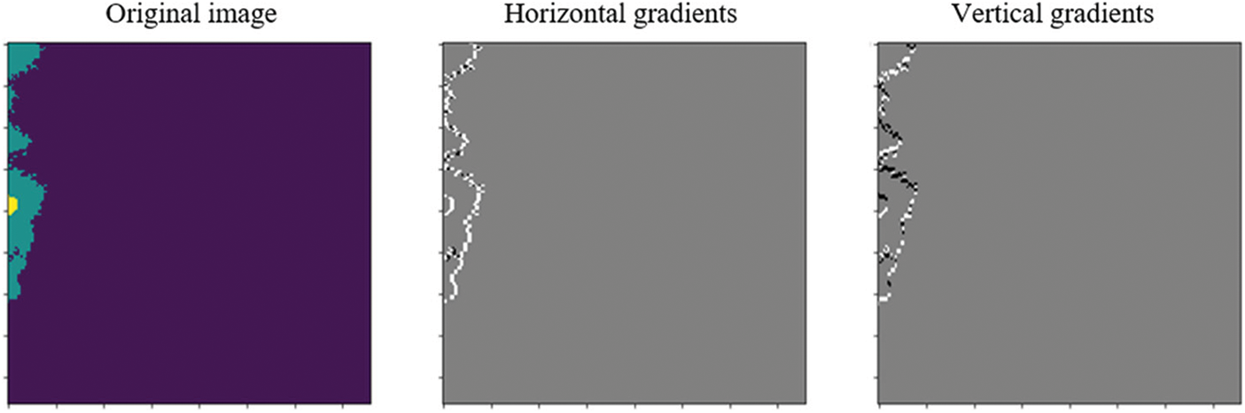
Figure 8: WAF image representation after HOG feature extraction
When we use CAE to reduce the dimensionality of the WAF image, the changes of the mean square errors on the training set and the validation set are shown in Fig. 9. The mean square errors on the two data sets decreased significantly with the growth of the training iterations, and the loss on the validation set finally stabilizes at about 0.01. This means that the data after dimensionality reduction with CAE can effectively retain the information of WAF images. We finally extract 5000 CAE features from the original WAF images.
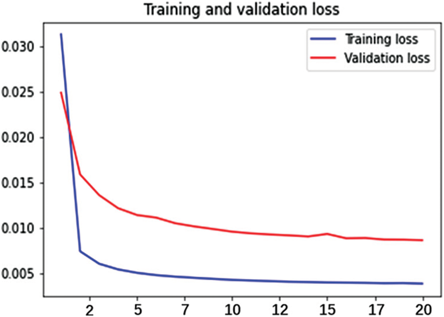
Figure 9: Changes of the loss on the training set and validation set
4.3 Training of the IDCEC Model
In order to train the IDCEC model proposed in Section 3.2, the cyclic iteration of IDEC is used to update the parameters of the coding layer, the decoding layer and the clustering loss layer. In order to verify the performance of the model, weather scenes are randomly divided into 3 categories, as shown in Epoch 0 in Fig. 10. As the number of training iterations increases, the distance between different weather scenes increases, which means that they have higher separability. At the same time, their spatial distribution is more reasonable, as shown in Epoch 10, Epoch 30 and Epoch 50 in Fig. 10. In the experiment, we selected the optimal parameter 0.1 of IDEC, and used the Adam optimizer and the learning rate setting used in reference [24] to complete the IDCEC model training on the deep learning framework TensorFlow.
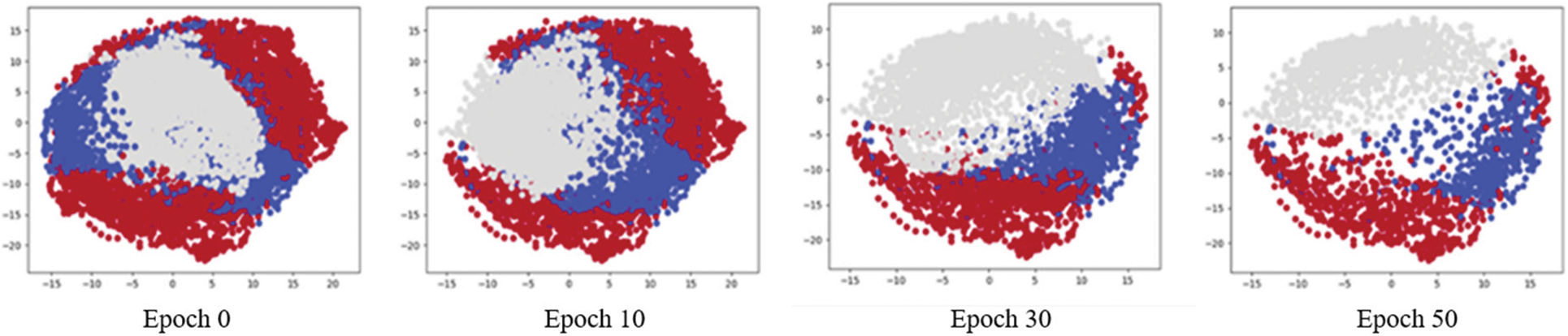
Figure 10: Training of IDCEC model
4.4.1 Comparison of Clustering Performance
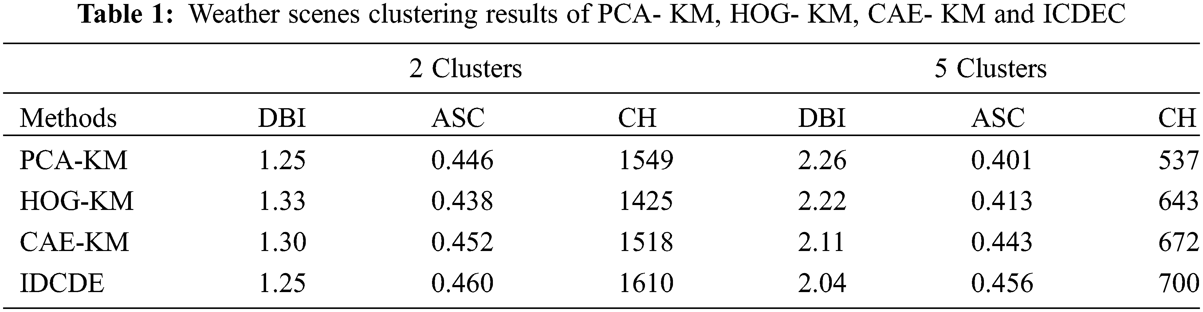
We use PCA-KM, HOG- KM, CAE- KM and ICDEC to cluster weather scenes into 2 and 5 clusters, and weather scenes in the same cluster can be regarded as similar scenes. We use the following three Davies-Bouldin Index (DBI), Average Silhouette Coefficient (ASC) and Calinski-Harabasz Score (CH) to evaluate the clustering performance of the four methods. The clustering results of the four methods are shown in Tab. 1. It can be seen that IDCEC obviously obtains the best clustering results.
4.4.2 Comparison of Visual Clustering Results
Fig. 11 shows the visualization results of the four methods for clustering scenes into 2 clusters. The first row of each sub-subgraph is a strong convective weather scene, and the second row is a weak/no convective weather scene. It can be seen that all the four methods can separate the strong convective weather from the weak/no convective weather. PCA-KM and IDCEC have better recognition results, while HOG-KM and CAE-KM divided some moderately strong convective weather scenes into weak/no convective weather scenes as shown in the second lines of Figs. 11b and 11c. This means that these two methods cannot accurately identify intermediate-level convective weather scenes.
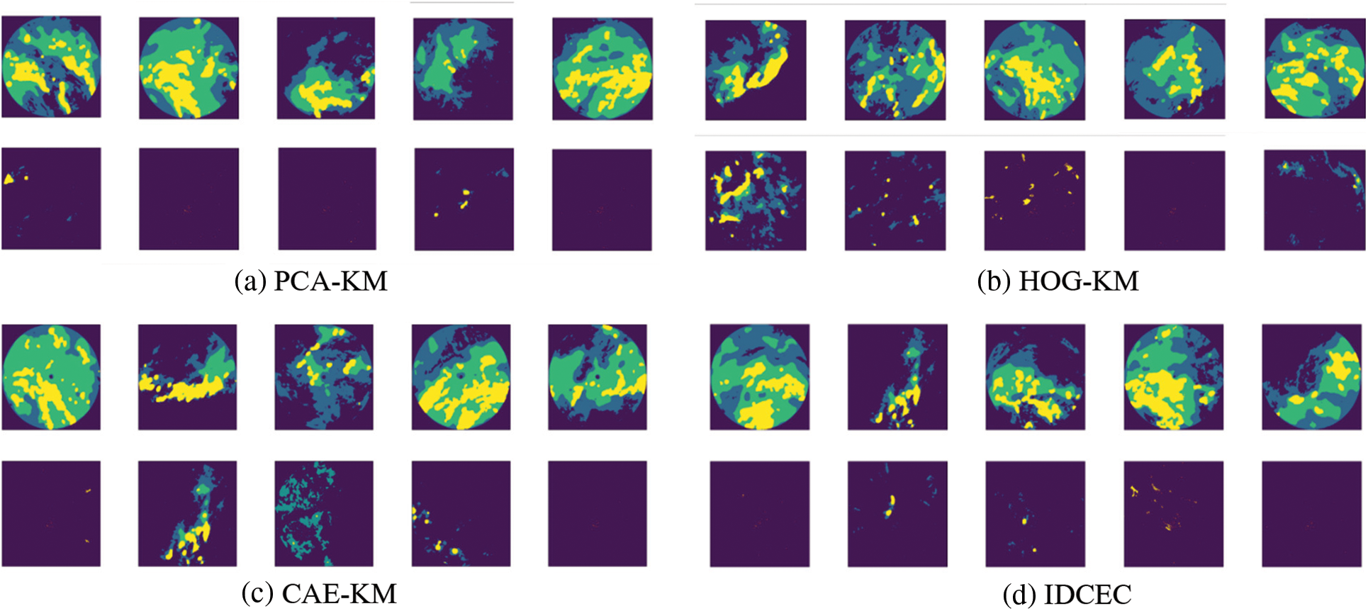
Figure 11: Similar weather scenes clustering results of 2 clusters
Fig. 12 respectively shows the visualization results of four methods for clustering the weather scenes into 5 clusters. The five rows in each figure represent five similar convective weather scenes.
Fig. 12a shows that the first scene corresponds to the situation with a little convective weather. The second scene corresponds to the situation with strong convective weather in the southeast of the airport and near the airport, but the algorithm fails to make a clear distinction between the two situations in space. The third scene and the fourth scene are both convective weather in the south of the airport, the former is less severe than the latter. The fifth scene describes the situation where most of the terminal area is covered by severe convective weather. It can be seen that PCA-KM can identify five types of similar scenes, but it cannot accurately reflect the distribution of convective weather.
Fig. 12b shows that among the five similar weather scenes clustered by HOG-KM, the first row is the scene with no/weak convective weather, the second row is the scene with convective weather near the airport, the third row is the scene with convective weather in the south of the airport, the fourth row is the scene with convective weather in the north of the airport, and the fifth row is the scene with convective weather covering a large area of the terminal area. It can be seen that this clustering result is better than the recognition result of PCA-KM and can better distinguish the distribution of convective weather. However, in the second row there are images with similar outlines to those in the third and fourth rows, which means that HOG-KM still has some difficulties in separating some scenes.
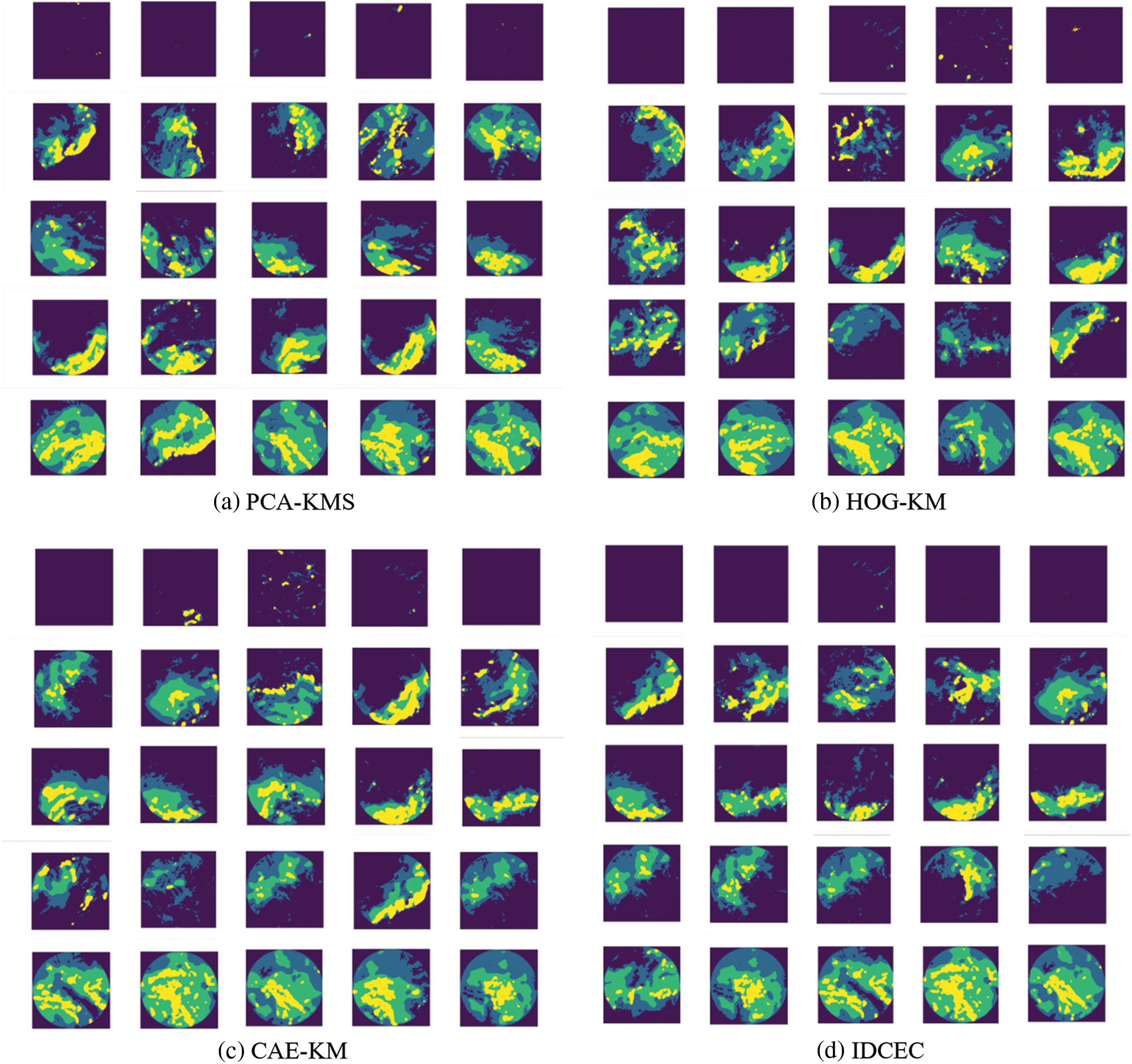
Figure 12: Similar weather scenes clustering results of 5 clusters
Fig. 12c shows that the convective weather distribution characteristics represented by the similar scene clustering results obtained by CAE-KM are similar to those of HOG-KM. The second line is a scene with a convective sky machine near the airport, but there is a convective weather in the south of the airport. The fourth line is a scene of convective weather in the north of the airport, but it shows that there is convective weather near the airport. It can be seen that, like HOG-KM, CAE-KM has some difficulties in accurately distinguishing some weather scenes.
Fig. 12d shows that IDCEC clearly identifies five convective weather scenes. The five scenes represented by the five rows from the first row to the bottom are: no/weak convective weather, convective weather near the airport, convective weather in the south of the airport, and convective weather in the northern of the airport and the terminal area cover a large area of convective weather. It can be concluded that the clustering result of IDCEC is better than the above three methods, especially for the second, third, and fourth scenes.
4.4.3 Analysis of Traffic Operation Characteristics under Different Weather Scenes
In this section, we correlated and analyzed the weather scenes clustered by IDCEC with the actual flow in the terminal area, trying to find the relationship between the two. We select the weather scene and actual flow in the terminal area during the busy period of 12:00–15:00 when the demand flow is relatively stable. The analysis results are shown in Figs. 13 and 14. Fig. 13 compares the flow distributions of the 2 clusters of similar weather scenes. The first cluster is the scene with convective weather, and the second one is the scene with no/weak convective weather. It can be seen that the flow level of the first cluster is significantly lower than that of the second one, which means that convective weather has a obvious impact on the flow. Fig. 14 compares the flow distributions of the 5 clusters of similar weather scenes. The first cluster has the highest flow distribution, and the fifth cluster has the lowest. The first cluster and the fifth cluster respectively correspond to the weak/no convective weather scene and the scene where most of the terminal area covers convective weather. The second cluster is a scene with convective weather near the airport, and its flow mode is 8 flights/10 min, which is only better than the fifth cluster. The third cluster and the fourth cluster correspond to the convective weather scene in the south of the airport and the convective weather scene in the north of the airport, respectively. It can be seen from the figure that the flow of the terminal area mainly occurs in the north, therefore, when the north of the airport is affected by convective weather, the flow will drop more.
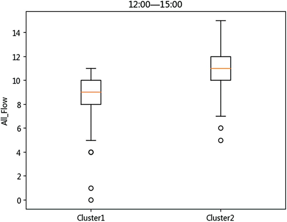
Figure 13: Flow distributions of 2 similar weather scenes clustered by IDCEC
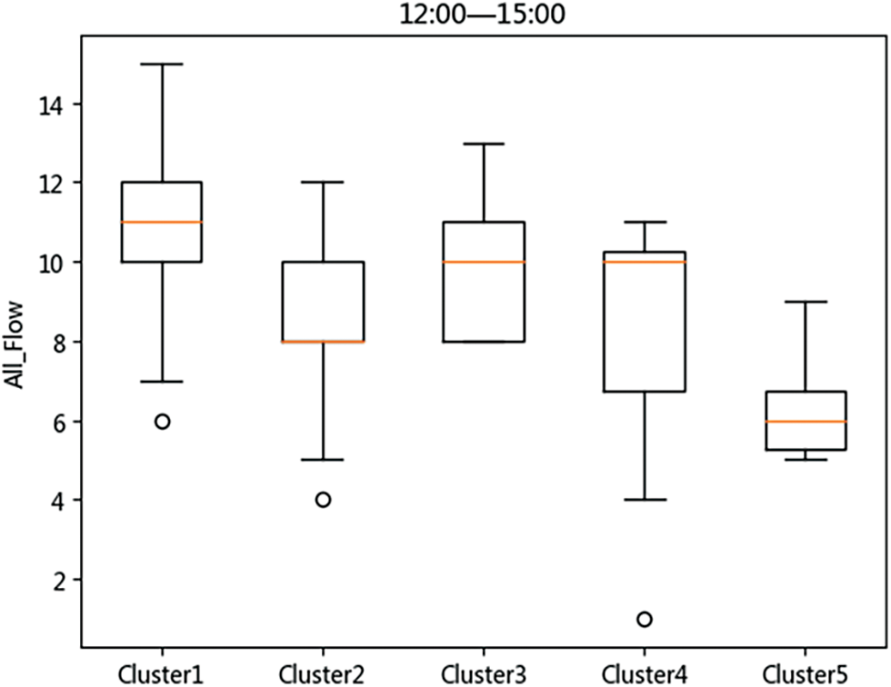
Figure 14: Flow distributions of 5 similar weather scenes clustered by IDCEC
From the analysis, we can conclude that IDCEC proposed in this paper can accurately identify similar weather scenes in the terminal area, and each scene is consistent with its actual flight flow distribution. There is a certain relationship pattern between the scene and the flight flow.
Therefore, based on the weather scene classification results of IDCEC, the differentiated traffic distribution under different scenes in the terminal area can be effectively analyzed and extracted. When the acquired weather forecast data is most similar to a certain type of scenes, then the historical traffic distribution features under that type of scenes can be used as an important reference for airspace capacity prediction, supporting the rapid quantitative prediction of the terminal area capacity level range and applying it to the actual traffic management decision, which is the starting point of this paper's research. This paper will serve as the research basis of airspace capacity evaluation techniques based on weather scene classification.
In order to classify similar weather scenes in the terminal area more accurately, this paper proposes an improved deep convolutional self-encoding embedded clustering method (IDCEC). By improving the encoding and decoding layers, IDCEC achieves a greater dimensionality reduction rate for weather images while retaining more information. We compared the proposed IDCEC method with the traditional PCA-KMS, HOG-KMS, and CAE-KMS on the historical weather images in the terminal area of Guangzhou Baiyun Airport. IDCEC has shown the best performance on both the clustering indexes and the visualization images of the clustering results. IDCEC can distinguish five types of similar weather scenes more accurately, namely, no/weak convection weather scenes, convective weather scenes near the airport, convective weather scenes in the south of the airport, convection weather scenes in the north of the airport, and convective weather scenes covering a large area of the terminal area. Furthermore, we analyzed the actual traffic flow in the airport terminal area under different weather scenes, and verified that there is a clear consistency between the two. This means the recognition of similar weather scenes can support traffic control decisions.
Funding Statement: This work was supported by the Fundamental Research Funds for the Central Universities under Grant NS2020045. Y.L.G received the grant.
Conflicts of Interest:The authors declare that they have no conflicts of interest to report regarding the present study.
1. A. V. Sadovsky and K. D. Bilimoria, “Risk-hedged approach for re-routing air traffic under weather uncertainty,” in 16th AIAA Aviation Technology, Integration, and Operations Conf., Washington D.C., pp. 3601, 2016. [Google Scholar]
2. O. Ohneiser, M. Kleinert, K. Muth, O. Gluchshenko and M. M. Temme, “Bad weather highlighting: advanced visualization of severe weather and support in air traffic control displays,” in 2019 IEEE/AIAA 38th Digital Avionics Systems Conf. (DASC), San Diego, California, IEEE, pp. 1–10, 2019. [Google Scholar]
3. M. A. Asencio, “Clustering approach for analysis of convective weather impacting the NAS,” in 2012 Integrated Communications, Navigation and Surveillance Conf., Herndon, Virginia, IEEE, pp. N4-1, 2012. [Google Scholar]
4. K. Kuhn, A. Shah and C. Skeels, “Characterizing and classifying historical days based on weather and air traffic,” in 2015 IEEE/AIAA 34th Digital Avionics Systems Conf. (DASC), Prague, Czech Republic, IEEE, pp. 1C3-1, 2015. [Google Scholar]
5. X. R. Zhang, W. F. Zhang, W. Sun, X. M. Sun and S. K. Jha, “A robust 3-D medical watermarking based on wavelet transform for data protection,” Computer Systems Science and Engineering, vol. 41, no. 3, pp. 1043–1056, 2022. [Google Scholar]
6. X. R. Zhang, X. Sun, X. M. Sun, W. Sun and S. K. Jha, “Robust reversible audio watermarking scheme for telemedicine and privacy protection,” CMC-Computers, Materials & Continua, vol. 71, no. 2, pp. 3035–3050, 2022. [Google Scholar]
7. K. D. Kuhn, “A methodology for identifying similar days in air traffic flow management initiative planning,” Transportation Research Part C: Emerging Technologies, vol. 69, pp. 1–15, 2016. [Google Scholar]
8. R. Delaura, M. Robinson, R. Todd and K. Mackenzie, “Evaluation of weather impact models in departure management decision support: Operational performance of the Route Availability Planning Tool (RAPT) prototype,” Weather and Forecasting, vol. 21, pp. 220–310, 2012. [Google Scholar]
9. W. D. Love, W. C. Arthur, W. S. Heagy and D. Kirk, “Assessment of prediction error impact on resolutions for aircraft and severe weather avoidance,” in AIAA 4th Technology, Integration, and Operations Forum, Chicago, Illinois, pp. 1–10, 2004. [Google Scholar]
10. R. Delaura and S. Allan, “Route selection decision support in convective weather: A case study of the effects of weather,” in 5th EuroControl/FAA ATM R&D Seminar, Budapest, Hungary, 2003. [Google Scholar]
11. B. Hoffman, J. Krozel and R. Jakobovits, “Weather forecast requirements to facilitate fix-based airport ground delay programs,” in 86th AMS Annual Meeting, Atlanta, pp. 1–6, 2006. [Google Scholar]
12. J. Krozel, J. S. B. Mitchell, Polishchuk and J. Prete, “Capacity estimation for airspaces with convective weather constraints,” in AIAA Guidance, Navigation and Control Conf. and Exhibit, Hilton head, South Carolina, pp. 1–15, 2007. [Google Scholar]
13. J. Prete and J. Krozel, “Benefit of a raycast weather severity metric for estimating transition airspace capacity,” in 10th AIAA Aviation Technology, Integration, and Operations Conf., Fort Worth, Texas, pp. 1–12, 2010. [Google Scholar]
14. S. Grabbe, B. Sridhar and A. Mukherjee, “Clustering days and hours with similar airport traffic and weather conditions,” Journal of Aerospace Information Systems, vol. 11, no. 11, pp. 751–763, 2014. [Google Scholar]
15. J. Gu, Z. Wang, J. Kuen, M. Lianyang and W. Gang, “Recent advances in convolutional neural networks,” Pattern Recognition, vol. 77, no. 11, pp. 354–377, 2018. [Google Scholar]
16. R. Dubey and J. Agrawal, “An improved genetic algorithm for automated convolutional neural network design,” Intelligent Automation and Soft Computing, vol. 32, no. 2, pp. 747–763, 2022. [Google Scholar]
17. R. Chen, L. Pan, Y. Zhou and Q. Lei, “Image retrieval based on deep feature extraction and reduction with improved cnn and pca,” Journal of Information Hiding and Privacy Protection, vol. 2, no. 2, pp. 67–76, 2020. [Google Scholar]
18. G. E. Hinton and R. R. Salakhutdinov, “Reducing the dimensionality of data with neural networks,” Science, vol. 313, no. 5786, pp. 504–507, 2006. [Google Scholar]
19. J. Masci, U. Meier, D. Cireşan and J. Schmidhuber, “Stacked convolutional auto-encoders for hierarchical feature extraction,” in Int. Conf. on Artificial Neural Networks, Berlin, Heidelberg, Springer, pp. 52–59, 2011. [Google Scholar]
20. A. Romero, C. Gatta and G. Camps-Valls, “Unsupervised deep feature extraction for remote sensing image classification,” IEEE Transactions on Geoscience and Remote Sensing, vol. 54, no. 3, pp. 1349–1362, 2015. [Google Scholar]
21. Y. Zhang, K. Lee and H. Lee, “Augmenting supervised neural networks with unsupervised objectives for large-scale image classification,” in Int. Conf. on Machine Learning, New York City, United States, pp. 612–621, 2016. [Google Scholar]
22. W. Fang, L. Pang and W. N. Yi, “Survey on the application of deep reinforcement learning in image processing,” Journal on Artificial Intelligence, vol. 2, no. 1, pp. 39–58, 2020. [Google Scholar]
23. P. Ji, T. Zhang, H. Li, M. Salzmann and I. Reid, “Deep subspace clustering networks,” in Advances in Neural Information Processing Systems, Long Beach, CA, USA, pp. 24–33, 2017. [Google Scholar]
24. X. Guo, L. Gao, X. Liu and J. Yin, “Improved deep embedded clustering with local structure preservation,” in IJCAI, Melbourne, Australia, pp. 1753–1759, 2017. [Google Scholar]
25. X. Guo, X. Liu, E. Zhu and J. Yin, “Deep clustering with convolutional autoencoders,” in Int. conf. on neural information processing, Cham, Springer, pp. 373–382, 2017. [Google Scholar]
 | This work is licensed under a Creative Commons Attribution 4.0 International License, which permits unrestricted use, distribution, and reproduction in any medium, provided the original work is properly cited. |